Choosing the Energy Sources Needed for Utilities in the Design and Refurbishment of Buildings


Abstract
:1. Introduction
2. The Mathematical Model that Was Used
- C0 represents the initial investment costs (EUR);
- CE is the annual cost of energy that is consumed at the reference year level (EUR/year);
- CM is the annual operating and maintenance (O&M) cost (EUR/year);
- CCO2 is the annual cost of carbon dioxide emissions (EUR/year);
- f is the annual rate of increase in the cost of energy;
- i is the discount rate;
- k is index corresponding to the energy source that is used;
- N is the calculation period.
- α, β, …, ω are the different energy carriers;
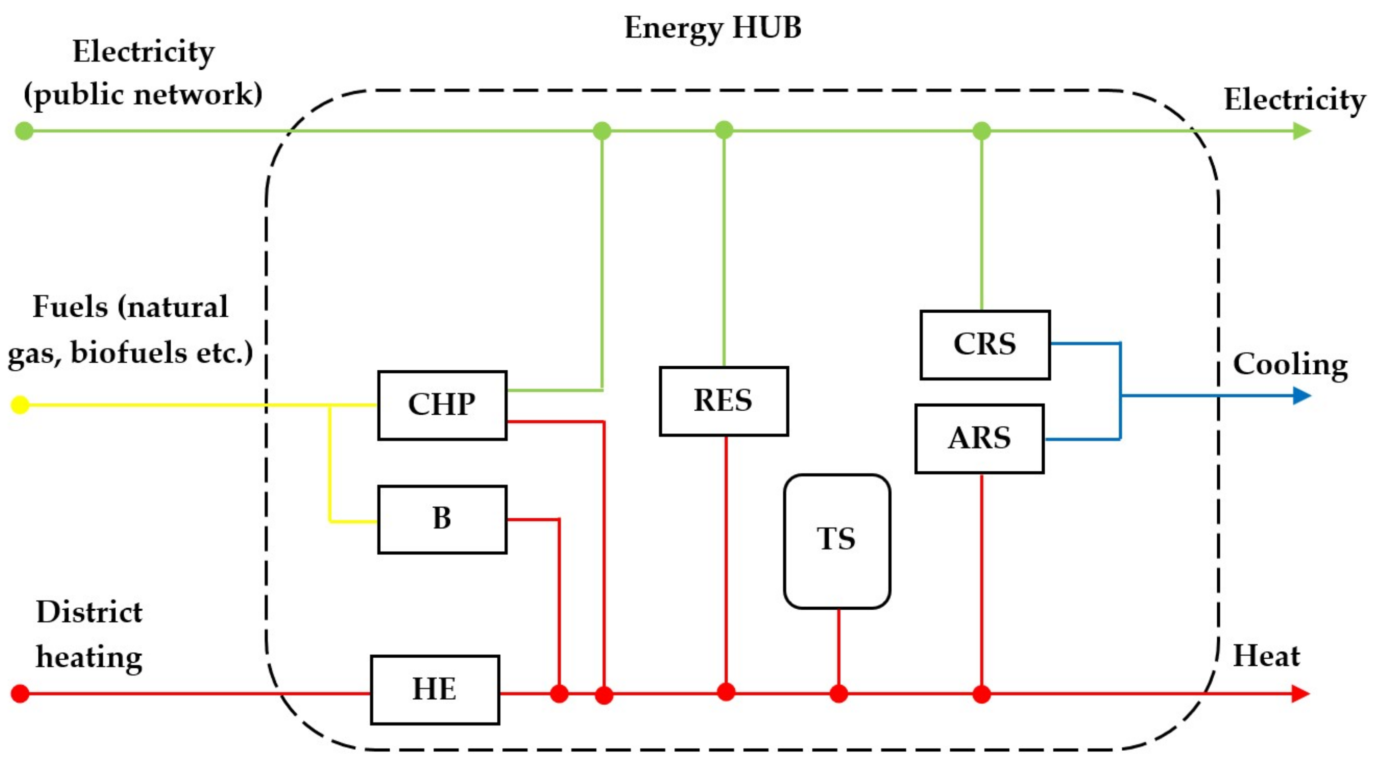
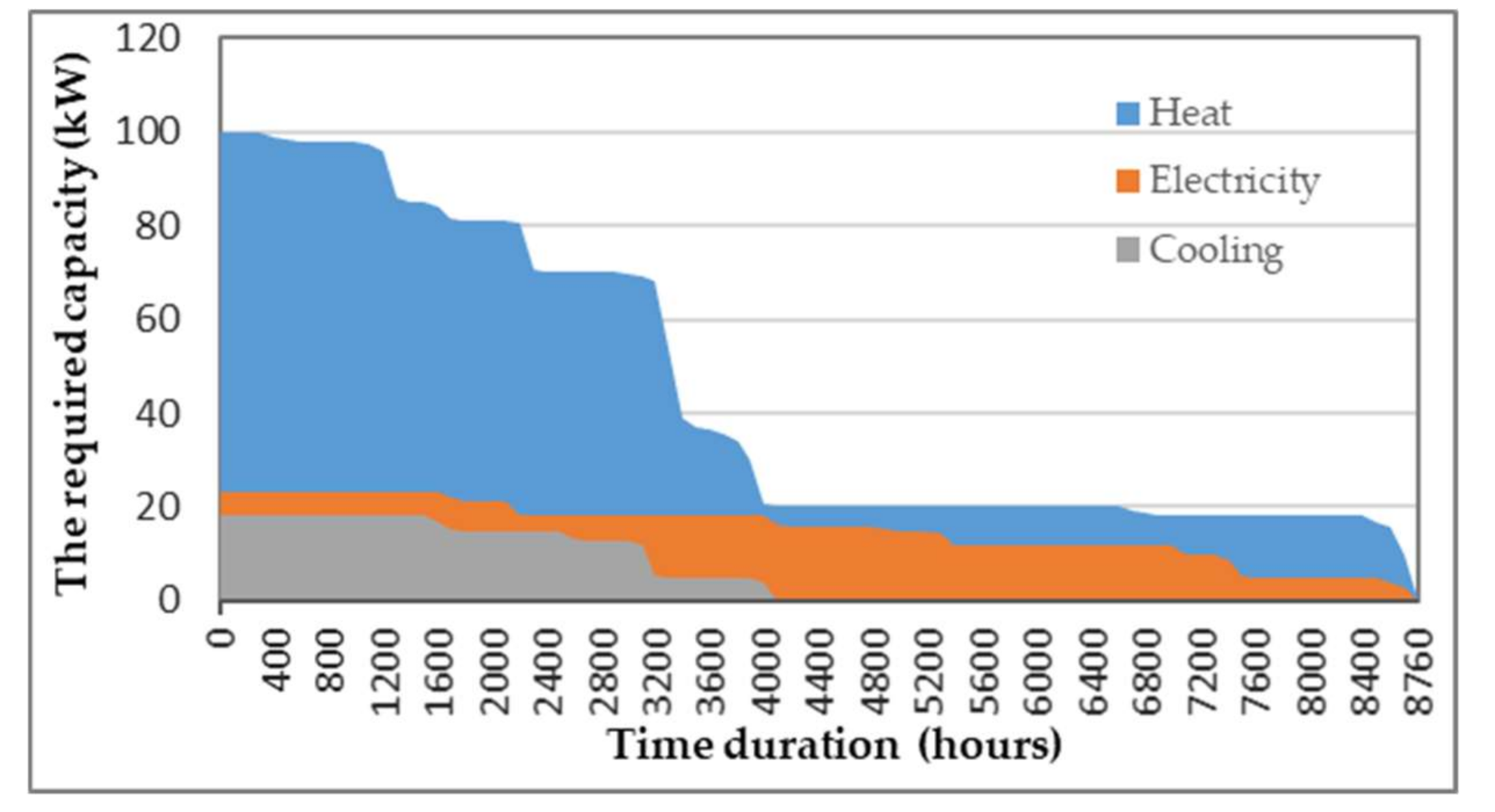
- L is the load matrix (the energy consumption of the building);
- P is the power matrix of the energy carriers that enter the hub;
- C is the converter coupling matrix.
3. Example Application
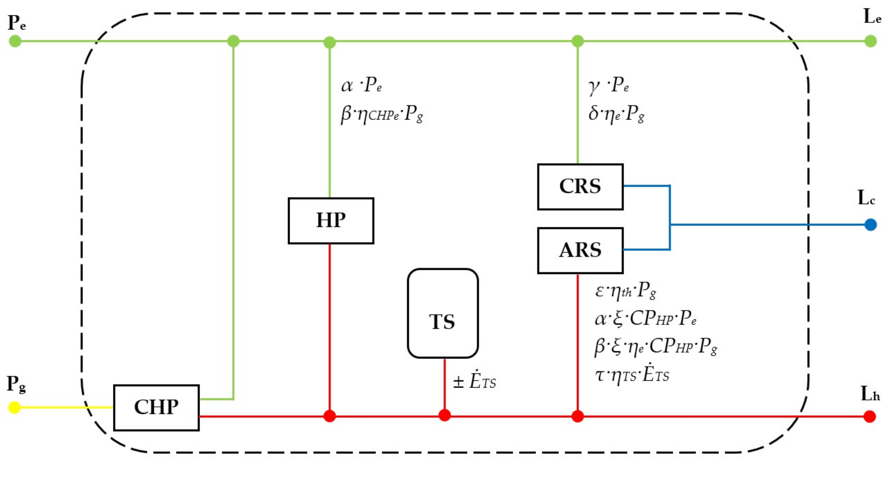
- Scenario 1 (Figure 4) includes the following energy sources: the electricity supply from the public network; two combined heat and power plants (CHPs) on natural gas fuel; a heat pump; a heat storage system; a compression refrigeration system; and an absorption refrigeration system.
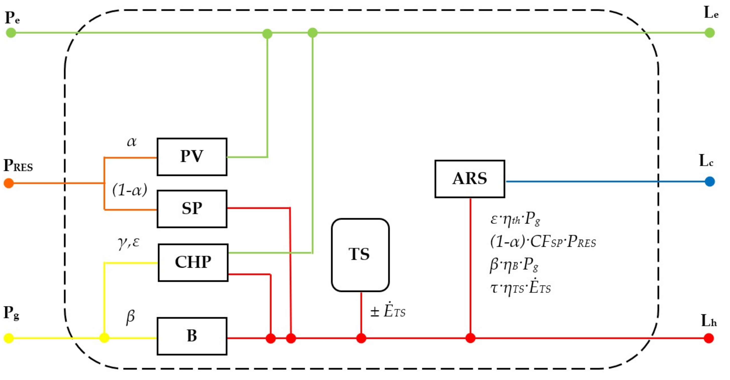
- Scenario 2 (Figure 5) includes the following energy sources: the electricity supply from the public network; a combined heat and power plant (CHP) on natural gas fuel; a natural gas boiler (as a peak source); a system of photovoltaic panels; a system of solar thermal panels; a heat storage system; and an absorption refrigeration system.
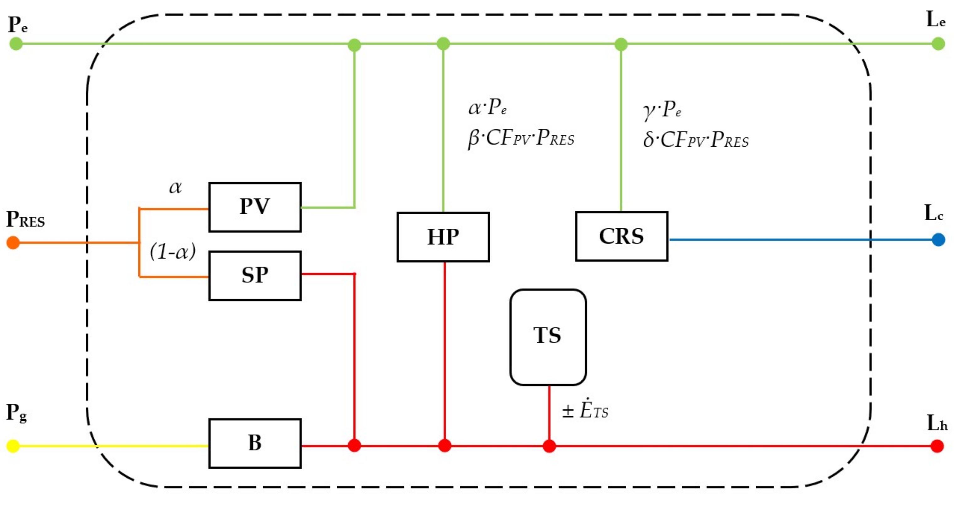
- Scenario 3 (Figure 6) includes the following energy sources: the electricity supply from the public network; a heat pump; a natural gas boiler (as a peak source); a system of photovoltaic panels; a system of solar thermal panels; a heat storage system; and a compression refrigeration system.
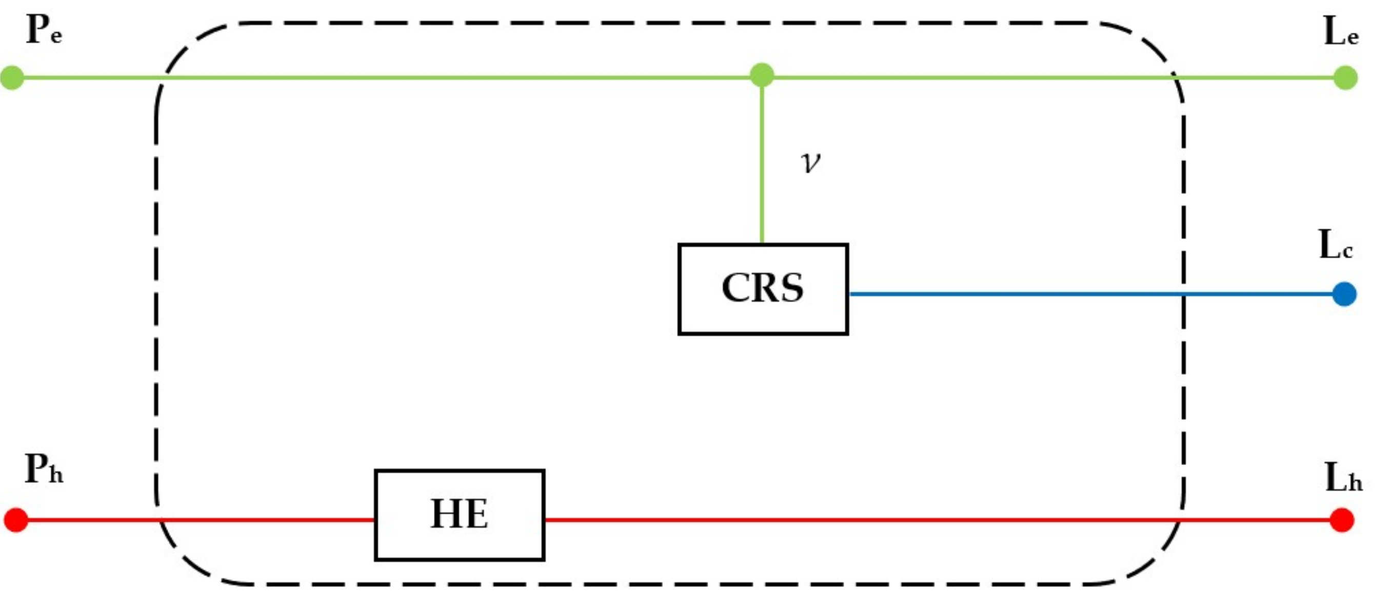
- Scenario 4 (Figure 7) includes the following energy sources: the electricity supply from the public network; the heat supply from the district heating system and a compression refrigeration system.
- α is the share of electricity to supply the heat pump;
- β is the share of natural gas that is converted into electricity to supply the heat pump;
- γ is the share of electricity to supply the compression refrigeration system;
- δ is the share of natural gas that is converted into electricity for the compression refrigeration system;
- ε is the share of natural gas that is converted into heat for the absorption refrigeration system;
- ξ is the share of heat from the heat pump for the absorption refrigeration system;
- τ is the share of heat that is stored to supply the absorption refrigeration system.
- ηe is the efficiency of electricity generation in cogeneration;
- ηthis the efficiency of heat generation in cogeneration;
- CPHP is the coefficient of the performance of the heat pump;
- CPCR is the coefficient of the performance of the compression refrigeration system;
- CPAR is the coefficient of the performance of the absorption refrigeration system;
- eTS is the storage efficiency of thermal energy—Equation (8).
- α is the share of electricity from renewable energy sources;
- β is the share of heat from the boiler to supply the absorption refrigeration system;
- γ is the share of gas that is converted into electricity in CHP;
- ε is the share of gas that is converted into heat in CHP for the absorption refrigeration system;
- τ is the share of heat that is stored.
- ηe is the efficiency of electricity generation in cogeneration;
- ηth is the efficiency of heat generation in cogeneration;
- CFPV is the nominal capacity utilization factor for the photovoltaic panels;
- CFSP is the nominal capacity utilization factor for the solar thermal panels;
- CPAR is the coefficient of the performance of the absorption refrigeration system;
- ηB is the boiler efficiency;
- eTS is the storage efficiency of thermal energy—Equation (8).
- α is the share of electricity from renewable energy sources;
- β is the share of electricity from the photovoltaic panels to supply the heat pump;
- γ is the share of electricity from the public network for the compression refrigeration system;
- δ is the share of electricity from the photovoltaic panels for the compression refrigeration system;
- τ is the share of heat that is stored to supply the absorption refrigeration system.
- CPHP is the coefficient of the performance of the heat pump;
- CPCR is the coefficient of the performance of the compression refrigeration system;
- CFPV is the nominal capacity utilization factor for the photovoltaic panels;
- CFSP is the nominal capacity utilization factor for the solar thermal panels;
- ηB is the boiler efficiency;
- eTS is the storage efficiency of thermal energy—Equation (8).
- CPCR is the coefficient of the performance of the compression refrigeration system;
- ηHE is the efficiency of the heat exchanger.
4. Conclusions
Author Contributions
Conflicts of Interest
References
- Directive 2010/31/EU of the European Parliament and of the Council of 19 May 2010 the Energy Performance of Buildings. Available online: https://eur-lex.europa.eu/legal-content/EN/TXT/?uri=celex%3A32010L0031 (accessed on 10 February 2018).
- Directive 2009/28/EC of the European Parliament and of the Council of 23 April 2009 on the Promotion of the Use of Energy from Renewable Sources. Available online: https://eur-lex.europa.eu/legal-content/EN/ALL/?uri=celex%3A32009L0028 (accessed on 10 February 2018).
- Directive 2012/27/EU of the European Parliament and of the Council of 25 October 2012 on Energy Efficiency. Available online: https://eur-lex.europa.eu/legal-content/EN/TXT/?uri=celex:32012L0027 (accessed on 10 February 2018).
- Commission Recommendation (EU) 2016/1318 of 29 July 2016 on Guidelines for the Promotion of Nearly Zero-Energy Buildings and Best Practices to Ensure That, by 2020, All New Buildings Are Nearly Zero-Energy Buildings. Available online: https://eur-lex.europa.eu/legal-content/EN/TXT/?uri=CELEX%3A32016H1318 (accessed on 10 February 2018).
- Paoletti, G.; Pascuas, R.P.; Pernetti, R.; Lollini, R. Nearly Zero Energy Buildings: An Overview of the Main Construction Features across Europe. Buildings 2017, 7, 43. [Google Scholar] [CrossRef]
- Péan, T.Q.; Ortiz, J.; Salom, J. Impact of Demand-Side Management on Thermal Comfort and Energy Costs in a Residential nZEB. Buildings 2017, 7, 37. [Google Scholar] [CrossRef]
- Cornaro, C.; Basciano, G.; Puggioni, V.A.; Pierro, M. Energy Saving Assessment of Semi-Transparent Photovoltaic Modules Integrated into NZEB. Buildings 2017, 7, 9. [Google Scholar] [CrossRef]
- Moghimi, S.M.; Sarlak, G. Energy Management Optimizing in Multi Carrier Energy Systems Considering Net Zero Emission and CHP Temperature Effects. Phys. Sci. Int. J. 2016, 10, 1–11. [Google Scholar] [CrossRef]
- Touloupaki, E.; Theodosiou, T. Optimization of External Envelope Insulation Thickness: A Parametric Study. Energies 2017, 10, 270. [Google Scholar] [CrossRef]
- González, A.G.; Bouillard, P.; Román, C.A.A.; Trachte, S.; Evrard, A. TCS Matrix: Evaluation of optimal energy retrofitting strategies. Energy Procedia 2015, 83, 101–110. [Google Scholar] [CrossRef]
- Konstantinou, T.; Knaack, U. Refurbishment of residential buildings: A design approach to energy-efficiency upgrades. Procedia Eng. 2011, 21, 666–675. [Google Scholar] [CrossRef]
- Congedo, P.M.; D’Agostino, D.; Baglivo, C.; Tornese, G.; Zacà, I. Efficient Solutions and Cost-Optimal Analysis for Existing School Buildings. Energies 2016, 9, 851. [Google Scholar] [CrossRef]
- Sheikhi, A.; Bahrami, S.; Ranjbar, A.M.; Sattari, S.; Adami, M. Financial Analysis for a Multi-Carrier Energy System Equipped with CCHP. In Proceedings of the International Conference on Renewable Energies and Power Quality (ICREPQ’13), Bilbao, Spain, 20–22 March 2013. [Google Scholar] [CrossRef]
- De Ruggiero, M.; Forestiero, G.; Manganelli, B.; Salvo, F. Buildings Energy Performance in a Market Comparison Approach. Buildings 2017, 7, 16. [Google Scholar] [CrossRef]
- Huo, D.; Le Blond, S.; Gu, C.; Wei, W.; Yu, D. Optimal operation of interconnected energy hubs by using decomposed hybrid particle swarm and interior-point approach. Electr. Power Energy Syst. 2018, 95, 36–46. [Google Scholar] [CrossRef]
- Glasgo, B.; Hendrickson, C.; Azevedo, I.L. Assessing the value of information in residential building simulation: Comparing simulated and actual building loads at the circuit level. Appl. Energy 2017, 203, 348–363. [Google Scholar] [CrossRef]
- Ha, T.; Zhang, Y.; Thang, V.V.; Huang, J. Energy hub modeling to minimize residential energy costs considering solar energy and BESS. J. Mod. Power Syst. Clean Energy 2017, 5, 389–399. [Google Scholar] [CrossRef]
- Mohammadi, M.; Noorollahi, Y.; Mohammadi-Ivatloo, B.; Yousefi, H.; Jalilnasbady, A.S. Optimal Scheduling of Energy Hubs in the Presence of Uncertainty—A Review. J. Energy Manag. Technol. 2017, 1, 1–17. [Google Scholar] [CrossRef]
- Prieto, A.; Knaack, U.; Auer, T.; Klein, T. Solar coolfacades: Framework for the integration of solar cooling technologies in the building envelope. Energy 2017, 137, 353–368. [Google Scholar] [CrossRef]
- Abdullah, H.K.; Alibaba, H.Z. Retrofits for Energy Efficient Office Buildings: Integration of Optimized Photovoltaics in the Form of Responsive Shading Devices. Sustainability 2017, 9, 2096. [Google Scholar] [CrossRef]
- Pavicevic, M.; Novosel, T.; Puksec, T.; Duic, N. Hourly optimization and sizing of district heating systems considering building refurbishment e Case study for the city of Zagreb. Energy 2017, 137, 1264–1267. [Google Scholar] [CrossRef]
- Bahrami, S.; Safe, F. A Financial Approach to Evaluate an Optimized Combined Cooling, Heat and Power System. Energy Power Eng. 2017, 5, 352–362. [Google Scholar] [CrossRef]
- Nižetić, S.; Papadopoulos, A.M.; Tinac, G.M.; Rosa-Clot, M. Hybrid energy scenarios for residential applications based on the heat pump split air-conditioning units for operation in the Mediterranean climate conditions. Energy Build. 2017, 140, 110–120. [Google Scholar] [CrossRef]
- Li, C.; Ding, Z.; Zhao, D.; Yi, J.; Zhang, G. Building Energy Consumption Prediction: An Extreme Deep Learning Approach. Energies 2017, 10, 1525. [Google Scholar] [CrossRef]
- Burman, E.; Mumovic, D.; Kimpian, J. Towards measurement and verification of energy performance under the framework of the European directive for energy performance of buildings. Energy 2014, 77, 153–163. [Google Scholar] [CrossRef]
- Ko, W.; Park, J.K.; Kim, M.K.; Heo, J.H. A Multi-Energy System Expansion Planning Method Using a Linearized Load-Energy Curve: A Case Study in South Korea. Energies 2017, 10, 1663. [Google Scholar] [CrossRef]
- Geidl, M. Integrated Modeling and Optimization of Multi-Carrier Energy Systems. PhD Thesis, Power Systems Laboratory, ETH Zurich, Zurich, Switzerland, 2007. [Google Scholar]
- Geidl, M.; Andersson, G. Operational and Structural Optimization of Multi-Carrier Energy Systems. Eur. Trans. Electr. Power 2006, 16, 1–16. [Google Scholar] [CrossRef]
- Simader, G.R.; Krawinkler, R.; Trnka, G. Micro CHP Systems: State-of-the-Art; Austrian Energy Agency: Vienna, Austria, March 2006; Available online: https://ec.europa.eu/energy/intelligent/projects/sites/iee-projects/files/projects/documents/green_lodges_micro_chp_state_of_the_art.pdf (accessed on 11 February 2018).
- Fleiter, T.; Steinbach, J.; Ragwitz, M. Mapping and Analyses of the Current and Future (2020–2030) Heating/Cooling Fuel Deployment (Fossil/Renewables). Fraunhofer ISI, Final Report. March 2016. Available online: https://ec.europa.eu/energy/sites/ener/files/documents/Report%20WP2.pdf (accessed on 11 February 2018).
- Hauer, A. Thermal Energy Storage. IEA-ETSAP and the International Renewable Energy Agency (IRENA), January 2013. Available online: https://www.irena.org/DocumentDownloads/Publications/IRENA-ETSAP%20Tech%20Brief%20E17%20Thermal%20Energy%20Storage.pdf (accessed on 11 February 2018).
- Energy Prices and Costs in Europe. Available online: https://ec.europa.eu/energy/en/data-analysis/market-analysis (accessed on 10 February 2018).
- Commission Delegated Regulation (EU) No 244/2012 of 16 January 2012 Supplementing Directive 2010/31/EU of the European Parliament and of the Council on the Energy Performance of Buildings by Establishing a Comparative Methodology Framework for Calculating Cost-Optimal Levels of Minimum Energy Performance Requirements for Buildings and Building Elements. Available online: http://eur-lex.europa.eu/eli/reg_del/2012/244/oj (accessed on 10 February 2018).


| Type of Technology | Nominal Power/Energy | Specific Investment | O&M costs (% of Investment/Year) | Conversion Efficiency |
| CHP | 18 kWe36 kWth | 1500 EUR/kWe | 5.0% | ηe = 30%ηth = 55% |
| HP | 65 kW (heat) | 1200 EUR/kW | 3.2% | CPHP = 4 |
| TS | 200 kWh | 20 EUR/kWh | 2.0% | ηTS = 90% |
| CRS | 18 kW (cool) | 110 EUR/kW | 1.2% | CPCR = 3 |
| ARS | 18 kW (cool) | 600 EUR/kW | 2.5% | CPAR = 0.75 |
| Type of Technology | Nominal Power/Energy | Specific Investment | O&M costs (% of Investment/Year) | Conversion Efficiency |
|---|---|---|---|---|
| CHP | 18 kWe36 kWth | 1500 EUR/kWe | 5.0% | ηe = 30%ηth = 55% |
| B | 75 kWth | 127 EUR/kWth | 2.5% | ηB = 94% |
| PV | 15 kW | 2500 EUR/kW | 1.0% | CFPV = 16% |
| SP | 60 kW | 300 EUR/kW | 1.0% | CFSP = 16% |
| TS | 200 kWh | 20 EUR/kWh | 2.0% | ηTS = 90% |
| ARS | 18 kW (cool) | 600 EUR/kW | 2.5% | CPAR = 0.75 |
| Type of Technology | Nominal Power/Energy | Specific Investment | O&M costs (% of Investment/Year) | Conversion Efficiency |
|---|---|---|---|---|
| HP | 65 kW (heat) | 1200 EUR/kW | 3.2% | CPHP = 4 |
| B | 75 kWth | 127 EUR/kW | 2.5% | ηB = 94% |
| PV | 15 kW | 2500 EUR/kW | 1.0% | CFPV = 16% |
| SP | 60 kW | 300 EUR/kW | 1.0% | CFSP = 16% |
| TS | 200 kWh | 10 EUR/kWh | 2.0% | ηTS = 90% |
| CRS | 18 kW (cool) | 110 EUR/kW | 1.2% | CPCR = 3 |
| Type of Technology | Nominal Power/Energy | Specific Investment | O&M costs (% of Investment/Year) | Conversion Efficiency |
|---|---|---|---|---|
| HE | 100 kW (heat) | 10 EUR/kW | 1.0% | ηHE = 98% |
| CRS | 18 kW (cool) | 110 EUR/kW | 1.2% | CPCR = 3 |
| Electricity (EUR/kW) | Natural Gas (EUR/kW) | Heat (EUR/kW) |
|---|---|---|
| 0.105 | 0.027 | 0.045 |
| Structure of the Cost | Scenario 1 | Scenario 2 | Scenario 3 | Scenario 4 |
|---|---|---|---|---|
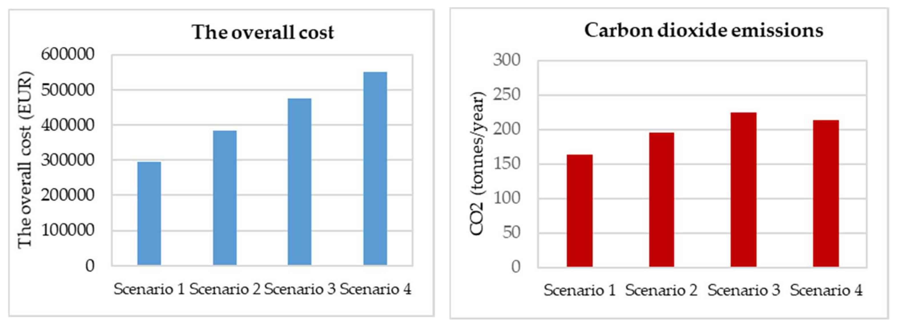
| The overall costs (EUR) | 295,188 | 399,217 | 478,707 | 549,425 |
| of which: | ||||
| The investment costs | 41.26% | 38.76% | 43.34% | 2.28% |
| The cost of energy consumed | 37.93% | 42.28% | 39.72% | 87.55% |
| The operating and maintenance costs | 7.55% | 6.77% | 5.54% | 0.41% |
| The cost of carbon dioxide emissions | 13.26% | 12.19% | 11.39% | 9.76% |
© 2018 by the authors. Licensee MDPI, Basel, Switzerland. This article is an open access article distributed under the terms and conditions of the Creative Commons Attribution (CC BY) license (http://creativecommons.org/licenses/by/4.0/).
Share and Cite
Atănăsoae, P.; Pentiuc, R.D. Choosing the Energy Sources Needed for Utilities in the Design and Refurbishment of Buildings. Buildings 2018, 8, 54. https://doi.org/10.3390/buildings8040054
Atănăsoae P, Pentiuc RD. Choosing the Energy Sources Needed for Utilities in the Design and Refurbishment of Buildings. Buildings. 2018; 8(4):54. https://doi.org/10.3390/buildings8040054
Chicago/Turabian StyleAtănăsoae, Pavel, and Radu Dumitru Pentiuc. 2018. "Choosing the Energy Sources Needed for Utilities in the Design and Refurbishment of Buildings" Buildings 8, no. 4: 54. https://doi.org/10.3390/buildings8040054
APA StyleAtănăsoae, P., & Pentiuc, R. D. (2018). Choosing the Energy Sources Needed for Utilities in the Design and Refurbishment of Buildings. Buildings, 8(4), 54. https://doi.org/10.3390/buildings8040054