Abstract
The construction of a new facility in an urban area, such as a downtown area, involves considerable earthwork excavation most of the time. Measuring the actual productivity of earthwork operations that involve heavy machinery can be a complex task for project managers. The complexity contributes to the impact of the many factors involved, the required accuracy, and the uncertainties associated with such operations. Traditionally, measuring actual productivity is carried out manually by measuring the actual quantities of the excavated earth. Measuring actual productivity manually is time-consuming and not necessarily accurate. The paper presents a case study project in Montreal to investigate the application of a developed methodology that is affordable for small to medium size contractors. It integrates the GPS and fuzzy set theory as an alternate effective methodology for measuring actual onsite productivity during the construction stage in an urban area. The developed methodology combines GPS data that are collected in near real time, fuzzy set theory (FST), and Google Earth. FST is used to define the variability and uncertainty which exists in the duration of the main activities of the earthwork (loading, traveling, dumping, and returning). Google Earth is used for graphical presentation and to store the collected GPS data of the moving hauling units. The productivity estimated by the developed methodology was compared with that provided by a simulation-based model, in which the collected GPS data are used to define the duration of earthmoving moving operations, and with that measured manually by contractor. The developed methodology proves that the utilization of GPS data and FST can yield a more accurate estimation of onsite actual productivity compared to that provided by simulation-based approaches, but in much a simpler way regarding the computation effort and time.
1. Introduction and Literature
Productivity in the construction industry can be defined as a measure of the output of machines or human labor in a certain period of time (i.e., M3/h). Measuring the actual productivity of earthwork is a major concern to project managers [1], especially if the project is located in an urban area that faces many constraints and obstacles. Traditionally, measuring the actual productivity of excavation work depends on the use of historical information of similar completed projects and experts’ opinions [2]. The use of historical information cannot always be suitable, since each project is unique and historical information gives rise to uncertainty [3]. Literature shows that the progress made in information technology has led to the development of many new models and systems for estimating onsite actual productivity, such as: (1) On board instrumentation systems (OBIS), (2) ANN (e.g., [4], (3) RFID (e.g., [5,6]), and (4) GPS (e.g., [7,8]).
At the planning stage, the literature reveals that many ANN-based models have been developed to predict the productivity of excavators; for example, Tam et al. [4] utilized ANN to estimate the production rate of excavators considering four factors an effecting excavator’s productivity, which are defined as inputs variables, while the excavator’s actual cycling time was defined as the model output. Even though the model can provide a reasonably accurate estimation, it is not practical, since estimating the productivity of excavators is simple compared to the estimation of productivity of a fleet consisting of more than one type of heavy equipment, such as excavators and trucks. In addition, the literature reveals that ANN-based models for estimating onsite actual production fail to provide accurate results [9].
For the last 30 years, Caterpillar has developed many systems to monitor the mechanical conditions of its equipment to track the production rate, such as the vital information management system (VIMS) and product link. Such systems are costly and small to medium size contractors cannot afford them. To develop more practical tools, many models have been reported in the literature using different techniques (e.g., [7,10]). Simulation is one of the techniques utilized to develop models to estimate the actual productivity of earthmoving operations (e.g., [10]). The model integrates GPS data with discrete event simulation (DES) to stochastically forecast the productivity of earthmoving operations. Here, the collected GPS data are used to define the activity duration of the simulation model. The main setbacks of using the simulation as indicated in the literature (e.g., [11,12,13]) are: (1) simulation is costly; (2) it is time-consuming; (3) it needs professionals and multi run to produce meaningful outputs (productivity estimation); and (4) simulation is too sensitive to assumptions to generate probability distribution functions.
Compared to OBIS, which is mainly developed to collect data to monitor the mechanical status of the tracked machine, the use of GPS as a data collection tool has the following advantages [14]: (1) Only GPS can distinguish the idle time of machine activity and (2) the GPS can collect large amounts of data to determine activity durations without the need to install costly sensors; (3) GPS data can reflect the actual conditions of the operations; and (4) the loading time cannot be recognized using OBIS.
In recent years, in addition to GPS, RFID has also been utilized to develop models to estimate productivity for earthmoving operations [15]. In RFID-based models for estimating onsite productivity, a tag is attached to tracked trucks, while RFID readers are fixed on gates at the loading and dumping areas. The main setback of the use of RFID is that the system cannot recognize trucks’ idle time and cannot determine the precise loading and dumping times. The literature reveals that RFID is utilized to develop productivity estimation models of a fleet of scraper-pushers in real time [15]. RFID tags are attached to scrapers, while RFID readers were connected to pushers. The captured information is utilized to detect the loading, travelling, dumping, and returning time that generates the scraper cycle time and, finally, is used to estimate productivity of the scrapers-pusher fleet. The main limitations of such an application are that the calculated cycle times are approximate and the use of RFID tags is expensive; RFID tags also have a limited battery lifetime and their use may lead to undesirable interference due to their relatively wide range, and the possibility of obstruction from objects onsite [5].
1.1. Accuracy of GPS as a Data Collection Tool
Many research and field studies have been published concerning the accuracy of the applications of GPS for the tracking and controlling of construction projects. The results of an experimental study on a carrier phase real time inertial navigation system (INS) aided by differential GPS (DGPS) revealed that carrier phase DGPS aided INS methods provided high, authentic, and reliable navigation solutions [16]. The study showed that the accuracy of GPS is within centimeters and its applications in outdoor operations proved it to be a suitable technology [17]. The literature indicated that the use of a commercial GPS receiver proves to provide positioning data with accuracy in a limited area in open ground [18]. The results of a field study demonstrated that the GPS positioning error was measured to be approximately 0.234 m in 12 measures and there was only one measure with an error of 5.7 m, and the lowest distance error was approximately 0.9 m [19]. In another field study that aimed to measure the accuracy of GPS [1,9], it was found that GPS provides accuracy with centimeters, proving to be a fit for outdoor location sensing.
1.2. Problem Statment
The main setbacks of the previous described models, collectively or individually, are that (1) they require costly devices to be installed in each hauling unit on the fleet as in the case of OBIS; (2) the simulation based models require the collection of a large volume of data and it requires multi run to produce meaningful outputs (productivity estimation); (3) the simulation is costly, time-consuming, and it needs professionals that may not available to small to medium size contractors; (4) they do not provide accurate productivity estimations; (5) they do not account for uncertainties associated with the operations duration, and (6) the models cannot be adopted by small to medium size contractors due to its high cost. This paper introduces a new methodology to estimate productivity of earthmoving operations that accounts for uncertainties in operations duration. The methodology can be adopted by small contractors with a reasonable cost. The introduced methodology requires a limited number of GPS devices to be attached to only a hauling unit in the fleet.
2. Developed Methodology
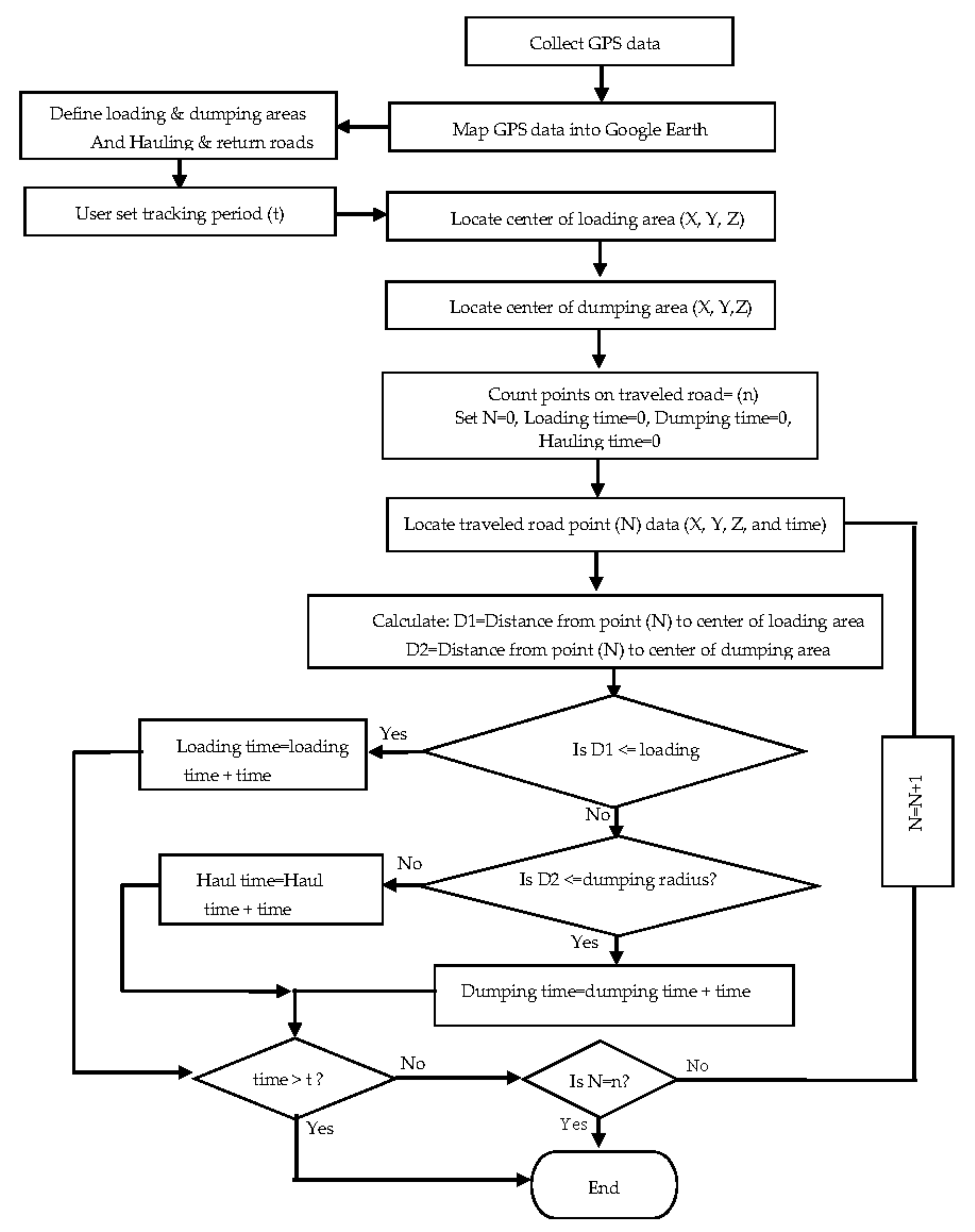
As presented in Figure 1, the proposed methodology incorporates five main components. They are GPS receivers, developed Graphical User Interface, Google Earth, developed algorithm of extracting activities durations’, and Fuzzy set computational algorithm for estimating the actual productivity of earthwork. The GPS receivers are used to collect data of the monitored equipment in real times. GUI is designed and developed to facilitate data entry for both graphical and non-graphical data. The GUI also automates data acquisition and analyzing the collected GPS data to extract the durations of loading, hauling, dumping, and returning activities. Google earth is used for a graphical presentation of the tracked equipment and for identifying loading, hauling, dumping, and returning activities. The algorithm of determining activities duration is developed to calculate the activities durations from the collected GPS data. The fuzzy set algorithm is used to enable project managers to define the uncertainties associated with activities durations and to estimate a fuzzy actual onsite productivity. It should be noted that the proposed methodology could also be used to select the most productive fleet among a set of alternative fleets. The following sections describe in detail the main process of the proposed methodology.
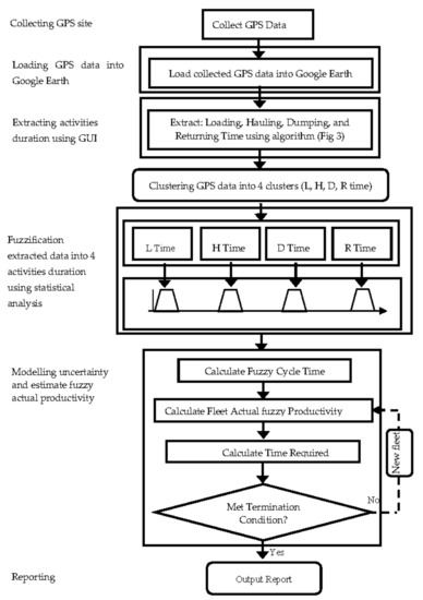
Figure 1.
Flow chart of the developed methodology.
2.1. Data Collection
The GPS is chosen for collecting data from a construction site for the purpose of measuring onsite actual productivity because [14]: (1) GPS gives plenty of information to track the operations of earthmoving as shown in Table 1; (2) Data collected by GPS in the form of time, speed, direction and latitude, longitude, altitude coordinates are correct and accurate; (3) the collected position data for different segments of travelled roads can be used to generate a road profile; and (4) the idle, haul, and maneuver times of the tracked truck can be easily determined from the collected GPS data.

Table 1.
Samples of collected GPS data.
For easiness and efficiency, only a receiver unit of GPS is attached to a truck to measure the productivity of entire fleet since all the involved trucks can be represented through cycle time of that truck. The GPS unit used in this study cost 370 Canadian dollars and the cost of the used storage server for the data was about 50 Canadian dollars/ month. The GPS unit is attached inside the truck cabinet.
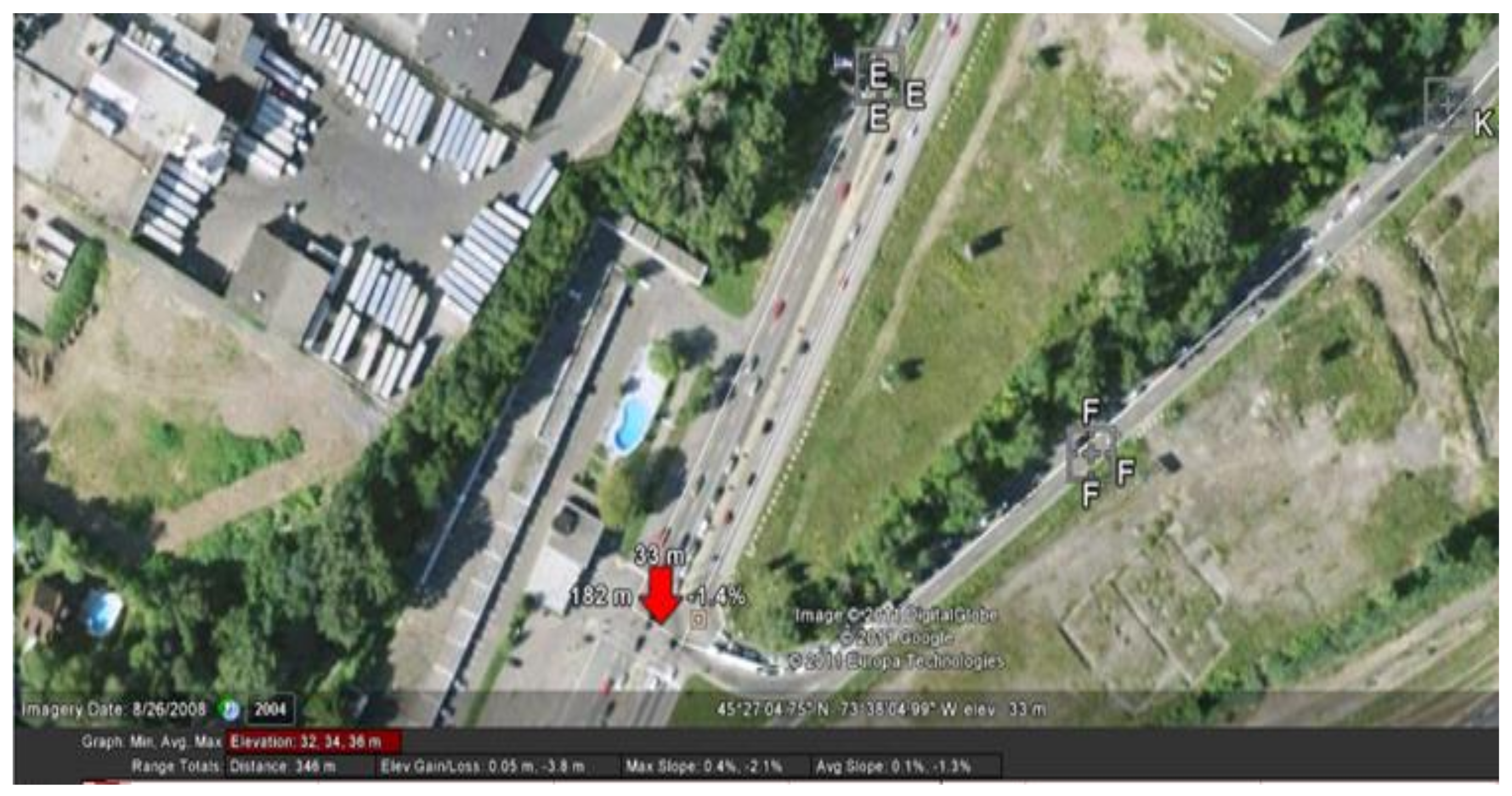
The GPS data was collected daily in short time interval at various times of the day to demonstrate actual conditions of construction site, and implicitly accounts for traffic and weather conditions. A sample of the collected GPS data is shown in Table 1. The collected GPS data were mapped in near real time via internet connection into Google Earth for graphical presentation and for extracting activity durations of the entire operation using the developed algorithm as presented in the following section. Figure 2 depicts the travelled road to the construction site of the example project as shown in Google Earth.

Figure 2.
View of traveled road of case project in Google Earth.
2.2. Extraction of Activities duration from GPS Data
After collecting and uploading of the collected GPS data of the tracked truck into google map, the developed methodology then fires a developed standalone graphical user interface (GUI) for extracting activities duration using the developed algorithm as presented in Figure 3. The extracting activities include (loading, travelling, dumping, and returning), which are then utilized to determine the truck cycle times. The following are the main five steps that summarize the process of extraction activities duration from the collected GPS Data:

Figure 3.
Extracting activities duration from collected GPS data.
- Uploading the collected GPS data into Google Earth.
- Locating and defining the loading and dumping sites on Google map using a developed drawing tool to facilitate the identification of departure and arrival times required to compute the truck cycle time. Here, the user on Google Earth needs to define locations of loading and dumping sites so that these locations can be recognized when the truck is in the loading or dumping sites. The coordinates of the identified loading and dumping area are saved in a central database in form of dbf format. The user can define several loadings and dumping sites dynamically as the work progress. Different shapes can be used to display loading and dumping sites to fit certain job site.
- Having defined the loading and dumping sites, the developed algorithm of extracting duration then extracts the coordination (XYZ) of positions on the traveled road from GPS data.
- Computing the distance between mid-points (center) of identified dumping and loading areas and the position of the point under consideration using Haversine formula [20]. Recognizing the location of the tracked truck based on the calculated distance in step 2. One of two conclusions can be reached; (1) If calculated distance is longer than the radius of dumping and loading sites, the truck is identified as in traveling or returning; (2) If the calculated distance is smaller than the specific radius of loading and dumping sites, the truck in this case would be within loading or dumping area. Dumping time can be determined as time illustrated when the truck is within the dumping site, and likewise loading time is computed as a time taken for the truck to stay in the loading area. Hauling and returning times were differentiated by the direction of the moving unit. If the direction was from the loading to the dumping area, time computed would be for hauling. Otherwise it would be for the returning time.
- Repeating step 4 till all locations on the travelled roads are identified. Table 2 depicts a sample of the extracted duration of cycle times of the case study project.
Table 2. Extracted cycle times.
- Clustering the extracted cycle times into four groups. Group four is selected to present the loading, dumping, hauling, and returning time of the tracked truck, which are the main components of the truck cycle time.
- Performing statistical analysis on the extracted durations includes calculating minimum, maximum, mean, and median of loading, dumping, hauling, and returning time of the tracked truck to form fuzzy numbers of the cycle time.
2.3. Modelling Uncertainty and Estimate Productivity
To model uncertainties associated with the extracted cycle times: loading (T1), traveling (T2), dumping (T3), and returning (T4) activities, the following steps are performed:
- Defining the functions of membership to the four fuzzy numbers (a, b, c, and d) based on computed mean, median, standard deviation, minimum, and maximum values. Mean and median were used to define the lower and upper modes (i.e., b and c) with full membership (i.e., f(x) = 1.0) and minimum and maximum were used to define lower and upper bounds (i.e., a and d) with no membership (i.e., f(x) = 0.0). The contractor can set different membership functions of the four activity durations, based on his/her judgment. In the example project provided in this paper trapezoidal and triangular shapes were used, with full membership at the median.
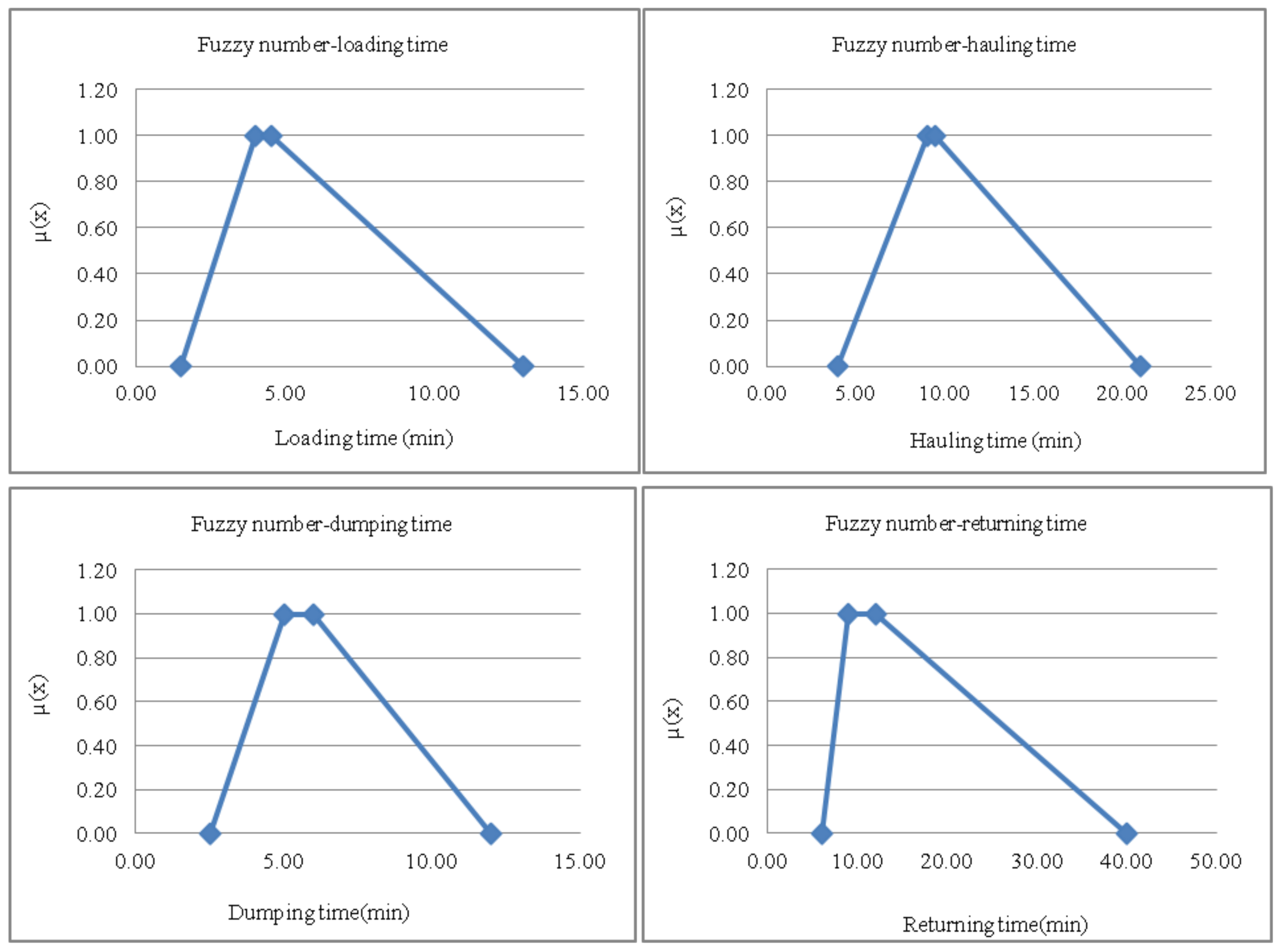
- Calculating the fuzzy cycle time of the monitored truck by adding the bases of the cycle time’s fuzzy numbers. Figure 4 illustrates the calculated fuzzy activity durations of the case project presented in this paper.
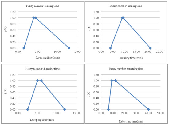 Figure 4. Fuzzy activity durations.
 - Defuzzifing the calculated fuzzy cycle time by calculating a crisp expected value of the cycle time through center of area (COA) technique [12].
- Calculating the fleet fuzzy onsite productivity based on the hauling unit’s fuzzy cycle time using Equation (1).where m = number of trucks model in the fleet being considered; nt is number of trucks of the same model in the fleet under consideration; Pa = estimated fleet productivity; FCT = the calculated fuzzy cycle time; Tc = the capacity of the truck of the same model taking into consideration the soil type; FF = adjustment factor that accounts for the fill factor which is relied upon soil type.
- Analyzing the calculated fuzzy cycle time and the estimated fleet fuzzy productivity, using a set of indices as described in the case project.
3. Case Project
The project is a new building constructed recently at Concordia University’s Loyola campus located west of the city of Montreal. The project involves the excavation of a basement that requires the use of excavator and many trucks in an urban area. The project was also analyzed earlier for estimating actual productivity using deterministic and probabilistic models to compare the outcomes of the methodology and the results generated by deterministic and probabilistic based models [7].
The fleet used in this project consists of an excavator and number of articulated trucks. Excavation soil was mainly sandy-clay. The foundation plans indicate that the average excavation depth is 7.70 m and the excavation area is approximately 1800 m2. To demonstrate the accuracy of the developed methodology, the estimated productivity was compared to the actual productivity achieved by the contractor onsite and it was also compared to those obtained by using deterministic and probabilistic based models [7].
Data of 104 truck cycles’ times in total were obtained from the collected GPS data. Table 2 depicts a sample of the extracted cycle times from the collected GPS data. The table shows a variation in the extracted cycle times. The variation occurs due to: (1) the project was constructed in an urban area in which the travel road was vulnerable to the blockage of traffic; (2) traffic may slow down due to weather conditions; (3) the project contains two dumping areas that were situated at various distances from the construction site. Table 3 depicts the calculated fuzzy numbers of activities durations.
Table 3.
Fuzzy numbers of activities durations.
3.1. Results and Discussions
To illustrate the features of the developed methodology in measuring actual onsite productivity of earthmoving operations, the productivity was first estimated as a crisp number and then as a fuzzy number and finally compared to the actual productivity the contractor achieved. The results provided by the developed tool is also compared to that obtained by deterministic and probabilistic models [15,19], respectively.
Trapezoidal and triangular membership functions were used to define the uncertainties associated with activity durations; respectively. In first case, activity durations (loading, hailing, dumping, and returning) were defined by trapezoidal fuzzy numbers. In the second case, activity durations were defined by triangular fuzzy numbers with their full membership at the median.
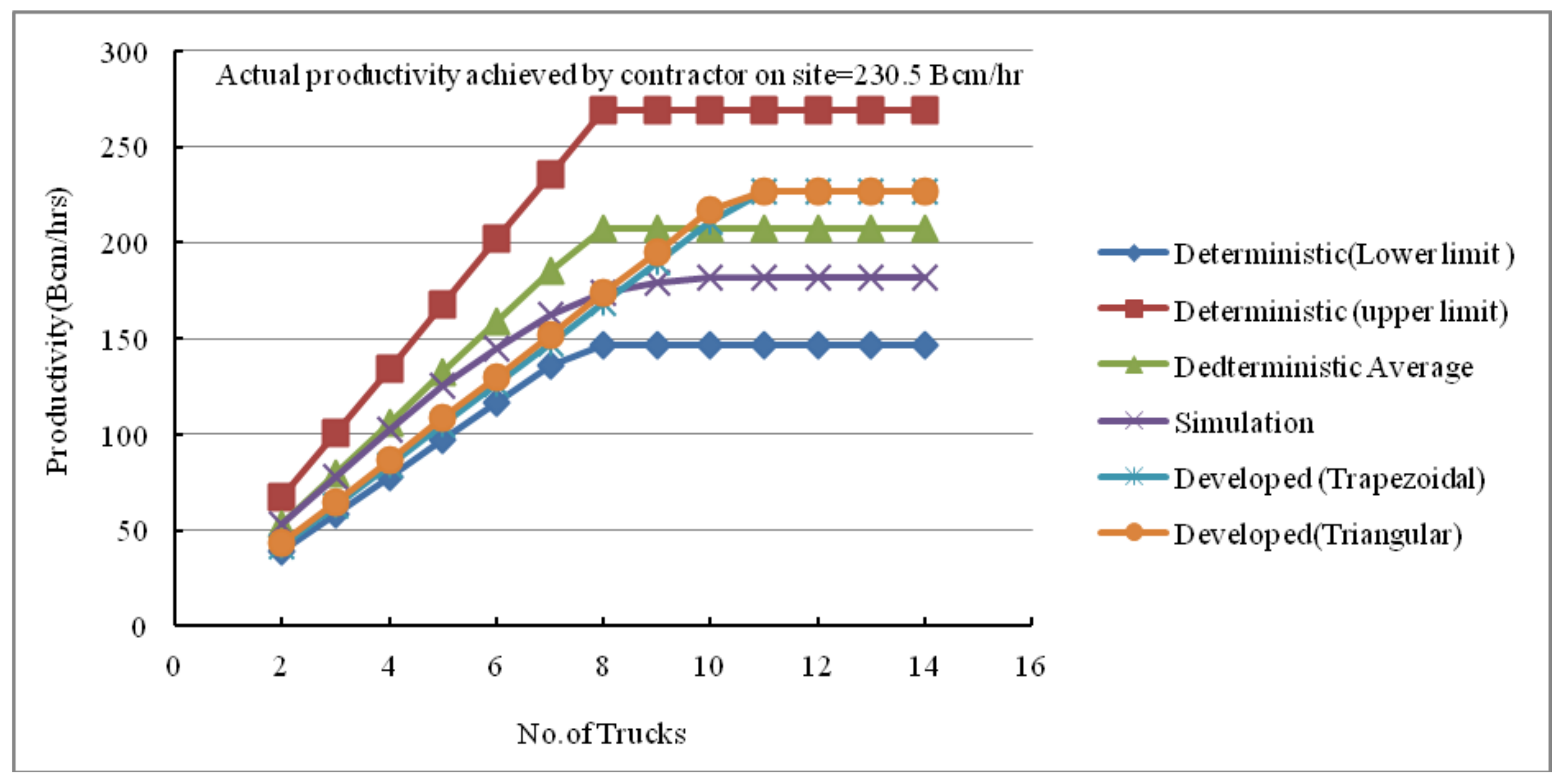
The number of trucks involved in the operations was varied and therefore the associated productivity was estimated to enable a comparison over a wide range of trucks used in Montaser et al. [7]. In addition, ambiguity, possibility, fuzziness measures, agreement index, and expected value are all used to assist in defining the uncertainty associated with the estimated productivity. Comparison of the outputs of the developed methodology to the actual productivity the contractor achieved and to those obtained by simulation-based model [15,19] is shown in Figure 5.
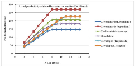
Figure 5.
Comparing the developed methodology with deterministic, and probabilistic models.
As presented in Figure 5, the estimated onsite productivity using the proposed methodology (trapezoidal and triangular numbers) is very close (identical) to what the contractor measured on site (226.63 Bcm/hr vs 230.5 Bcm/hr). In addition, it is closer to the average of the lower and upper deterministic estimates than that provided by the simulation based model as presented in Table 4. The productivity estimated by the developed methodology falls between the productivity estimated using simulation and the upper limit of the productivity estimated using the deterministic model. Table 4 depicts a comparison of the output of different methods for different fleet sizes.
Table 4.
Comparison of the Results (productivity estimation (Bcm/hr) for Different Fleet Size.
It is essential to note that using fuzzy numbers to model uncertainties associated with the duration of loading, traveling, dumping, and returning activities yields close results to those generated using simulations-based models. This makes the developed methodology a more practical tool. Comparing the outputs of the developed methodology to that of deterministic and simulation-based models, the following can be observed:
- The output of the developed methodology is very close to the actual productivity the contractor achieved and measured.
- The output of the developed methodology is in an agreement with the output of the simulation-based model for identifying the most productive fleet formation (11 trucks) required to serve an excavator.
- The developed methodology requires only a one step calculation to estimate productivity compared to that of simulation-based models, which need multi runs (e.g., 1000 iteration) to generate significant productivity estimates.
To provide interpretations to the obtained results, a set of measures and indices were used [21]. They are possibility measure, fuzziness (F), agreement Index and ambiguity (AG). Possibility measure is used to calculate feasibility of estimation of certain fleet productivity and/or cycle time. As an example, possibility measures that the truck cycle time is 22 min, as used in the deterministic model, and equals 0.8. The fuzzy number that has the possibility measurement of 1.0 is considered to be most plausible and feasible variable. Therefore, the most plausible and feasible truck cycle time is somewhere between 25–35 min.
The assessment of feasibility of productivity to be at a set crisp value or within a specific range is also carried out through the possibility measure. As shown in Figure 6, the calculated fuzzy productivity of the fleet that consists of one excavator and 11 trucks (most productive fleet formation) is (a = 86.00, b = 231.24, c = 287.36, d = 528.50) Bcm/hr. The possibility of the following two events are also examined:
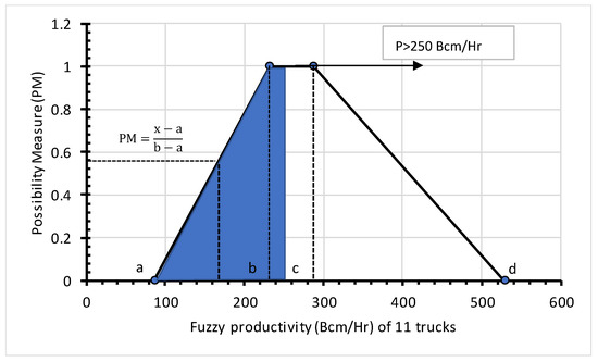
Figure 6.
Possibility measure of productivity event.
- The fleet productivity would be between 400 Bcm/hr and 500 Bcm/hr.
- Fleet productivity is exactly 300 Bcm/hr.
As it can be seen in Figure 6, the fuzzy productivity of the first event is expressed by four numbers (400, 400, 500, 500) and the fuzzy productivity in the second event is expressed as (300, 300, 300, 300). In the first case, the intersections are: {400|0.53, 400|0.53, 500|0.12, 500|0.12}, so in this case the probability that the productivity lies between 400 Bcm/hr and 500 Bcm/hr is 0.53. With respect to the second case which exactly 300 Bcm/hr; the assessment was made between two fuzzy events. The elements that fall into the intersection range and their degrees of membership include {300|0.95, 300|0.95, 300|0.95, 300|0.95} therefore the possibility of having productivity about 300 Bcm/hr is 0.95 (see Figure 6). According to the possibility measurement, it is clear that the most possible productivity rate of the fleet that consists of 11 trucks and one excavator, which is about 300 Bcm/hr. for the elements along with their related degree of membership.
Possibility measure gets its value through the highest membership function resulting from the area of intersection of the two events that are involved in the method. As in the case described above, calculating the possibility of the fleet productivity falls between 400 Bcm/hr and 500 Bcm/hr. In applying the possibility measure, the area of intersection is not accounted for. Considering that the possibility of the fleet productivity is between 400 and 500 Bcm/hr and that the fleet productivity is greater than 400 Bcm/hr, the PM of these two scenarios are almost equivalent (PM = 0.53), although the intersection area of the second case is greater than the first one.
On the other side, the Agreement Index accounts for the intersection area. For the same example above, the possibility the fleet productivity falls between 400 and 500 Bcm/hr is 0.53, but 0.95 for the fleet productivity being greater than 300 Bcm/hr. The agreement index, on the other hand is 0.13 for the first case and 0.43 for the second. In addition, it can be seen that the possibility of the fleet productivity being greater than 250 Bcy/hr is higher than these two cases; with possibility measures of 1.0 and an agreement index of 0.63.
Table 4, Table 5 and Table 6 show a comparison between the output of the developed methodology and each of the deterministic and probabilistic based models used in estimating onsite productivity. The comparison reveals that developed methodology yields not only closer results to the productivity actually achieved onsite, but it also suggests certain effective tools to contractors to assess the possibility of achieving a certain productivity value; which cannot be determined using any probability-based analysis, such as simulation as depicted in Table 6. For example, the possibility of the productivity being 300 Bcm/hr is 0.9, whereas using probabilistic analysis this crisp number cannot be evaluated.
Table 5.
Comparison of the results.
Table 6.
Evaluation of different measures applied to estimated productivity.
3.2. Features of the Proposed Methodology
The developed methodology has a number of features: (1) it yields results that are close to the actual productivity achieved by contractors; (2) it is simpler than simulation based modes; (3) It does not require specialized skills; (4) it allows the users to conduct a risk analysis assessment in a much easier way; (5) it allows the users to perform alternative selections of different outputs using measure indices; and (6) it is an inexpensive tool for comparing the commercial systems described earlier, (7) the developed methodology can be used by small to average size contractors who cannot afford expensive commercial tracking systems.
3.3. Limitations of the Study and Recommendation of Future Work
This study is limited to fleet configuration and consists of an excavator at time. It also assumes that the tracked fleet consists of trucks of the same size, which may not always be true. In such cases, more GPS receivers should be attached to all trucks in the fleet, which makes the proposed methodology costly. The developed approach is limited to open cut excavation that involves only the use of fleets consisting of an excavator and trucks.
As for future research, estimating onsite productivity of other fleet configurations, such as those that consist of dozers and scrapers, may need the combination of GPS and other technologies such as RFID and other remote sensing technologies. The proposed methodology can be improved if it integrates with BIM for updating the actual progress on 3D models for the work under consideration. It also can be integrated with sensor technologies to handle ever excavation of underground earth work and not only open cut excavation.
4. Conclusions
This paper presents a methodology that applies GPS data and fuzzy numbers for estimating onsite productivity of excavation work in near real time in an urban area. The developed methodology can provide the project management team with a user-friendly method to estimate the onsite productivity of excavation work. The proposed methodology can provide an accurate estimation with less effort and time and with a cheaper method when compared with sophisticated and expensive commercial systems. Results obtained through the application of the developed methodology were compared to actual onsite productivity achieved by a contractor on a construction site and compared to those provided by deterministic and probabilistic based methods. The results indicate that the application of fuzzy numbers to model uncertainties associated with activity duration can provide more realistic results than those modeling uncertainties using simulations.
Funding
This research received no external funding.
Conflicts of Interest
The authors declare no conflicts of interest.
References
- Zhang, C.; Hammad, A.; Bahnassi, H. Collaborative multi-agent systems for construction equipment based on real-time field data capturing. J. Inf. Technol. Constr. 2009, 14, 204–228. [Google Scholar]
- Christian, J.; Xie, T. Improving earthmoving estimation by more realistic knowledge. Can. J. Civ. Eng. 1996, 23, 250–259. [Google Scholar] [CrossRef]
- Paek, J.; Lee, Y.; Ock, J. Pricing construction risk: Fuzzy set theory application. J. Constr. Eng. Manag. 1993, 119, 743–756. [Google Scholar] [CrossRef]
- Tam, C.M.; Tong, T.K.L.; Tse, S.L. Artificial neural networks model for predicting excavator productivity. Eng. Constr. Archit. Manag. 2002, 2002, 446–452. [Google Scholar] [CrossRef]
- Montaser, A.; Moselhi, O. RFID+ for tracking earthmoving operations. In Proceedings of the Construction Research Congress 2012, West Lafayette, IN, USA, 21–23 May 2012; pp. 1011–1020. [Google Scholar] [CrossRef]
- Montaser, A.; Azram, R.; Moselhi, O. Experimental study for efficient use of Rfid in construction. In Proceedings of the 30th ISARC, Montréal, QC, Canada, 11–15 August 2013; pp. 618–625. [Google Scholar]
- Montaser, A.; Bakry, I.; Alshibani, A.; Moselhi, O. Estimating productivity of earthmoving operations using spatial technologies. Can. J. Civ. Eng. 2012, 39, 1072–1082. [Google Scholar] [CrossRef]
- Montaser, A.; Moselh, O. Truck+ for earthmoving operations. J. Inf. Technol. Constr. 2014, 19, 412–433. [Google Scholar]
- Rashidi, A.; Nejad, H.R.; Maghiar, M. Productivity estimation of bulldozers using generalized linear mixed models. KSCE J. Civ. Eng. 2014, 18, 1580–1589. [Google Scholar] [CrossRef]
- Montaser, A.; Moselhi, O. Automated site data acquisition technologies for construction progress reporting. In Proceedings of the CSCE 2014 General Conference—Congrès général 2014 de la SCGC, Halifax, UK, 28–31 May 2014. [Google Scholar]
- Hajjar, D.; AbouRizk, S. Unified modeling methodology for construction simulation. J. Constr. Eng. Manag. 2002, 128, 174–185. [Google Scholar] [CrossRef]
- Shaheen, A.; Fayek, A.; AbouRizk, S. Fuzzy numbers in cost range estimating. J. Constr. Eng. Manag. 2007, 133, 325–334. [Google Scholar] [CrossRef]
- Chung, T. Simulation—Based Productivity Modeling for Tunnel Construction Operations. Ph.D. Thesis, Department of Civil and Environmental Engineering, University of Alberta, Edmonton, AB, Canada, 2007. [Google Scholar]
- Kannan, G. A Methodology for the Development of a Production Experience Database for Earthmoving Operations Using Automated Data Collection. Ph.D. Thesis, Department of Civil Engineering, Faculty of the Virginia Polytechnic Institute and State University, Blacksburg, VA, USA, 1999. [Google Scholar]
- Montaser, A.; Moselhi, O. Tracking scraper-pusher fleet operations using wireless technologies. In Proceedings of the 4th Construction Specialty Conference, Montréal, QC, Canada, 29 May–1 June 2013. [Google Scholar]
- Yang, Y.; Farrell, J.; Barth, M. High-accuracy, high-frequency differential carrier phase GPS aided low-cost INS. In Proceedings of the IEEE Position, Location and Navigation Symposium, San Diego, CA, USA, 13–16 March 2000. [Google Scholar]
- Navon, R.; Goldschmidt, E. Monitoring labor inputs: Automated-data collection model and enabling technologies. J. Autom. Constr. 2002, 12, 185–199. [Google Scholar] [CrossRef]
- Shi, H.; Qiao, D. Experimental study on accuracy of GPS positioning. Appl. Mech. Mater. 2013, 263–266, 346–349. [Google Scholar] [CrossRef]
- Montaser, A.; Bakry, I.; Alshibani, A.; Moselhi, O. Estimating productivity of earthmoving operations using spatial technologies. In Proceedings of the 3rd International/9th Construction Specialty Conference, Ottawa, ON, Canada, 14–17 June 2011. [Google Scholar]
- Sinnott, W.W. Virtues of the Haversine. Sky Telesc. 1984, 68, 159. [Google Scholar]
- Zadeh, L. Fuzzy Sets as a basis for a theory of possibility. Fuzzy Sets Syst. 1978, 1, 3–28. [Google Scholar] [CrossRef]


© 2018 by the author. Licensee MDPI, Basel, Switzerland. This article is an open access article distributed under the terms and conditions of the Creative Commons Attribution (CC BY) license (http://creativecommons.org/licenses/by/4.0/).