Energetic, Cost, and Comfort Performance of a Nearly-Zero Energy Building Including Rule-Based Control of Four Sources of Energy Flexibility

 ,
,  ,
,
Abstract
1. Introduction
2. Research Method
2.1. Building
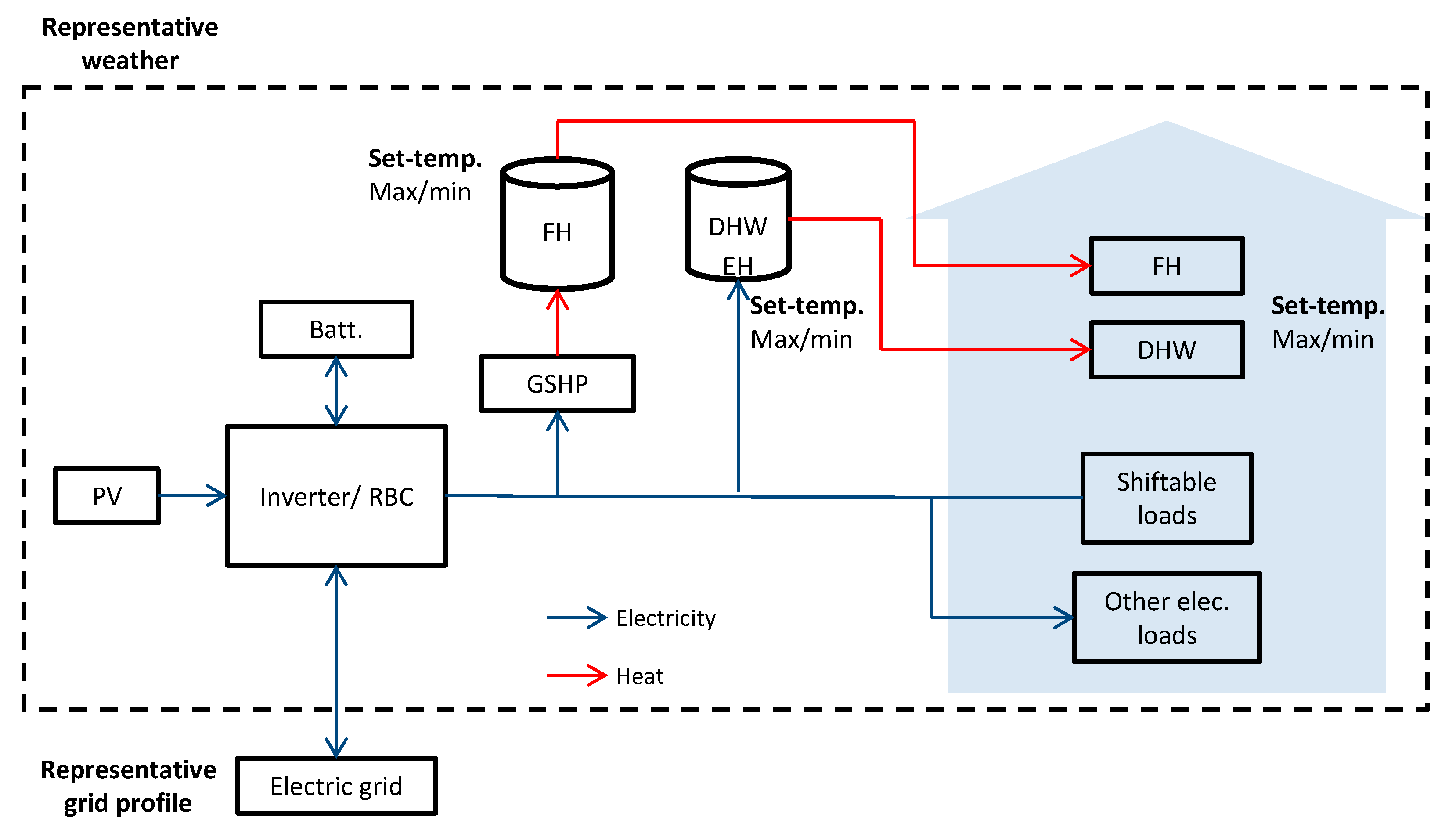
2.2. Energy System
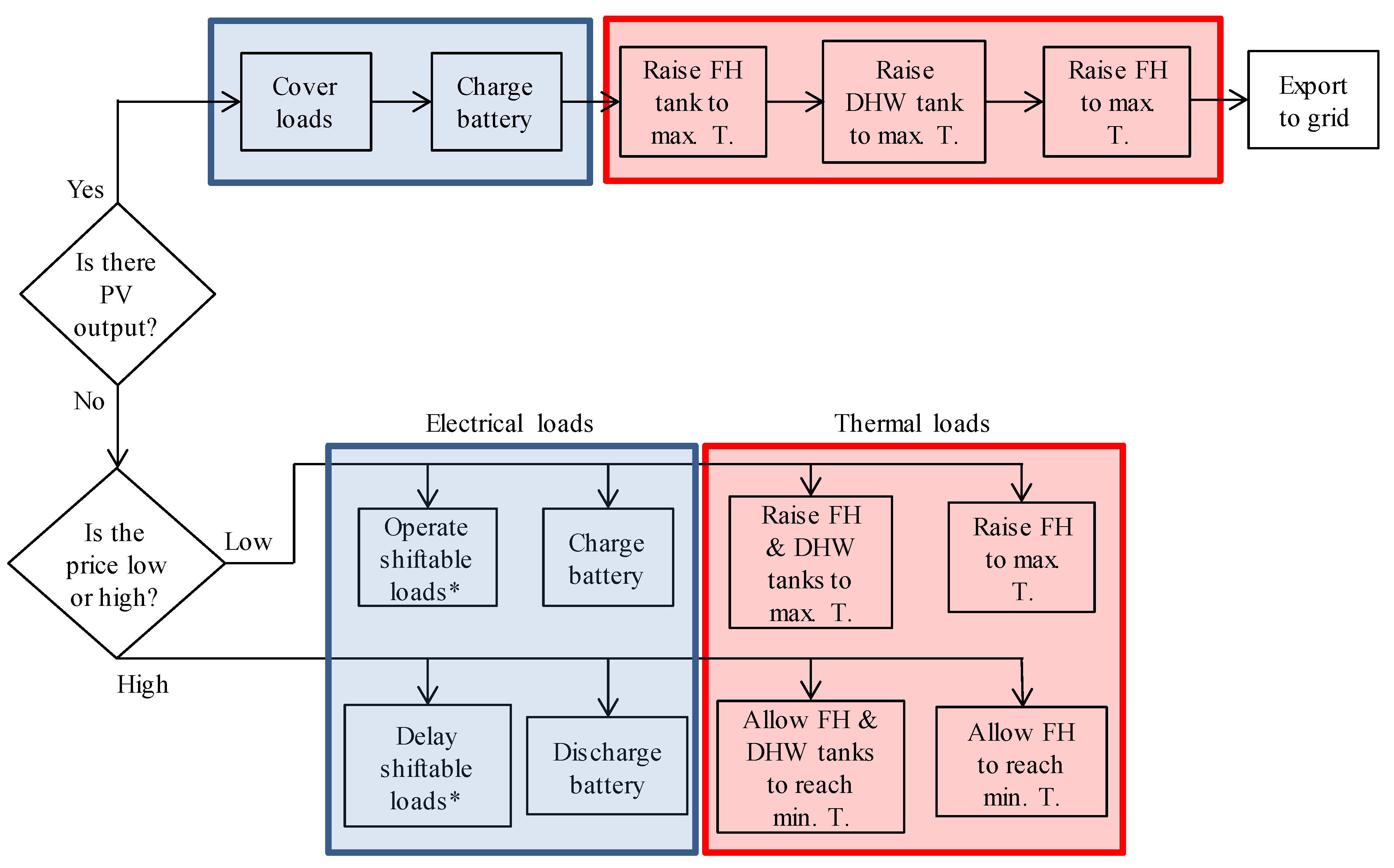
2.3. Control Strategies
2.4. Shiftable Machine Loads
2.5. Set-Point Temperatures and Comfort Evaluation
2.6. Indicators
2.7. Simulation
2.8. Reference Case
3. Results
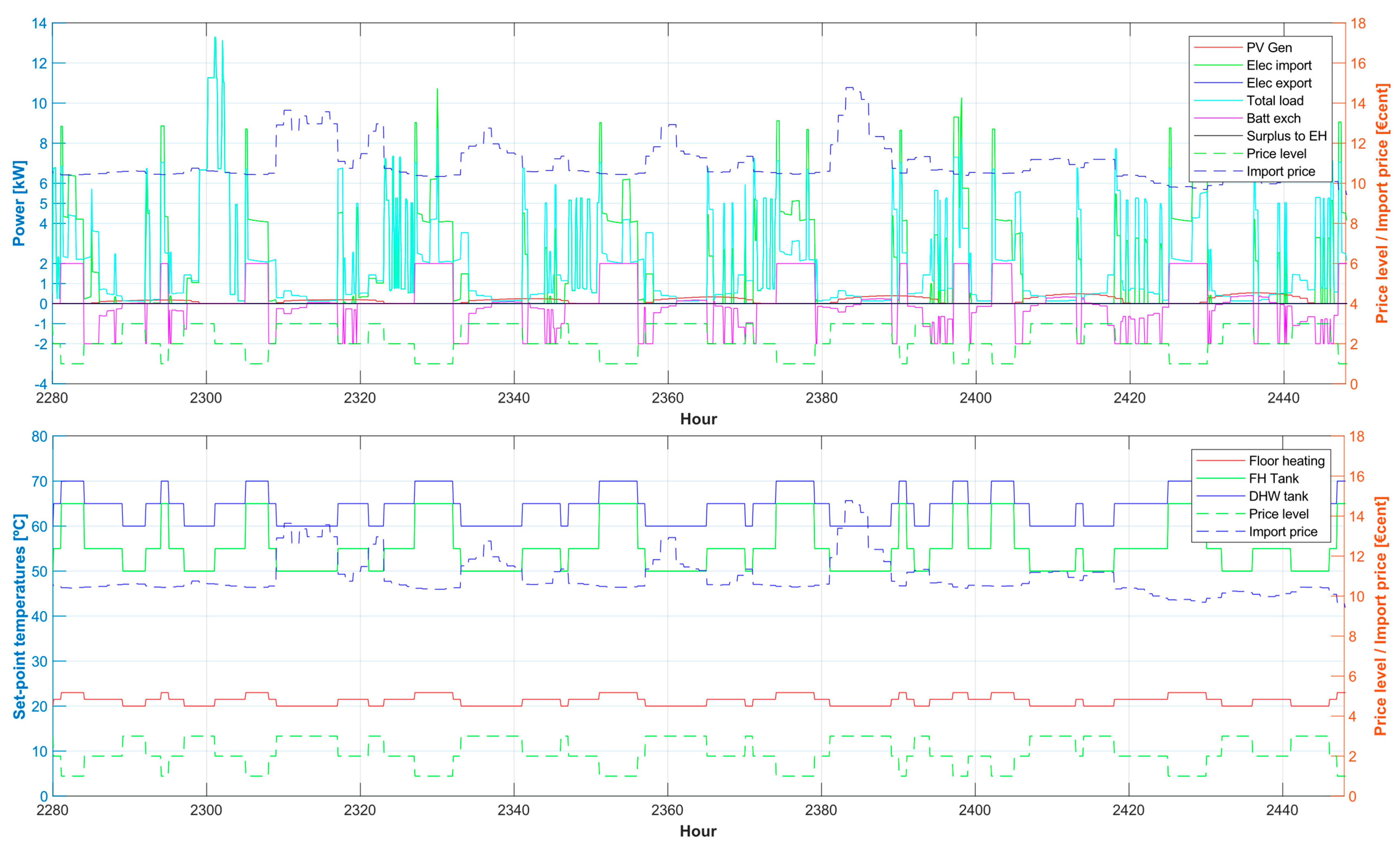
3.1. Operation of the RBC
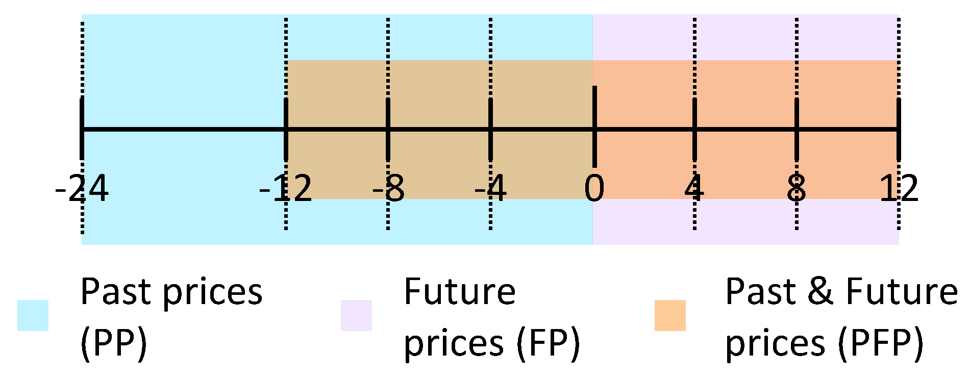
3.2. Price Categorization
3.3. Performance of the Energy Flexibility Actions
3.4. Comfort Evaluation
4. Discussion
4.1. On Price Categorization
4.2. On the Performance of the Energy Flexibility Actions
4.3. On the Comfort Evaluation
4.4. Single Action Performance
5. Conclusions
- The energy matching and flexibility actions provided a decrease of up to 4% in annual energy costs, yet risk increasing the cost by 9% when implemented improperly. Shifting electricity consumption to low electricity prices may be counterproductive if the savings are offset by the increase in the energy demand. Thus, improved flexibility may lead to monetary losses if the control parameters are not chosen carefully.
- Price-based management of the battery, modulation of the set-point temperature of the storage tanks, and modulation of the floor heating offer roughly the same potential for cost savings. Price-based shifting of the operation of the washing machine, dryer and dishwasher did not provide cost savings in this study. Support mechanisms are needed to make load-shifting more attractive for the end-user. As well, energy matching is negatively affected by the price-based management of the battery. Thus, this flexibility action is detrimental for energy self-consumption.
- The flexibility actions lead to a decrease in the comfort levels inside the building. Namely, the FH flexibility actions with an in-slab floor heating system lead to slow changes in the indoor temperature, which is detrimental for temperature-range based comfort indicators but beneficial to avoid sudden temperature changes.
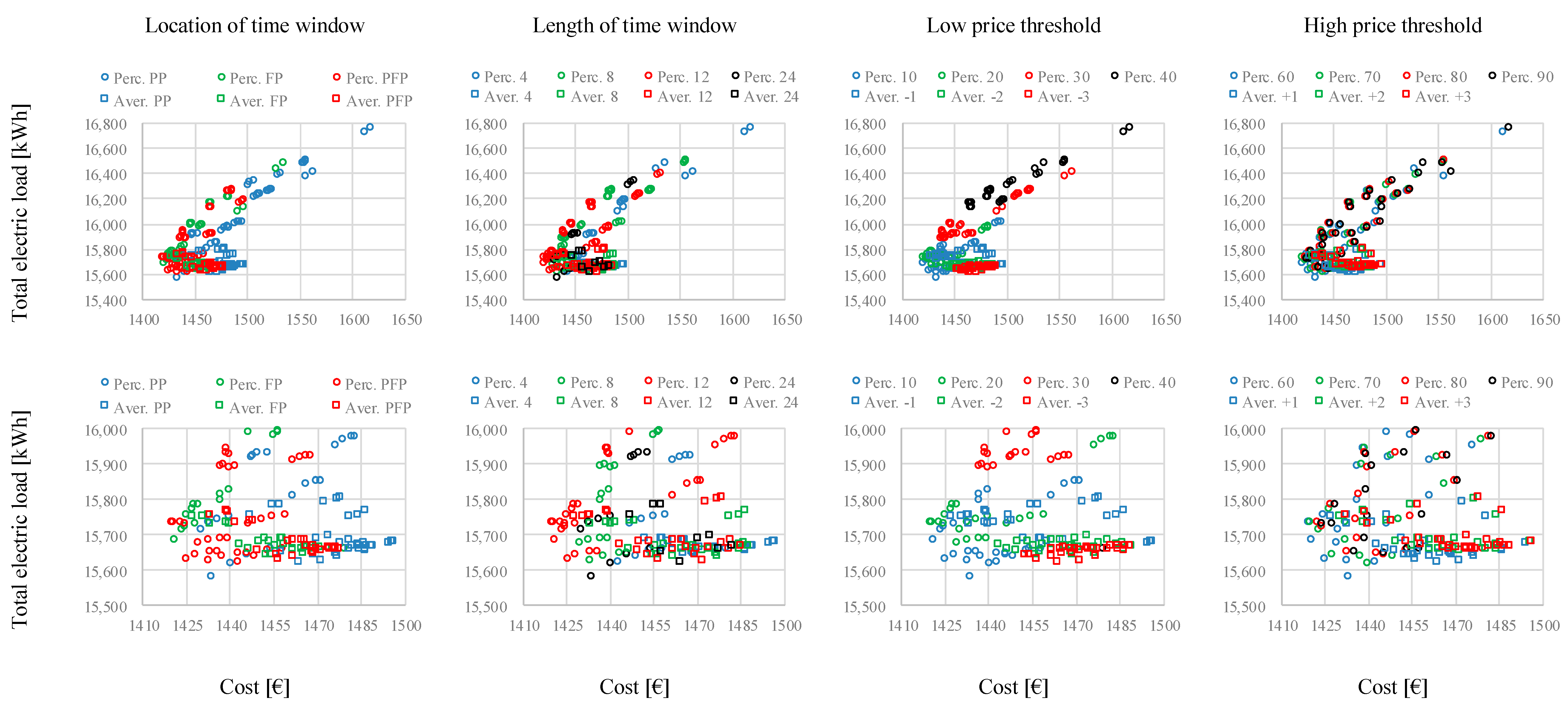
- Categorizing the electricity prices based on percentiles leads to more frequent reactions to price changes than categorizing based on a moving average and a fixed range; that is, the percentiles approach leads to a more frequent implementation of the flexibility actions and thus to a wider range of results. Twelve-hours windows for evaluation of electricity prices show better results than shorter windows, as more price information helps to better classify prices as low or high.
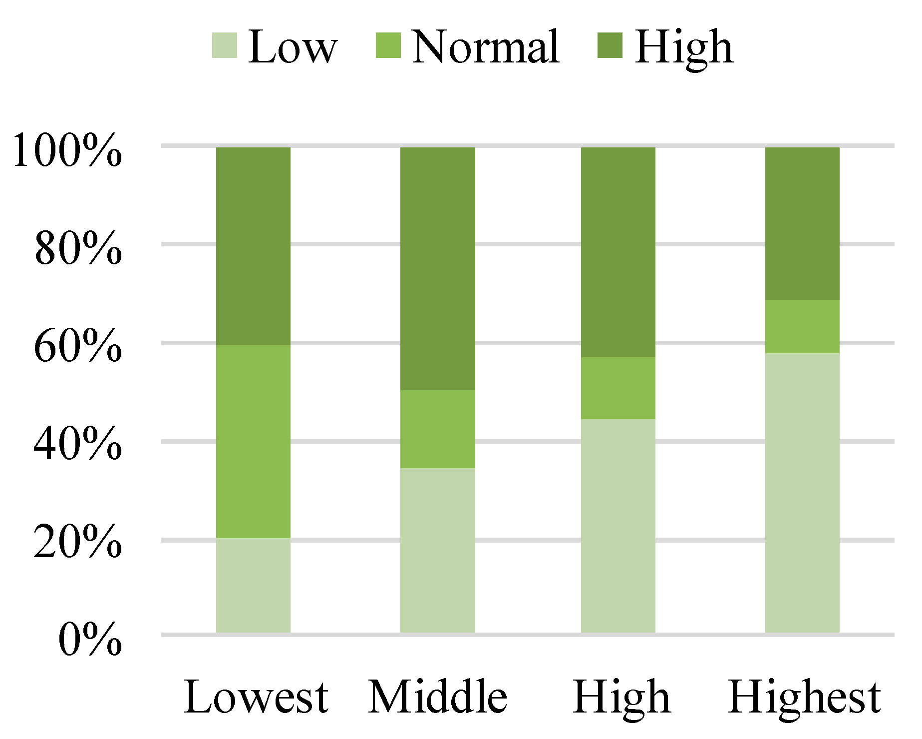
- The low-price threshold shows more influence on the annual energy cost than the high-price threshold. A high percentage of hours categorized as low-price leads to increased costs and loads, while frequent fluctuations between low, normal, and high categorization enhance the charge/discharge actions.
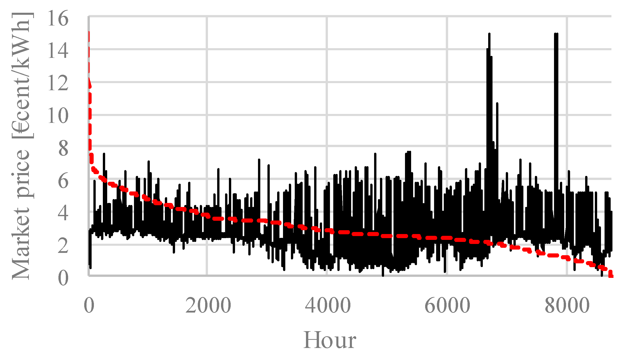
- The behavior of the hourly energy price curve limits the savings potential of the energy management actions. Namely, short amplitude of price oscillations leads to limited savings potential, and infrequent drops in prices make energy charging actions less consequential.
- Modulating the set-point temperature of the FH tank can lead to variations in the COP of the GSHP, as it depends of the temperature of the water stored inside the tank. Particularly, elevating the temperature inside the tank decreases the COP of the GSHP, and thus increases its electricity demand.
Author Contributions
Funding
Conflicts of Interest
Abbreviations
| COP | Coefficient of performance |
| DHW | Domestic hot water |
| DR | Demand response |
| FH | Floor heating |
| FP | Future prices |
| GSHP | Ground-source heat pump |
| HEP | Hourly electricity prices |
| HWST | Hot water storage tank |
| MPC | Model predictive control |
| OEF | Onsite energy fraction |
| OEM | Onsite energy matching |
| PCAO | Parameterized Cognitive Adaptive Optimization |
| PFP | Past and future prices |
| PP | Past prices |
| PV | Photovoltaic |
| RBC | Rule-based control |
References
- European Commission. Buildings. 2017. Available online: https://ec.europa.eu/energy/en/topics/energy-efficiency/buildings (accessed on 14 February 2018).
- Haider, H.T.; See, O.H.; Elmenreich, W. A review of residential demand response of smart grid. Renew. Sustain. Energy Rev. 2016, 59, 166–178. [Google Scholar] [CrossRef]
- Nolan, S.; O’Malley, M. Challenges and barriers to demand response deployment and evaluation. Appl. Energy 2015, 152, 1–10. [Google Scholar] [CrossRef]
- Alimohammadisagvand, B.; Jokisalo, J.; Sirén, K. Comparison of four rule-based demand response control algorithms in an electrically and heat-pump heated residential building. Appl. Energy 2018, 209, 167–179. [Google Scholar] [CrossRef]
- Hoon Yoon, J.; Bladick, R.; Novoselac, A. Demand response for residential building based on dynamic price of electricity. Energy Build. 2014, 80, 531–541. [Google Scholar] [CrossRef]
- Christantoni, D.; Oxizidis, S.; Flynn, D.; Finn, D. Implementation of demand response strategies in a multi-purpose commercial building using a whole-building simulation model approach. Energy Build. 2016, 131, 76–86. [Google Scholar] [CrossRef]
- Fotouhi Ghazvini, M.A.; Soares, J.; Abrishambaf, O.; Castro, R.; Vale, Z. Demand response implementation in smart households. Energy Build. 2017, 143, 129–148. [Google Scholar] [CrossRef]
- Baldi, S.; Karagevrekis, A.; Michailidis, I.; Kosmatopoulos, E. Joint energy demand and thermal comfort optimization in photovoltaic-equipped interconnected microgrids. Energy Convers. Manag. 2015, 101, 352–363. [Google Scholar] [CrossRef]
- Michailidis, I.; Baldi, S.; Pichler, M.; Kosmatopoulos, E.; Santiago, J. Proactive control for solar energy exploitation: A german high-inertia building case study. Appl. Energy 2015, 155, 409–420. [Google Scholar] [CrossRef]
- Neves, D.; Pina, A.; Silva, A. Demand response modeling: A comparison between tools. Appl. Energy 2015, 156, 288–297. [Google Scholar] [CrossRef]
- Knudsen, M.D.; Petersen, S. Demand response potential of model predictive control of space heating based on price and carbon dioxide intensity signals. Energy Build. 2016, 125, 196–204. [Google Scholar] [CrossRef]
- Péan, T.Q.; Ortiz, J.; Salom, J. Impact of Demand-Side Management on Thermal Comfort and Energy Costs in a Residential nZEB. Buildings 2017, 7, 37. [Google Scholar] [CrossRef]
- Le Dréau, J.; Heiselberg, P. Energy flexibility of residential buildings using short term heat storage in the thermal mass. Energy 2016, 111, 991–1002. [Google Scholar] [CrossRef]
- Oldewurtel, F.; Sturzenegger, D.; Morari, M. Importance of occupancy information for building climate control. Appl. Energy 2013, 101, 521–532. [Google Scholar] [CrossRef]
- Oldewurtel, F.; Parisio, A.; Jones, C.; Gyalistras, D.; Gwerder, M.; Stauch, V.; Lehmann, B.; Morari, M. Use of model predictive control and weather forecasts for energy efficient building climate control. Energy Build. 2012, 45, 15–27. [Google Scholar] [CrossRef]
- Kilpeläinen, S.; Lu, M.; Cao, S.; Hasan, A.; Chen, S. Composition and operation of a semi-virtual renewable energy-based building emulator. Future Cities Environ. 2018, 4, 1. [Google Scholar] [CrossRef]
- Finnish Ministry of Environment, Department of the Built Environment. D3 Suomen rakentamismääräyskokoelma [National Building Code of Finland D3]. 2011. Available online: http://www.finlex.fi/data/normit/37188/D3-2012_Suomi.pdf (accessed on 18 April 2018).
- Laitinen, A.; Shemeikka, J. RET—PIENTALON MÄÄRITTELY (Definition of Detached House); VTT Construction and Municipal Engineering: Espoo, Finland, 2005. (In Finnish) [Google Scholar]
- Cao, S.; Hasan, A.; Sirén, K. Analysis and solution for renewable energy load matching for a single-family house. Energy Build. 2013, 65, 398–411. [Google Scholar] [CrossRef]
- Cao, S.; Hasan, A.; Sirén, K. On-site energy matching indices for buildings with energy conversion, storage and hybrid grid connections. Energy Build. 2013, 64, 423–438. [Google Scholar] [CrossRef]
- Finnish Ministry of Environment, Department of the Built Environment. D5 Suomen rakentamismääräyskokoelma [National Building Code of Finland D5]. 2012. Available online: http://www.ym.fi/fi-FI/Maankaytto_ja_rakentaminen/Lainsaadanto_ja_ohjeet/Rakentamismaarayskokoelma/Energiatehokkuus (accessed on 18 April 2018).
- NordPool. Day-ahead Market. Available online: https://www.nordpoolgroup.com/the-power-market/Day-ahead-market/ (accessed on 24 August 2018).
- Finnish Society of Indoor Air Quality and Climate. Classification of Indoor Environment 2008. Available online: https://www.aecb.net/knowledgebase/publisher/finnish-society-of-indoor-air-quality-and-climate/ (accessed on 18 April 2018).
- ASHRAE. ANSI/ASHRAE Standard 55-2010 Thermal Environmental Conditions for Human Occupancy; ISSN 1041-2336; ASHRAE: New York, NY, USA, 2010. [Google Scholar]
- Manrique Delgado, B.; Cao, S.; Tuominen, P.; Hasan, A.; Jokinen, J. Energy Generation and Matching in a Net Zero-Energy Building in Finland; CIB World Building Congress: Tampere, Finland, 2016. [Google Scholar]
- Le Dréau, J. Demand-Side Management of the Heating Need in Residential Buildings. CLIMA 2016. In Proceedings of the 12th REHVA World Congress, Aalborg, Denmark, 22–25 May 2016. [Google Scholar]
- Finnish Meteorological Institute. Download Observations. Available online: http://en.ilmatieteenlaitos.fi/download-observations#!/ (accessed on 20 February 2018).
- NordPool. Historical Market Data. Available online: https://www.nordpoolgroup.com/historical-market-data/ (accessed on 23 March 2018).
- Caruna Oy. Network Service Fees. Available online: https://www.caruna.fi/asiakaspalvelu/hinnastot-and-sopimusehdot/sahkonsiirronhinta (accessed on 1 June 2016).
- Péan, T.Q.; Torres, B.; Salom, J.; Ortiz, J. Representation of daily profiles of building energy flexibility. In Proceedings of the eSim 2018, the 10th conference of IBPSA-Canada, Montréal, QC, Canada, 9–13 May 2018. [Google Scholar]


| Feature | Units | Value | |
|---|---|---|---|
| U-values | Walls | 0.169 | |
| Roof | 0.279 | ||
| Floor | 0.79 | ||
| Windows | 0.7 | ||
| Soil layer below ground | 0.16 | ||
| Dimensions | Net area | 150 | |
| Air volume | 375 | ||
| Ventilation | Air exchange rate | 0.4 | |
| Heat recovery efficiency | % | 70 | |
| Energy demand | Heating demand * | 56.2 | |
| DHW demand | 0.6 | ||
| Lighting | 7.01 | ||
| Appliances | 15.8 | ||
| Shiftable machine load | Dec, Jan, Feb | Mar, Apr, May | Jun, Jul, Aug | Sep, Oct, Nov |
|---|---|---|---|---|
| Dishwasher | Mon, Wed, Thu, Sat, Sun 20:00 to 06:00 | Mon, Wed, Thu, Sat, Sun 20:00 to 06:00 | Mon, Wed, Thu, Sat, Sun 20:00 to 06:00 | Mon, Wed, Thu, Sat, Sun 20:00 to 06:00 |
| Washing machine | Tue, Wed, Thu, Sat, Sun 20:00 to 06:00 | Tue, Wed, Thu, Sat, Sun 20:00 to 06:00 | Tue, Thu, Sat 20:00 to 06:00 | Tue, Wed, Thu, Sat, Sun 20:00 to 06:00 |
| Clothes dryer | Tue, Wed, Thu, Sat, Sun 06:00 to 10:00 | Tue, Wed, Thu, Sat, Sun 06:00 to 10:00 | Not used | Tue, Wed, Thu, Sat, Sun 06:00 to 10:00 |
| Tank | PV Excess | Electricity Price Category | ||
|---|---|---|---|---|
| Low | Normal | High | ||
| FH | 70 °C | 65 °C | 55 °C | 50 °C |
| DHW | 90 °C | 70 °C | 65 °C | 60 °C |
| Heating in conditioned areas | for , 27 °C for | 21.5 °C | 20 °C | |
| Period (hours) | 0.25 | 0.5 | 1 | 2 | 4 |
|---|---|---|---|---|---|
| Maximum operative temperature change allowed (°C) | 1.1 | 1.7 | 2.2 | 2.8 | 3.3 |
| Case | Description | Cost (€) | Tot. Load (kWh) | Net elec. exch. (kWh) | OEM | OEF | |||
|---|---|---|---|---|---|---|---|---|---|
| Lowest | Perc. PFP 12 h, Low: 20, High: 60 | 1420 | 15,734 | 13,730 | 1.00 | 0.13 | 0.55 | 219 | 97% |
| Middle | Perc. FP 8 h, Low: 40, High: 60 | 1481 | 16,213 | 14,222 | 0.98 | 0.12 | 0.55 | 710 | 92% |
| High | Perc. PP 4 h, Low: 20, High: 60 | 1556 | 16,374 | 14,324 | 0.98 | 0.12 | 0.82 | 813 | 90% |
| Highest | Perc. PP 4 h, Low: 40, High: 70 | 1617 | 16,759 | 14,676 | 0.97 | 0.12 | 0.89 | 1164 | 86% |
| Reference | - | 1481 | 15,664 | 13,511 | 1.00 | 0.14 | - | - | - |
| Management actions | Case | ||||
|---|---|---|---|---|---|
| PV Output | Reference | Lowest | Middle | High | Highest |
| Cover the electrical loads | 1356 | 1320 | 1200 | 1327 | 1244 |
| Charge the battery | 837 | 729 | 480 | 411 | 293 |
| Charge FH tank to max | 0 | 0 | 16 | 16 | 67 |
| Charge DHW tank to max | 0 | 90 | 294 | 241 | 327 |
| Raise FH set to max | 0 | 0 | 0 | 0 | 0 |
| Export | 0 | 6 | 35 | 36 | 56 |
| Price-Based Management | Reference | Lowest | Middle | High | Highest |
| High prices | |||||
| Shift appliances a | - | 1429 | 1429 | 591 | 731 |
| Use the battery | - | 1380 | 3023 | 1851 | 1308 |
| Discharge tanks to min. | - | 881 | 1234 | 318 | 85 |
| Lower FH set to min. | - | 4972 | 5677 | 4984 | 4390 |
| Low prices | |||||
| Shift appliances a | - | 1429 | 1429 | 591 | 731 |
| Charge the battery | - | 3074 | 3580 | 2298 | 1695 |
| Charge tanks to max. | - | 2103 | 3584 | 3991 | 4541 |
| Raise FH set to max. | - | 5646 | 6993 | 6268 | 5920 |
| Disch. batt. w. normal prices | - | 2233 | 836 | 715 | 570 |
| Case | Zone | S2, in % | Drifts and Ramps (h) (0.25/0.5/1/2/4) |
|---|---|---|---|
| Lowest | Bed SW | 56 | 0.2/0/0/0/0 |
| Bed NE | 56 | 0.9/1/0.7/0.8/0.2 | |
| Bed NW | 53 | 0.8/1/0.9/0.9/0.1 | |
| Liv. & Kit. | 72 | 0/0/0.3/0/0 | |
| Highest | Bed SW | 49 | 0.2/0/0/0/1.1 |
| Bed NE | 48 | 0.9/1/0.7/0.8/0.2 | |
| Bed NW | 49 | 0.7/1/0.9/1/0.2 | |
| Liv. & Kit. | 57 | 0/0/0.3/0/0 | |
| Reference | Bed SW | 7 | 0.2/0/0/0/0 |
| Bed NE | 0 | 0.9/1/0.7/0.8/0.2 | |
| Bed NW | 0 | 0.8/1/0.9/1/0.2 | |
| Liv. & Kit. | 9 | 0/0/0.3/0/0 |
| Case | Cost (€) | Tot. Load (kWh) | Net elec. exch. (kWh) |
|---|---|---|---|
| Tanks | 1461 | 15,799 | 13,648 |
| FH | 1465 | 15,693 | 13,542 |
| Shiftable machine loads | 1480 | 15,661 | 13,508 |
| Battery | 1460 | 15,664 | 13,664 |
| Lowest cost | 1420 | 15,734 | 13,730 |
| Reference | 1481 | 15,664 | 13,511 |
© 2018 by the authors. Licensee MDPI, Basel, Switzerland. This article is an open access article distributed under the terms and conditions of the Creative Commons Attribution (CC BY) license (http://creativecommons.org/licenses/by/4.0/).
Share and Cite
Manrique Delgado, B.; Ruusu, R.; Hasan, A.; Kilpeläinen, S.; Cao, S.; Sirén, K. Energetic, Cost, and Comfort Performance of a Nearly-Zero Energy Building Including Rule-Based Control of Four Sources of Energy Flexibility. Buildings 2018, 8, 172. https://doi.org/10.3390/buildings8120172
Manrique Delgado B, Ruusu R, Hasan A, Kilpeläinen S, Cao S, Sirén K. Energetic, Cost, and Comfort Performance of a Nearly-Zero Energy Building Including Rule-Based Control of Four Sources of Energy Flexibility. Buildings. 2018; 8(12):172. https://doi.org/10.3390/buildings8120172
Chicago/Turabian StyleManrique Delgado, Benjamin, Reino Ruusu, Ala Hasan, Simo Kilpeläinen, Sunliang Cao, and Kai Sirén. 2018. "Energetic, Cost, and Comfort Performance of a Nearly-Zero Energy Building Including Rule-Based Control of Four Sources of Energy Flexibility" Buildings 8, no. 12: 172. https://doi.org/10.3390/buildings8120172
APA StyleManrique Delgado, B., Ruusu, R., Hasan, A., Kilpeläinen, S., Cao, S., & Sirén, K. (2018). Energetic, Cost, and Comfort Performance of a Nearly-Zero Energy Building Including Rule-Based Control of Four Sources of Energy Flexibility. Buildings, 8(12), 172. https://doi.org/10.3390/buildings8120172