Transient Radiator Room Heating—Mathematical Model and Solution Algorithm

Abstract

A mathematical model and robust numerical solution algorithm for radiator heating of an arbitrary room is presented in this paper. Three separate and coupled transient thermal energy equations are solved. A modified transient heat conduction equation is used for solving the heat transfer at multi-layer outer walls and room assembly. Heat exchange between the inner walls and the observed room are represented with their own transport equation and the transient thermal energy equation is solved for radiators as well. Explicit coupling of equations and linearization of source terms result in a simple, accurate, and stabile solution algorithm. Verification of the developed methodology is demonstrated on three carefully selected test cases for which an analytical solution can be found. The obtained results show that even for the small temperature differences between inner walls and room air, the corresponding heat flux can be larger than the transmission heat flux through outer walls or windows. The benefits of the current approach are stressed, while the plans for the further development and application of the methodology are highlighted at the end.

1. Introduction

The current energy policy of the EU member states is promoting energy efficiency in buildings as one of the key pillars in the strategic energy documents. The Energy Performance of Buildings Directive [1] imposes very ambitious goals and targets for energy efficient buildings and the topic is strongly promoted by the Energy Efficiency Directive [2]. Programs for ambitious refurbishment of existing buildings and near zero energy standards for new and refurbished buildings are ongoing. The decreased energy need for buildings with different interventions at the building envelope is now introducing new challenges for heating design engineers. From the old-fashioned steady state calculations made only for the nominal conditions and more or less the standard approach of oversizing systems, the philosophy of heating design engineers has to be changed tremendously and shifted towards tight design and optimized control [3]. Engineers are now approaching the field where transient effects for intermittently heated buildings are one of the key issues. Beside the outer insulated walls and their own thermal capacity, the inner walls in massive buildings present large heat reservoirs, either as sources or sinks, and their influence on the building heat balance cannot be neglected.

The heat storage effect within the buildings is also recognized as very important from the district heating perspective, where significant daily load variations result in inefficient heat generation. Analysis conducted in [4] is focused on the use of the thermal inertia of buildings in order to reduce daily load peaks and to improve the efficiency of the heating system. In five multifamily residential buildings under investigation, temperature sensor readings were collected for the whole heating season, while different operational schedules were applied in order to minimize the effect of the peak load. In the other case [5], the influence of thermal inertia in massive buildings is compared to the effects of the hot water tank from the perspective of heat storage.

Transient heat conduction in multi-layer walls is usually solved by using either the conduction transfer function [6] or finite difference approach. The finite difference approach is mostly applied in cases where the heat conductivities are temperature-dependent or for the treatment of the phase-change materials within the building’s envelope. For many years, the conduction transfer function for computational reasons was considered as the best choice and is used by default in commercially available energy simulation programs Energy Plus [6] or TRNSYS [7]. These tools are mostly used for analysis of annual energy consumption, where the time step is usually one hour but can be minutes, depending on the simulation scenarios. In contrast, most of the control design processes require time domain simulations in the order of seconds, which makes Energy Plus or TRNSYS unusable for this purpose [8].

The state-of-the-art approach for the dynamic modelling of room heat balance is given in [9] and versions of this model can be also found in [10,11,12,13,14,15,16]. The room model, as part of the Modelica Buildings library, covers all physical effects relevant for calculation of a room’s thermal dynamics. It also allows optimization of the heat supply controls with arbitrarily sized time steps. However, more complex physics causes the larger size of the models and limits the applicability of the developed room model in cases of large buildings. In such cases, simplifications are necessary in order to decrease the size of the model. However, in all mentioned examples, the real three-dimensional (3D) heat transfer is converted into a 1D problem and as such, can neither treat the existence of the thermal bridges nor the 3D heat flow within the inner wall structures of the building.

This paper introduces a new approach in several aspects: the finite volume method [17] based on a modified transient heat conduction equation is used for the outer walls and room assembly, the discretization process as transformation of the integral-differential transport equations is clearly presented, and implementation of three different solvers is demonstrated. The modelled physics, although not as comprehensive as that mentioned in [9], allows the calculation of the transient room heat balance and can be applied in well-insulated and massive buildings with intermittent heating without any restriction regarding the time step size.

One of the key points is the fact that the inner walls’ thermal inertia is decoupled from the room air temperature, allowing the inner walls to be treated as heat sources or sinks, depending on the current temperature gradients between the room air and the inner walls. In parallel with the writing of this paper, an advanced MS Excel tool with visual basic for application (VBA) is developed for validation and testing of the developed procedure. The results of the calculations are validated on three test cases, specifically designed to test all features of the proposed procedure.

The overall goal of proposed calculation procedure is to develop a simple tool which will support engineers in the design phase and will in the future be focused on the following core issues:

• Optimization of heat curve parameters for the weather compensated control,
• Calculation of optimized heat flux for achieving thermal comfort and minimizing energy consumption,
• Determination of the optimal start time of the heating system after night setback in order to reach the desired temperature without excessive energy consumption.

It is the authors’ vision to expand and adapt the existing Computational Fluid Dynamics software, based on finite volume method (FVM) discretization, and apply it to calculation of the energy need for complex buildings with arbitrary shape of the envelope. This paper describes the core elements of the methodology and calculation procedure in 1D with intention to be expanded in 3D in the future.

2. Mathematical Model, Numerical Method, and Solution Algorithm

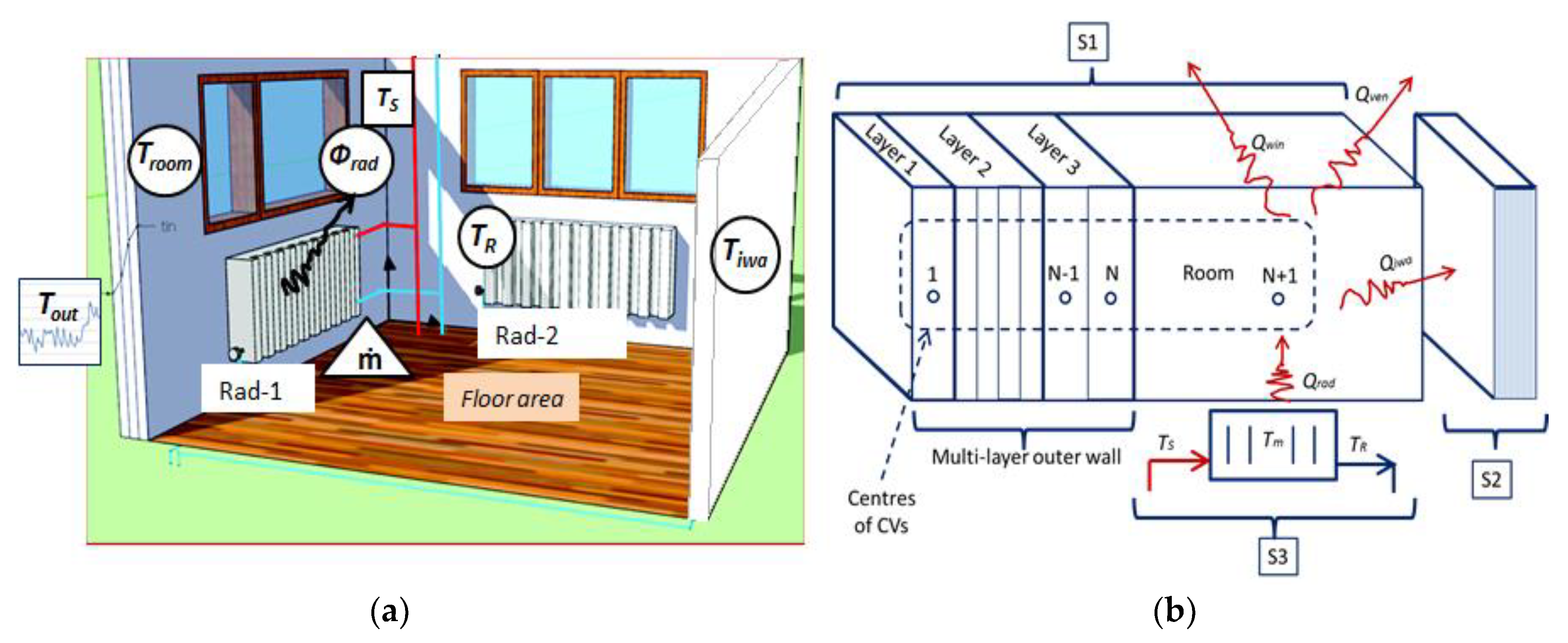
2.1. Modelling Assumptions

In this paper, the following assumptions are used to model the room heat balance. A room is presented with one computational control volume, which implies uniform room temperature. The radiator body thermal mass is added to the hot water thermal mass in Equation (3). It is assumed that all inner walls (upper, side, and floor walls) are represented with one thermal mass element. Inner wall conductivity is assumed to be very large, which implies that all surrounding inner walls are at the same temperature and are uniformly heated/cooled. At the opposite side of the inner walls, facing other rooms, an adiabatic boundary condition is assumed. This assumption implies that the surrounding rooms are heated as well as the one under observation.

2.2. Mathematical Model

The mathematical model is described with governing Equations (1)–(3) which reflect the behavior of the observed physical system. For multi-layer outer walls and room assembly, a modified transient heat conduction equation is used with additional heat sources and sinks, physically representing the transmission losses through windows, infiltration and ventilation losses, heat exchange with inner walls, and heat gains from the radiators. A separate thermal energy transport equation is solved for inner walls and finally the radiator equation contains transient, convective, and sink terms. The equations are strongly coupled, since the heat flux from radiators and from or to inner walls depend on the room temperature and vice versa. In the text which follows, the mathematical model with modelling assumptions is presented.

$$\frac{\partial }{\partial t}\underset{V}{\overset{}{{\displaystyle \int }}}\rho cTdV=\underset{S}{\overset{}{{\displaystyle \oint }}}k\nabla T·\mathrm{d}s+\langle -Q_{win}-Q_{iwa}-Q_{ven}+Q_{s,i}+Q_{rad}\rangle$$

(1)

$$\frac{\partial }{\partial t}\underset{V_{iwa}}{\overset{}{{\displaystyle \int }}}{\rho }_{iwa}{c}_{iwa} T_{iwa} dV=\underset{S^{\ast }}{\overset{}{{\displaystyle \int }}}{k}_{iwa} \nabla T_{iwa}· \mathrm{d}s+Q_{iwa}$$

(2)

$$\frac{\partial }{\partial t}\underset{V}{\overset{}{{\displaystyle \int }}}\left({\rho }_w{c}_w+{\rho }_{rb}{c}_{rb}\right)T_{m}dV+\underset{S}{\overset{}{{\displaystyle \oint }}}{\rho }_w{c}_w{T}_{w}v·\mathrm{d}s=-Q_{rad}$$

(3)

where $t$ is the time, $\rho$ is the density, $c$ is the specific heat, $T$ is temperature, $k\nabla T$ is the heat flux vector due to conduction heat transfer defined by Equation (4), ds is the surface vector perpendicular to the conductive heat flux vector, $Q_{win}$ are the windows transmission losses, $Q_{iwa}$ is the heat exchange between the room and inner walls, $Q_{ven}$ is ventilation/infiltration heat sink, $Q_{s,i}$ is the heat source from solar or/and internal gains, and $Q_{rad}$ is the heat flux exchanged between the radiator and observed room. Subscript iwa in Equation (2) denotes internal wall values, subscript w denotes water and subscript rb denote radiator body physical properties. Note that the terms in < > brackets in Equation (1) are valid for room only and they disappear in the part of the multi-layer walls where the pure transient heat conduction equation is solved.

The constitutive relationship between the heat flux and the temperature gradient for isotropic materials is given by Fourier’s law, Equation (4), and is already incorporated into transport Equation (1) within the first term at the right-hand side, as:

$$\mathit{q}=-k\nabla T$$

(4)

where q is the conductive heat flux, $k$ is the thermal conductivity, and $\nabla T$ is the temperature gradient.

Equation (2) describes the influence of the thermal capacity of the inner walls on heated rooms. These inner walls are at a different temperature from the room air and their large thermal capacity plays the role of a heat reservoir, source or sink, depending on the temperature gradient between the room and the internal walls. This is especially valid for intermittently heated buildings.

Since inner wall conductivity $k_{iwa}$ is assumed to be very large, the first term on the right-hand side of Equation (2) disappears, due to the fact that $\nabla T_{iwa}=0$. Equation (2) is coupled to Equation (1) via the convective heat transfer term $Q_{iwa}$ and this heat flux depends on the temperature difference between the inner wall and room temperature.

Equation (3) describes behavior of the radiators and $T_m$ represents the lumped temperature of the radiator, $T_w$ is the temperature of the flowing water at inlet and outlet of the radiator and $Q_{rad}$ is the heat sink or the heat flux from radiator towards the room air. Note that the heat flux from radiators is a heat source for the multi-layer outer walls and room assembly in Equation (1), while it is the heat sink in the radiator Equation (3). This means that Equations (1) and (3) are coupled via the term $Q_{rad}$.

2.3. Numerical Method

This paper proposes different approaches for solving the three coupled transport equations as proposed in the mathematical model section of the paper. Figure 1a represents the physical domain of the model room, while Figure 1b denotes the computational domain.

Variables in the rectangular boxes in Figure 1a are known values, such as $T_{out}$ as ambient temperature, $T_S$ as the radiator supply temperature, mass flow in the radiators $\dot{m}$ is given in a triangle, since its value has to be known and can be either calculated from the nominal conditions or measured values (see Section 3.3), the variables presented in circles, such as $T_{room}$ as room temperature, $Q_{rad}$ as radiator heat flux, $T_{iwa}$ as average internal wall temperature, and $T_R$ as the return temperature are unknown. At the Figure 1b, the calculation domain is presented with graphical symbols of the multi-layer wall and room assembly as domain 1 with solver 1 (S1), inner walls as domain 2 with solver 2 (S2), and the radiator as domain 3 with solver 3 (S3).

Figure 2 is the graphical representation of the coupling procedure in time. An explicit coupling procedure is adopted, which means that the room temperature is calculated based on the previous time step values of the room temperature (due to transient term discretization), inner wall temperature, and return temperature from the radiator, implicitly contained in the heat flux term $Q_{rad}$ in Equations (1) and (3). In what follows, the detailed discretization of different systems will be outlined.

For every transport equation the calculation details, boundary, and initial conditions are given, and at the end the overall solution algorithm is proposed.

2.3.1. Discretization of Multi-Layer Outer Walls and Room Assembly

For the multiple-layer outer wall and room assembly, the finite volume method (FVM) discretization principles are used. Discretization of space, time, and equations is implemented according to [17,18]. The space domain is divided into the finite number of control volumes (CVs), not necessarily of the same size, where the calculation points are located at the cell centers (collocated variable arrangement).

The Euler’s scheme of implicit integration in time is used, where the calculation time is divided into the final number of time intervals, not necessarily of the same duration. This scheme is of the first order of accuracy but is unconditionally stabile, irrespective of the time step size. Spatial discretization is performed assuming a linear variation of the dependent variable between adjacent calculation points (cell centers) and the integrals are calculated by using the mid-point rule, ensuring the second order accuracy. Diffusion coefficients are calculated at the cell-face centers as the weighting average between cell center values.

By applying adopted discretization principles, the resulting heat sources, Equations (5)–(8), in the thermal energy Equation (1) for the multi-layer wall and room assembly are calculated as:

$$Q_{win}=\underset{S_{win}}{\overset{}{{\displaystyle \int }}}{U}_{win}\left(T_{room}-T_{out}\right)dS\approx U_{win} \left(T_{room}-T_{out}\right) S_{win}$$

(5)

$$Q_{iwa}=\underset{S_{iwa}}{\overset{}{{\displaystyle \int }}}{\alpha }_{iwa}\left(T_{room}-T_{iwa}\right) dS \approx {\alpha }_{iwa} \left(T_{room}-T_{iwa}\right) S_{iwa}$$

(6)

$$Q_{ven}=\underset{V_{room}}{\overset{}{{\displaystyle \int }}}\frac{n_h\rho c\left(T_{room}-T_{out}\right)}{3600}dV\approx \frac{n_h}{3600}\rho c\left(T_{room}-T_{out}\right) V_{room}$$

(7)

$$Q_{rad}=\underset{A}{\overset{}{{\displaystyle \int }}}{q}_{rad} dA\approx Q_{rad}^N{\left(\frac{\Delta T_m}{\Delta T_m^N}\right)}^n$$

(8)

where $U_{win}$ is the heat transfer coefficient for windows, $T_{out}$ is the ambient temperature, $S_{win}$ is the area of windows, ${\alpha }_{iwa}$ is the heat transfer coefficient between the inner walls and room, $S_{iwa}$ is the area of inner walls in contact with the room, $n_h$ is the number of air changes per hour, $A$ is the surface of the radiator body, $Q_{rad}^N$ is the nominal heat flux of the radiator defined for nominal conditions, $\Delta T_m$ and $\Delta T_m^N$ are mean temperature difference between the radiator and the room for arbitrary and nominal conditions, respectively, and $n$ is the radiator exponent. Note that source terms given by Equations (5)–(8) are valid for the room only and they vanish in the multi-layer wall. The heat source due to solar and internal gains $Q_{s,i}$ is known and set in advance as a function of time.

Enumeration of control volumes is done from the outside layers towards the room (see Figure 1b), where the first CV is in contact with the environment and the last CV represents the room with index N + 1, where N is the sum of all CVs defined in the solid multi-layer wall. Note that number of CVs can be arbitrarily set for each layer of the wall.

In order to demonstrate the discretization practices, the balance according to Equation (1) will be written in discrete form for three neighboring CVs, given by Equations (9) and (10) and presented in Figure 3.

Figure 3 shows three neighboring cells with introduced compass notation where the observed cell, for which the balance will be given, is cell P, while the left-hand side or west cell is marked with letter W and the right-hand side or east cell is marked with letter E.

The discretized form of the transient term in Equation (1) becomes:

$$\frac{\partial }{\partial t}\underset{V}{\overset{}{{\displaystyle \int }}}\rho cTdV\approx \frac{\delta V_P}{\delta t}\left[{\left(\rho cT\right)}_P-{\left(\rho cT\right)}_P^{m-1}\right]$$

(9)

where $\delta V_P$ is the volume of the CV with center P, $\delta t$ is the time step size, subscript P denotes values from the cell center P, while the exponent $m-1$ denotes values from the previous time step.

The discretized form of the diffusion flux in Equation (1) becomes:

$$\underset{S}{\overset{}{{\displaystyle \oint }}}k\nabla T·\mathrm{d}s\approx \frac{k_e}{{\delta }_{PE}}\left(T_E-T_P\right) S_e-\frac{k_w}{{\delta }_{WP}}\left(T_P-T_W\right) S_w$$

(10)

where $k_e$ and $k_w$ are the conductivities calculated at the cell face surfaces e (between cell E and P) and w (between cells W and P), respectively, ${\delta }_{PE}$ and ${\delta }_{WP}$ are distances between cell centers P and E and W and P, respectively, and $T_P$, $T_W$, and $T_E$ are values of the temperatures in cell centers P, W, and E, respectively. Note that the first term on the right-hand side of Equation (10) is the heat flux at the east cell face surface, while the second term represents the heat flux at the west cell face surface. The cell face value of conductivity, Equation (11), for example at cell face e, is according to [18] and is calculated as:

$$\frac{k_e}{{\delta }_{PE}}=\frac{1}{\frac{{\delta }_{Pe}}{k_P}+\frac{{\delta }_{eE}}{k_E}}$$

(11)

where ${\delta }_{Pe}$ is the distance between cell center P and cell face e, ${\delta }_{eE}$ is the distance between cell face e and cell center E (see Figure 3), while $k_P$ and $k_E$ are the conductivities in cell centers P and E, respectively. Note that usual approach is to find the linear interpolation of conductivities at the cell faces, which, in the case of large differences of conductivities in CVs P and E, introduces calculation error. By using the current approach, the diffusive coefficient at the cell face is calculated correctly.

A special treatment is necessary for the first and last cell in the multi-layer wall, which is given by Equations (12) and (13). If point P is the first cell which neighbors the ambient environment (Figure 4 left side), then the west cell face conductivity is calculated as:

$$\frac{k_{w1}}{{\delta }_{B1}}=\frac{1}{\frac{1}{{\alpha }_{out}}+\frac{{\delta }_{B1}}{k_1}}$$

(12)

where ${\alpha }_{out}$ is the heat transfer coefficient from the outside wall to environment. In the case that point P is neighboring the room (Figure 4 right), the cell face conductivity is calculated according to:

$$\frac{k_e}{{\delta }_{Ne}}=\frac{1}{\frac{{\delta }_{Ne}}{k_N}+\frac{1}{{\alpha }_{in}}}$$

(13)

where ${\alpha }_{in}$ is the heat transfer coefficient from the room to the outside-facing wall.

The final form of the discretized Equation (14) is written in the form:

$$a_P{T}_P-{\displaystyle \sum }_j{a}_j{T}_j=b_P$$

(14)

where index j = {E,W} denote position of the CV according to compass notation, $a_P$ is the central coefficient with values near $T_P$, $a_j$ are the neighbour coefficients new temperature values $T_j$, and the right hand side is the source term $b_P$.

For exemplary cell P given in Figure 3, the values of the neighboring and central coefficients as well as the source terms are given in Equations (15)–(17) as:

$$a_E=\frac{S_e}{\frac{{\delta }_{Pe}}{k_P}+\frac{{\delta }_{eE}}{k_E}}\hspace{1em}{a}_W=\frac{S_w}{\frac{{\delta }_{wW}}{k_W}+\frac{{\delta }_{wP}}{k_P}}$$

(15)

$$a_P=\frac{\delta V_P{\rho }_P{c}_P}{\delta t}+a_E+a_W+\langle U_{win}{S}_{win}+{\alpha }_{iwa}{S}_{iwa}+\frac{n_h}{3600}\delta V_P{\rho }_P{c}_P\rangle$$

(16)

$$b_P=\frac{\delta V_P{\rho }_P{c}_P}{\delta t}{T}_P^{m-1}+\langle U_{win}{S}_{win}{T}_{out}+{\alpha }_{iwa}{S}_{iwa}{T}_{iwa}+\frac{n_h}{3600}\delta V_P{\rho }_P{c}_P{T}_{out}+Q_{s,i}+Q_{rad}^{\ast }\rangle$$

(17)

If for all CVs within the solution domain of multi-layer walls and room assembly one writes coefficient and source terms, now by following enumeration given in Figure 1b, a system of N + 1 linear equations will be obtained. Note that the part of the heat flux in expressions (5)–(7), containing the room temperature are transferred to the central coefficient in Equation (16). The remaining parts of these fluxes are part of the source terms in Equation (17) and contain known values such as ambient temperatures $T_{out}$ and inner wall temperature $T_{iwa}$ (explicit coupling).

The system of equations can also be written in the vector format, given by Equation (18) as:

$$A x=b$$

(18)

where A is the coefficient matrix, x is the vector of the dependent variable—in our case temperature— and b is the vector of the source terms. By preserving introduced compass notation, Equation (18) can be also written in a matrix form, Equation (19), as:

$$\left(\begin{array}{cccccc}{a}_{P1}& a_{E1}& 0& 0& 0& 0\\ a_{W2}& a_{P2}& a_{E2}& 0& 0& 0\\ 0& a_{W3}& a_{P3}& a_{E3}& 0& 0\\ \cdots & \cdots & \cdots & \cdots & \cdots & \cdots \\ 0& 0& 0& a_{W\left(N\right)}& a_{P\left(N\right)}& a_{E\left(N\right)}\\ 0& 0& 0& 0& a_{W\left(N+1\right)}& a_{P\left(N+1\right)}\end{array}\right)·\left(\begin{array}{c}{T}_1\\ T_2\\ T_3\\ \cdots \\ T_N\\ T_{N+1}\end{array}\right)=\left(\begin{array}{c}{b}_{P1}\\ b_{P2}\\ b_{P3}\\ \cdots \\ b_{P\left(N\right)}\\ b_{P\left(N+1\right)}\end{array}\right)$$

(19)

where $a_{Pi}$ are the central coefficients or previously declared as $a_P$, for example, given in Figure 3 and Equation (16), where i is the counter of CVs and goes from I = 1 to N + 1 CVs, while N + 1 represents the index of the room. Note that the matrix is tridiagonal and all source terms $b_{Pi}$ are known, since the explicit coupling procedure is adopted. Note that the heat flux from the radiators $Q_{rad}^{\ast }$ featuring in Equation (17) is calculated based on the $T_{room}$ value taken from the previous time step.

It means that the system given in Equation (19) can be solved by a direct algorithm known as the three diagonal matrix algorithm (TDMA) or the Thomas algorithm. All temperature values are obtained in two passes. First the system, Equation (19) is written in the form of Equation (20) as:

$$a_{Wi}{T}_{i-1}+a_{Pi}{T}_i+a_{Ei}{T}_{i+1}=b_i,\hspace{1em}\left(i=1, 2, \dots , N+1\right)$$

(20)

TDMA uses Gaussian elimination to put the system in upper triangular form by computing the new diagonal coefficients $a_{Pi}$ and the new right-hand side vector components $b_i$ given by Equation (21), while the unknown temperatures are obtained from the backward substitution as given by Equation (22):

$$a_{Pi}=a_{Pi}-\frac{a_{Wi}}{a_{P\left(i-1\right)}}{a}_{E\left(i-1\right)},\hspace{1em}{b}_i=b_i-\frac{a_{Wi}}{a_{P\left(i-1\right)}}{b}_{\left(i-1\right)},\hspace{1em}\left(i=2,3, \dots , N+1\right)$$

(21)

where the equal sign means that the value is replaced by.

$$T_{N+1}=\frac{b_{N+1}}{a_{P\left(N+1\right)}} ,\hspace{1em}{T}_i=\frac{b_i-a_{Ei}{T}_{i+1}}{a_{Pi}} ,\hspace{1em}\left(i=N,N-1, \dots ,1\right)$$

(22)

The original set of integral-differential equations is transformed into algebraic equations by the discretization practices described above. Linearization of the source terms is implemented by implicit treatment of heat sources/sinks as part of the coefficient matrix, which together with explicit coupling of equations results in a tridiagonal system of equations solved by TDMA.

2.3.2. Final Form of the Transport Equation for Inner Walls

The assumption of modelling all inner walls with a unit thermal mass element implies the use of one computational cell for inner walls. In this case, the temporal Euler’s explicit scheme is used, while the spatial discretization does not make sense. The algebraic equation which is solved for inner walls, Equation (23), has the final form:

$$T_{iwa}=T_{iwa}^{old}+\frac{{\alpha }_{iwa}{S}_{iwa}}{\frac{m_{iwa}{c}_{iwa}}{\delta t}}\left(T_{room}^{\ast }-T_{iwa}^{old}\right)$$

(23)

where $m_{iwa}$ is the mass of the inner walls as a product of the inner wall density and volume, superscript $old$ means that the values are taken from the previous time step and $T_{room}^{\ast }$ is the last available room temperature, taken from the previous time step. It can be noted that no special solver is needed for the transport equation of the inner walls, since it can be solved explicitly, bearing in mind that all variables at the right-hand side of Equation (23) are already known.

2.3.3. Final Form of Transport Equation for Radiators

In order to make the equation valid for radiators, the unknown variables need to be declared for Equation (3). The lumped radiator temperature $T_m$ is in this work calculated as the arithmetic average according to Equation (24):

$$T_m=\frac{T_S+T_R}{2}$$

(24)

where $T_S$ is the radiator water supply temperature and $T_R$ is the water return temperature. Note that in the current study, a simple, one-zone heating system is envisaged with weather compensated control, which means that the supply temperature in the radiator is almost the same as the heating system’s supply temperature (no mixing valve in the supply nor the return pipe and negligible thermal losses).

Temperature differences $\Delta T_m$ and $\Delta T_m^N$ at the right-hand side of Equation (8) are calculated by treating the radiator as a heat exchanger. The consequence is that the log mean temperature difference (LMTD) is used and $\Delta T_m$ is calculated by Equation (25):

$$\Delta T_m=\frac{T_S-T_R}{ln\frac{T_s-T_{room}}{T_R-T_{room}}}$$

(25)

where this expression is valid for arbitrary conditions as well as for the nominal radiator conditions.

The governing equation for the radiator (3) is discretized by assuming the mid-point rule for calculation of integrals and by using Euler implicit time integration. In this case, the domain of the radiator body contains only one computational cell and is not discretized into a finite number of calculation points. In the transient calculation of heat transfer from radiators to the surrounding air, the bisection method was used. Equation (26) has been numerically solved, where the $U{A}^N$ value is defined by Equation (27):

$$\frac{\left(m_{rb}{c}_{rb}+V_w{\rho }_w{c}_w\right)}{\delta t}\left[\left(\frac{T_S+T_R}{2}\right)-T_m^{old}\right]-\dot{m}{c}_w\left(T_S-T_R\right)=-U{A}^N{\left[\frac{T_S-T_R}{ln\left(\frac{T_S-T_{room}^{\ast }}{T_R-T_{room}^{\ast }}\right)}\right]}^n$$

(26)

where

$$U{A}^N=\frac{Q_{rad}^N}{{\left(\Delta t_m^N\right)}^n}$$

(27)

is the radiator constant which is related to the nominal conditions of the radiator, its power $Q_{rad}^N$, and $\Delta t_m^N$ the difference between the average radiator surface temperature and the room temperature in nominal conditions and calculated according to (25). Note that constant $U{A}^N$ represents the product of the overall heat transfer coefficient and the area of radiator and physically implies the constant U value of the radiator over different temperature regimes and/or mass flows in the radiator.

An additional variable which needs to be determined is mass flux $\dot{m}$ appearing in Equation (26). Mass flux can be calculated for the nominal temperature regime of the radiator, which is given by producers. However, in most practical situations, the real mass flow in radiator differs from the nominal mass flow. In cases where the measurements of the room temperature exists, where supply and return temperatures are known, the mass flux can be estimated.

Equation (26) is solved by the halving interval method (bisection method) iteratively for $T_R$ as a dependent variable within an initially prescribed interval:

$$T_{room}\le T_R\le T_S$$

The presented mathematical model and calculation procedure implies known supply temperature, which is always the case when weather compensated control is used. Equation (26) is iteratively solved until the convergence criteria is reached (i.e., less than $1\times {10}^{-4}$).

2.4. Solution Algorithm

The solution procedure is executed as follows:

• Data for domain of multi-layer walls and room assembly are defined
  • Dimensions of the room and surface of outer wall are prescribed,
  • Dimensions of windows are defined,
  • Arbitrary number of layers in the multi-layer wall are prescribed with their physical properties and an arbitrary number of control volumes is assigned for each layer,
• Data for inner walls are defined
  • Heat capacity is prescribed with mass of all inner walls and their specific heat,
  • Heat transfer coefficient and surface from inner walls to room air is defined,
• Radiator parameters are defined
  • Nominal radiator capacity,
  • Nominal regime as nominal supply, return, and room temperature,
  • Physical properties of mass and specific heat of the radiator body, including the content of the water in the radiator is prescribed,
  • Relevant mass flow is defined, either taken from nominal conditions or from the measurements (where available),
• Initial and boundary conditions are given for all equations;
  • Initial temperature profile in the outer wall (constant or arbitrary), initial room temperature, initial inner wall temperature, initial hot water supply temperature, and initial lumped temperature of radiators (equal or larger than room temperature) are prescribed,
  • Boundary conditions are applied by assuming known, variable, or fixed outside temperature and known hot water supply temperature (note that in weather compensated heating control both values are known),
• The system of Equations (19) is solved by using the TDMA solver and by assuming the known radiator heat flux and the inner wall heat flux from the previous time step, resulting in the new room temperature value,
• Equation (23) for inner walls is solved, resulting in a new inner wall temperature
• Equation (26) for radiators is solved iteratively to get the new return temperature by using the current values of supply temperature and last available room temperature value from the previous time step,
• Steps 5 to 7 are repeated until the final time step is reached.

3. Results

In this section, the developed methodology is verified and validated on three characteristic test cases. Validation cases are carefully selected in order to test the validity and correctness of all described features. The setups of these cases are explained in detail and the expected results are outlined. The verification process is completed when the results of the calculations correspond to the expected values, which can be obtained analytically. The main features of the selected cases are described below, while the detailed setup and parameters for calculations are outlined in the following subsections:

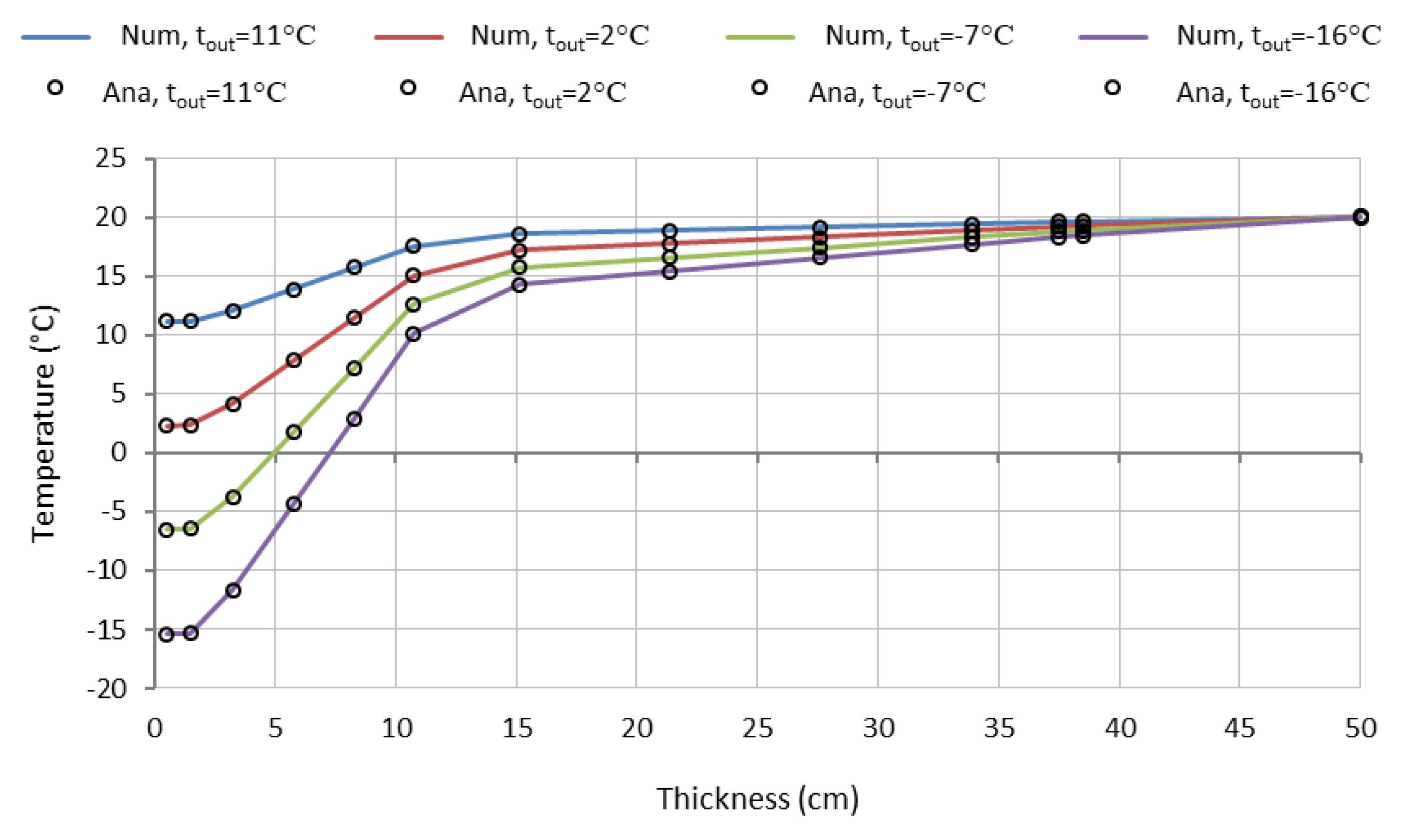
• Case 1 presents the test case in which several features of the tool are tested. Calculations are run transiently with constant outside temperature, leading to the solution of coupled equations to the steady-state result. In this case, the thermal inertia of the inner walls is assumed to be reasonably low. Different initial temperatures are given for the outer wall, room, and inner walls. When the steady-state is reached, the results of calculation are compared to the values of expected room and inner wall temperatures (should be equal) and expected radiator heat flux, which should compensate for heat losses of the room to the environment. Also, the temperature profiles in the multi-layer outer wall are compared against the analytical solutions for four characteristic and different values of outside temperatures, each run as separate calculations.
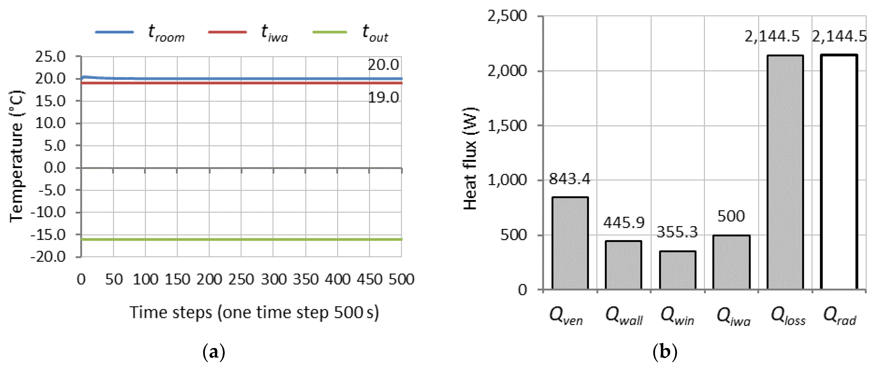
• Case 2 demonstrates a case where the thermal inertia of inner walls is huge, which causes the inner wall temperature to remain constant during the calculations, introducing an additional heat loss to the room. Calculation is run transiently and the expected values—prescribed room temperature and constant inner walls’ temperature—are analyzed when the steady-state is reached. The simulation is run for design conditions in terms of outside and set room temperatures.
• Case 3 is designed to test the interaction between the heat flux from radiators towards the room and the heat flux between the room and the environment. For this purpose, the thermal inertia of the outer, inner walls, and a radiator is neglected, providing zero influence of the transient terms in Equations (1)–(3). Variable outside temperature is prescribed in time and the calculation is run transiently, formally providing the steady-state solutions for every time step due to the mentioned assumptions.

The calculation domain is presented in symbolic form in Figure 5, where all elements used in the calculations are shown. The geometry of the room, composition of multi-layer outside walls, heat transfer coefficients, size of windows, and infiltration rate are identical for cases 1, 2, and 3. Note that the solar and internal gains are neglected ($Q_{s,i}=0$) in all test cases since they are strongly transient in nature and because their implementation is straightforward.

The test room consists of two outer walls with the same structure, each made of 4 layers (materials). There is one window, one radiator, and all inner walls are represented by one block.

Table 1. Geometry and characteristic parameters for test cases 1, 2, and 3.

Test Case	Room Size (B/H/W) in m	${\mathit{S}}_{\mathit{w}\mathit{i}\mathit{n}} {\mathbf{m}}^2$	${\mathit{U}}_{\mathit{w}\mathit{i}\mathit{n}} \mathbf{W}/{\mathbf{m}}^2\mathbf{K}$	${\mathit{n}}_{\mathit{h}} {\mathbf{h}}^{-1}$	${\mathit{S}}_{\mathit{w}\mathit{a}\mathit{l}\mathit{l}} {\mathbf{m}}^2$	HT Coeff. W/m2K		Design Temp. °C
						αin	αout	${\mathit{t}}_{\mathit{r}\mathit{o}\mathit{o}\mathit{m}}^{\mathit{N}}$	${\mathit{t}}_{\mathit{o}\mathit{u}\mathit{t}}^{\mathit{N}}$
Cases 1, 2, 3	5/8/3.5	7.05	1.4	0.5	38.45	20	8	20	−16

presents the room size and other characteristic values relevant for step 1 in the setup procedure described in the previous section. In the last two columns, the outside and room temperatures are given, which are relevant for calculation of nominal losses of the room and for sizing the installed power of the radiator.

Two outside walls are defined with 4 layers, as given in

Table 2. Thermo-physical properties of outer walls.

Layer	Material	Thickness, m	Thermal Conductivity, W/mK	Specific Heat, J/kgK	Density, kg/m3
1	Cement mortar	0.02	1.40	1000	1800
2	EPS	0.10	0.04	1450	20
3	Hollow brick	0.25	0.64	900	1600
4	Lime mortar	0.02	0.81	1000	1500

, with different thicknesses and corresponding thermo-physical properties: thermal conductivity, specific heat, and density. Based on the data given in Table 1 and Table 2, it is possible to calculate the overall U value of the multi-layer wall and then to calculate the nominal heat losses of the observed room as:

$$Q_{loss}^N=\left(U_{wall}{S}_{wall}+U_{win}{S}_{win}+\frac{n_h\rho cV}{3600}\right) \left(t_{room}^N-t_{out}^N\right)+Q_{iwa}^{\ast }$$

(28)

where $Q_{loss}^N$ are the total heat losses in nominal conditions, $U_{wall}{S}_{wall}$ is the product of U value of wall and area of wall representing the coefficient of heat transmission through walls, $U_{win}{S}_{win}$ is the product of the U value of window and area of window representing the coefficient of transmission losses through the windows, and the last term in brackets represents the coefficient of infiltration-ventilation losses, where $n_h$ is the number of air changes per hour, $\rho c$ is the product of air density and specific heat, and $V$ is the room volume. The last term on the right-hand side of Equation (28), $Q_{iwa}^{\ast }$, is the heat flux between the room and inner wall and will be discussed for all cases.

Table 3. Physical properties of inner walls and radiator data for all test cases.

Test Cases	Inner Wall Properties				Radiator Parameters
	${\mathit{m}}_{\mathit{i}\mathit{w}\mathit{a}}$ kg	${\mathit{c}}_{\mathit{i}\mathit{w}\mathit{a}}$ J/kgK	${\mathit{S}}_{\mathit{i}\mathit{w}\mathit{a}} {\mathbf{m}}^2$	${\mathit{\alpha }}_{\mathit{i}\mathit{w}\mathit{a}} \mathbf{W}/{\mathbf{m}}^2\mathbf{K}$	${\mathit{Q}}_{\mathit{r}\mathit{a}\mathit{d}, }^{\mathit{N}}\mathbf{W}$ 90/70/20	${\mathit{Q}}_{\mathit{r}\mathit{a}\mathit{d}}, \mathbf{W}$ 80/60/20	$\dot{\mathit{m}}$ kg/s	Supply Temp.
Case 1	100	1400	100	5	2084.3	1644.5	0.019	Heat curve
Case 2	$1\times {10}^6$	$1\times {10}^6$			2718.1	2144.5	0.026
Case 3	0	0	0	0	2084.3	1644.5	0.019

contains the relevant properties for the inner wall and radiator data for all test cases. It can be seen that for Case 2, the thermal capacity of the inner wall (product of mass and specific heat) is set as a very large value, while it is zero for Case 3. In contrast, for Case 1, the thermal capacity of the inner wall is defined as a relatively small value. These facts are discussed in more detail in subsections which describe the specific setup for each test case. The last column in Table 3 represents the supply temperature of the heating system, which is, in this paper, taken as the water temperature entering the radiator (no heat losses are envisaged between the boiler and radiator).

For cases 1 and 2, a constant outside temperature is prescribed, which results in constant water supply temperature based on heat curve values. If one links this assumption to reality, this would mean that the system is working according to weather compensated control, by which the heat flux from the radiators is controlled via water supply temperature. The mass flow for all test cases remains constant during the calculations (values are given in Table 3), by which it is assumed that neither variable speed drive pumps nor thermostatic valves exist in the system.

In terms of the boundary conditions, for all test cases, only the outside temperature is prescribed, while the supply water temperature is calculated according to the heat curve parameters. The radiator mass flow is calculated according to the work conditions of the heating system, while all other variables remain unknown, such as the temperatures in the CV centers in multi-layer wall (in all calculation taken as 12 CVs), room and inner wall temperatures (1 + 1 unknown value), the heat flux from the radiator, and water return temperature (1 + 1 unknown value).

3.1. Validation Case 1—Low Thermal Inertia of Inner Walls

For this case, a radiator is chosen so that its heat flux in working conditions exactly compensates the total heat losses of the room in nominal conditions (for design temperatures). For the sake of radiator testing, producer data corresponding to a nominal radiator regime 90/70/20 °C is chosen, while it is supposed that the heating system works according to regime of 80/60/20 °C. Note that the first number denotes the water supply temperature, the second number is the water return temperature, and the third number is a room temperature. The mass flow in the radiator is calculated based on the nominal room heat loss in design conditions ($Q_{loss}^N=1644.5 \mathrm{W}$) and according to the working regime of the heating system.

For testing purposes, four different outside temperature values are used, run as four different calculations. Based on Equation (1), the value of outside temperature is calculated in order to get the room heat losses as a percentage of nominal room heat losses. The adopted values are 25%, 50%, 75%, and 100% based on nominal room heat losses and the corresponding prescribed outside temperatures are 11 °C, 2 °C, −7 °C, and −16 °C, respectively.

Since weather compensated control is used, for every given outside temperature, a corresponding water supply temperature is calculated according to the heat curve parameters. The values are given in the second column of

Table 4. Boundary conditions, supply water temperature, and losses.

Outside Temperature tout (°C)	Water Supply Temp. tS (°C)	Heat Losses Qloss (W)	Qloss/QlossN (%)
−16	80.0	1644.5	100
−7	67.6	1233.4	75
2	54.3	822.3	50
11	39.7	411.1	25

.

Initial conditions for all outside temperatures are the same and are given as:

$$t_w^{in}\left(i\right)=19 °\mathrm{C} ; t_{iwa}^{in}=19 °\mathrm{C} ; t_{room}^{in}=15 °\mathrm{C}$$

(29)

where $t_w^{in}\left(i\right)$ are the initial temperatures in the multi-layer outside wall, where i = 1 to 12 (for 12 CVs), $t_{iwa}^{in}$ is the initial temeprature of the inner wall, and $t_{room}^{in}$ is the initial room temperature. Since the outside temperature is fixed as a constant value, the problem has a unique solution, irrespective of the prescribed initial conditions. The influence of the transient terms in the equations exists at the beginning of the calculations and decreases over time until it completely vanishes when a steady-state is reached.

Validation of the model also requires the validation of the heat balance between the room and inner wall. In this case, since the small thermal capacity of the inner wall is assumed, it is expected that the inner wall temperature will reach the room temperature at the steady-state.

It is assumed that the steady-state condition is reached when the difference between the heat fluxes, measured at the exterior and interior surfaces of the multi-layer outer wall is less than 0.5%. Figure 6a shows the overlapping room and inner wall temperature profiles in time and the radiator heat fluxes (Figure 6b), both for four different values of outside temperature. One can confirm that in all cases $t_{iwa}=t_{room}=20 °\mathrm{C}$. In Figure 6b, beside the temporal variation of radiator heat fluxes, the steady-state heat flux values are given as data labels. It can be seen that for all four cases, the radiator heat fluxes are almost the same as the calculated room heat losses (Table 4). The largest relative error between the calculated radiator flux value and the prescribed room heat loss value is 0.02%, which is practically negligible. This value could be further decreased by forcing stricter steady-state criteria (less than 0.5% difference in heat fluxes at exterior and interior surface).

Figure 7 shows the comparison between analytical results and the results of calculation for four different values of outside temperature. It can be seen that perfect matching is achieved, proving that all the tested features passed the verification process.

3.2. Validation Case 2—High Thermal Inertia of Inner Walls

In this case, the influence of the extremely high thermal inertia of the inner walls is considered, as shown in Table 3. The size of the room and the composition of the outer walls remain the same as in test Case 1, including identical initial conditions defined by expression (29). The only difference is the increased nominal power of the radiator, since it has to cover additional heat flux losses to the inner walls, even when the steady-state is reached.

Based on the values for ${\alpha }_{iwa}$ and $S_{iwa}$ given in Table 3, the additional heat flux in this case is $Q_{iwa}^{\ast }=500 \mathrm{W}$ and this is exactly the additional required power for a radiator in a heating system regime 80/60/20 °C. In this case, the calculation is run as transient with constant prescribed outside temperature corresponding to the design conditions, $t_{out}=-16 °\mathrm{C}$.

The results of the calculation proved that the expected values are obtained when the steady-state condition is reached (Figure 8). In Figure 8a, the outside, room, and inner wall temperatures are given as a function of time (x axis), while in Figure 8b, the components of the total heat flux losses (grey data bars) and the radiator flux (white data bar) are given. One can note that in this case, even though the temperature difference between the room and inner wall is 1 °C, the contribution of the inner wall heat flux is more than 23% in total heat flux/losses. The calculation results confirmed the expected results and the case is validated.

3.3. Validation Case 3—No Thermal Inertia of Inner and Outer Walls

This case is designed to validate the use of coupled equations between a multi-layer outer wall and the room assembly at one side and the radiator equation at the other side. For arbitrary variation of the outside temperature, the supply water temperature is determined according to the heat curve parameters and set as a boundary condition for radiator equation. In this case, the size of the room remains the same, while the non-existing thermal inertia of the outer walls is defined by setting the specific heat and density to zero for all four layers of the outer wall. Inner wall heat transfer is neglected by setting $S_{iwa}=0$ (see Table 3), and radiator thermal inertia is also neglected by assuming near zero mass of the radiator body and near zero water content in the radiator.

As a result of all assumptions, the heat losses for the prescribed room temperature of 20 °C can be calculated by using Equation (30) as:

$$Q_{loss}\left(\tau \right)=\left(U_{wall}{S}_{wall}+U_{win}{S}_{win}+\frac{n_h\rho cV}{3600}\right) \left[20-t_{out}\left(\tau \right)\right]$$

(30)

where $Q_{loss}\left(\tau \right)$ is the heat loss as a function of the time $\tau$ and $t_{out}\left(\tau \right)$ is the outside temperature variation given as function of time.

One can see that the influences of the transient terms are completely neglected by the derivation of expression (30). The expected results of the calculations should keep the constant room temperature of $t_{room}\left(\tau \right)=20 °\mathrm{C}$ for any $\tau$. Also, the radiator heat flux should be equal to the $Q_{loss}\left(\tau \right)$ for any $\tau$.

Figure 9a shows the variation of the outside temperature and the calculated room temperature, which is maintained at the constant and set value of $20 °\mathrm{C}$. Variation of room heat losses (circles) calculated by using expression (30) are compared to calculated radiator flux values, presented by a full line in Figure 9b. It can be seen that the expected results are achieved and that the Temperature Solver satisfied all tests.

The verification and validation process was completed and the conclusion is that the proposed and implemented methodology provides correct results.

4. Conclusions

A mathematical model and solution algorithm have been developed for analysis of single rooms in intermittently heated buildings, considering transient effects. The methodology introduces the additional influence of the thermal capacity of inner walls, which is often neglected in calculations. The optimal start time of the heating system is influenced by the temperature of the inner walls and can affect energy consumption of the overall building. At the moment, there are no simple guidelines for optimal starting of the system in order to minimize energy consumption while providing thermal comfort. This paper is one step forward in this direction, which, combined with measurements of pilot buildings and rooms, can support engineers to find the optimal solution.

The second major intention of this paper is to demystify transport energy equations and present them in a simple to solve form. This is especially designed for practitioners whose mathematical skills are lacking, regarding the current needs in the Heating, Ventilation and Air-Conditioning (HVAC) business. The developed methodology was rigorously tested and validated on cases for which analytical solutions exist. The developed methodology is currently being tested versus measurements in real buildings. The preliminary comparisons of calculated and measured values show promising results which will be the subject of a separate publication. Further development and application will cover an extension of the methodology for calculation of the optimal heat flux from radiators to maintain the desired room temperature, as well as including modeling of thermostatic valves mounted on radiators.

References

1. Directive 2010/31/EU of the European Parliament and of the Council of 19 May 2010 on the energy performance of buildings (EPBD). Off. J. Eur. Union 2010, 153, 13–35.
2. Directive 2012/27/EU on energy efficiency (EED) of the European Parliament and of the Council of 25 October 2012. Off. J. Eur. Union 2012, 315, 1–56.
3. Blazevic, R. Advanced Modeling and Dynamic Simulation of the Heating System with the Simultaneous Application of Modelica and the Final Volume Method. Ph.D. Thesis, University of Sarajevo, Sarajevo, Bosnia and Herzegovina, 2018. (In Bosnian). [Google Scholar]
4. Kensby, J.; Trüschel, A.; Dalenbäck, J.O. Potential of residential buildings as thermal energy storage in district heating systems—Results from a pilot test. Appl. Energy 2015, 137, 773–781. [Google Scholar] [CrossRef]
5. Romanchenko, D.; Kensby, J.; Odenberger, M.; Johnsson, F. Thermal energy storage in district heating: Centralized storage vs. storage in thermal inertia of buildings. Energy Convers. Manag. 2018, 162, 26–38. [Google Scholar] [CrossRef]
6. Crawley, D.B.; Lawrie, L.K.; Winkelmann, F.C.; Buhl, W.F.; Huang, Y.J.; Pedersen, C.O.; Strand, R.K.; Liesen, R.J.; Fisher, D.E.; Witte, M.J.; et al. EnergyPlus: Creating a new generation building energy simulation program. Energy Build. 2001, 33, 443–457. [Google Scholar] [CrossRef]
7. Delcroix, B.; Kummert, M.; Daoud, A.; Hiller, M.D. Conduction Transfer functions in TRNSYS multi-zone building: Current implementation, limitations and possible improvements. In Proceedings of the Fifth National Conference of International Building Performance Simulation Association, Madison, WI, USA, 1–3 August 2012. [Google Scholar]
8. Wetter, M. Multizone building model for thermal building simulation in Modelica. In Proceedings of the 5th International Modelica Conference, Vienna, Austria, 4–5 September 2006; Kral, C., Haumer, A., Eds.; Modelica Association and Arsenal Research: Vienna, Austria, 2006; Volume 2, pp. 517–526. [Google Scholar]
9. Wetter, M.; Zuo, W.; Nouidui, T.S. Modeling of heat transfer in rooms in the Modelica “Buildings” Library. In Proceedings of the Building Simulation 2011: 12th Conference of International Building Performance Simulation Association, Sydney, Australia, 14–16 November 2011. [Google Scholar]
10. Nouidui, T.S.; Phalak, K.; Zuo, W.; Wetter, M. Validation and Application of the Room Model of the Modelica Buildings Library. In Proceedings of the 9th International Modelica Conference 2012, Munich, Germany, 3–5 September 2012; Simulation Research Group, Building Technology and Urban Systems Department Environmental Energy Technologies Division, Lawrence Berkeley National Laboratory: Berkeley, CA, USA, 2012. [Google Scholar]
11. Felgner, F.; Cladera, R.; Merz, R.; Litz, L. Modelling Thermal Building Dynamics with Modelica; Kaiserslautern University of Technology, Institute of Automatic Control: Kaiserslautern, Germany, 2003. [Google Scholar]
12. Wetter, M.; Haugstetter, C. Modelica versus TRNSYS—A Comparison between an Equation-Based and a Procedural Modeling Language for Building Energy Simulation; United Technologies Research Center: East Hartford, CT, USA, 2006. [Google Scholar]
13. Sodja, A.; Zupančič, B. Modelling thermal processes in buildings using an object-oriented approach and Modelica. Simul. Model. Pract. Theory 2009, 17, 1143–1159. [Google Scholar] [CrossRef]
14. Skruch, P. A Thermal Model of the Building for the Design of Temperature Control Algorithms. Automatyka/Automatics 2014, 18, 9–21. [Google Scholar] [CrossRef]
15. Verbeke, S.; Verhaert, I.; Audenaert, A. Thermal inertia in dwellings: Adapting thermostat schedules in relation to the building thermal mass. In Proceedings of the REHVA Annual Meeting Conference Low Carbon Technologies in HVAC, Brussels, Belgium, 23 April 2018. [Google Scholar]
16. Byrne, A.; Byrne, G.; Davies, A.; Robinson, A.J. Transient and quasi-steady thermal behaviour of a building envelope due to retrofitted cavity wall and ceiling insulation. Energy Build. 2013, 61, 356–365. [Google Scholar] [CrossRef] [Green Version]
17. Demirdzic, I.; Muzaferija, S.; Peric, M. Advances in computation of heat, fluid flow and solid body deformation using finite volume approaches. Adv. Numer. Heat Transf. 1997, 2, 59–96. [Google Scholar]
18. Teskeredzic, A.; Demirdzic, I.; Muzaferija, S. Numerical method for calculation of complete casting process—Part I, Theory. Numer. Heat Transf. Part B 2015, 68, 295–316. [Google Scholar] [CrossRef]
Figure 1. (a) Physical domain of the model room; (b) Calculation domain.
Buildings 08 00163 g001
Figure 2. Graphical representation of the explicit coupling procedure.
Buildings 08 00163 g002
Figure 3. Three neighboring CVs with compass notation (P—central cell center, W—west cell center, E—east cell center).
Buildings 08 00163 g003
Figure 4. Special calculation of coefficients and source terms for marked surfaces (exposed to ambient—left hand side and at interface outer wall and room—right hand side).
Buildings 08 00163 g004
Figure 5. Geometry for test cases 1, 2, and 3.
Buildings 08 00163 g005
Figure 6. (a) Room temperature values in time; (b) Radiator heat flux Q r a d , for four different values of outside temperature.
Buildings 08 00163 g006
Figure 7. Comparison of the numerical calculation results with the analytical results for different values of ambient temperature.
Buildings 08 00163 g007
Figure 8. (a) Outside, room, and inner wall temperature; (b) Ventilation, transmission wall, transmission windows, internal wall flux, total losses (grey data bars), and radiator flux (white data bar).
Buildings 08 00163 g008
Figure 9. (a) Room and variable outside temperature; (b) Comparison of radiator flux versus total heat losses.
Buildings 08 00163 g009