SSI on the Dynamic Behaviour of a Historical Masonry Building: Experimental versus Numerical Results

Abstract

A reliable procedure to identify the dynamic behaviour of existing masonry buildings is described in the paper, referring to a representative case study: a historical masonry palace located in Benevento (Italy). Since the building has been equipped with a permanent dynamic monitoring system by the Department of Civil Protection, some of the recorded data, acquired in various operating conditions, have been analysed with basic instruments of the Operational Modal Analysis in order to identify the main eigenfrequencies and vibration modes of the structure. The obtained experimental results have been compared to the numerical outcomes provided by three detailed Finite Element (FE) models of the building. The influence of Soil-Structure Interaction (SSI) has been also introduced in the FE model by a sub-structure approach where concentrated springs were placed at the base of the building to simulate the effect of soil and foundation on the global dynamic behaviour of the structure. The obtained results evidence that subsoil cannot a priori be disregarded in identifying the dynamic response of the building.

1. Introduction

The structural analysis and the evaluation of seismic vulnerability of existing masonry buildings are often complicated by uncertainty on geometry, typologies and mechanical properties of the materials, effect of age and past loading history, presence of interventions with different building techniques and materials, etc. These factors make each masonry structure a unique case, needing a detailed and specific analysis, especially in the case of heritage buildings, whose uncertainties make a reliable prediction of their dynamic behaviour difficult to be carried out.

Recently, ambient vibrations due to both natural and/or artificial sources have been used to directly assess the dynamic behaviour of existing structures in terms of both eigenfrequencies and vibration modes by means of experimental in situ measures [1,2,3,4,5,6,7,8,9,10].

The traditional experimental procedures for dynamic identification [2,3,4,11,12], in which a measurable input such as hammer or a shaker is applied to the system and the induced response is later interpreted (input-output identification), are neither feasible nor practical for heritage structures [10]. For this reason, output-only identification methods based on freely available ambient vibrations (from wind, traffic, ground motion, etc.) are becoming preferred.

Ambient vibration techniques are not invasive and their use is accepted for heritage buildings since the preservation requirements strongly recommended for this kind of buildings are acknowledged [13]. Moreover, dynamic in situ inquiries based on ambient vibrations are not expensive and are, thus, very attractive from an economic point of view for countries like Italy where heritage buildings abound and need to be preserved.

Dynamic in situ tests are often used for assessing uncertain structural parameters of masonry (i.e., elastic properties, unit weight) by comparing numerical predictions, coming from detailed Finite Element (FE) models of the structure, with some experimental evidences [2,11,12,14,15,16,17].

Soil-Structure Interaction (SSI) can be also investigated by interpreting in situ dynamic measurements when free-field surface records are available at a nearby site not influenced by building’s vibrations [18,19,20]. Unfortunately, there are very few studies on direct identification of SSI from recorded motions [18,21,22]. In most cases, the reference site is, indeed, located too close to the structure or at the ground floor of the building, thus no real free-field conditions occur to experimentally characterize the dynamic response of the foundation soil.

In situ dynamic monitoring of buildings may be performed by temporary or permanent sensor configurations. In the first case, monitoring is not continuous and several test configurations, corresponding to different positions of the recording sensors, may be adopted to achieve a sufficient level of information on the dynamic properties of the building [12]. In the second case, recording is continuous and the sensors are located in fixed positions of the structure. This type of in situ dynamic monitoring is primarily conceived as an alert system in case of earthquakes or other types of accidental dynamic sources, but it can be also used for assessing the dynamic behaviour of the structure under environmental actions and for evaluating eventual damage level of a structure after an earthquake [23].

In this paper, the detailed study of a historic masonry building (Palazzo Bosco Lucarelli) located in Benevento (Italy) is presented focusing the attention on the identification of the main eigenfrequencies and vibration modes by means of the experimental data provided by the in situ dynamic monitoring of the structure. The experimental outcomes are compared to the results of numerical modal analyses performed by three different 3-dimensional FE models of the building aimed to investigate the influence of SSI on its dynamic behaviour. The building has been firstly modelled as completely restrained at the basement while, in a second stage, SSI has been investigated by placing rotational and translational springs at the base of the ground floor. Compared to former studies carried out by the authors on the same case-history [24,25], the present paper highlights the following issues: (1) comprehensive interpretation of the available experimental measures to detect both frequencies and vibration modes of the building by means of cross-spectra, coherence and phase-angle functions between different signals; (2) evaluation of SSI effects on the dynamic behaviour of the building.

2. The Case Study

The case study herein examined has been widely described in [24]. It is a masonry building, called “Palazzo Bosco Lucarelli”, located in Benevento (Italy); the current structure (Figure 1a) has a rectangular holed plan and consists of an underground floor, a ground floor, two upper levels, and an attic under the pitched roof. The largest dimensions in plan are about 33 m and 26 m and the total height is 18.2 m. The thickness of the walls varies in the range from 0.60 m to 1.30 m.

Figure 1. Palazzo Bosco Lucarelli: (a) Current photo of the building with instrument locations; (b) Schematic draw of the typical floor; (c) Vaults of the closed court at the ground floor.

Figure 1. Palazzo Bosco Lucarelli: (a) Current photo of the building with instrument locations; (b) Schematic draw of the typical floor; (c) Vaults of the closed court at the ground floor.

The in situ survey detected a masonry structure made of different materials and textures at the three levels, due to several construction phases. At the underground and ground level, walls are made of irregular blocks of limestone and conglomerates. At the higher levels, the walls are made of clay bricks covered by a reinforced cement plaster (thickness 50 mm with a grid of steel bars diameter 6 mm spaced of 150 mm). More details about the geometrical configuration, the material typologies and the assessment of the mechanical properties of masonry are reported in [24].

The floors are made of standard steel profiles with height of 200 mm (IPE 200), spaced of 85 mm and interspersed with hallow brick tiles and covered by a concrete deck 100 mm thick (Figure 1b). The ceilings of the staircase and of some rooms in the entrance hall at the ground floor (Figure 1c,b) are made of masonry vaults. The roof is made of a steel truss covered by a profiled steel sheeting and brick tiles.

Based on the Down-Hole test (DH), carried out very close to the building, a softer layer with an average shear wave velocity V_s = 600 m/s has been detected in the first 12 m of the subsoil interacting with Palazzo Bosco. More details on the geotechnical characterization of the site have been reported in [24]. Linear site response analyses, specifically carried out, show that the fundamental frequency of the subsoil below Palazzo Bosco is quite high (around 10 Hz), as typical of relatively stiff soils.

3. Experimental Study of the Dynamic Behaviour of the Building

3.1. Methodology for Data Treatment

Structural dynamic identification methods can be grouped in two main categories: analytical and experimental.

In the analytical approaches, starting from the knowledge of structural geometry, initial conditions, characteristics of the materials, distribution of mass, stiffness, and damping of the structure, an eigenvalue problem is solved to determine the dynamic parameters of the system (frequencies and modal shapes). The assessment of the dynamic behaviour of the structure is clearly dependent on the knowledge level available for the above mentioned parameters.

The experimental approaches may be divided in “traditional” or “operational” modal analysis. In the former, starting from the measurements of the dynamic input and of the structural response, the transfer function is calculated using the experimental modal analysis (EMA). The method is also known as “inverse problem” [10], or “input-output identification” in which the input (excitation) and the output (structural response) are both known and allow the dynamic parameters of the structure to be assessed independently of the knowledge level of geometry, mass distribution and material properties of the structure.

The operational approach, conversely, is an “output-only identification” method, which, starting from the structural response (output) without knowing the input force, allows estimating the dynamic parameters of the structure using the instruments of Operational Modal Analysis (OMA) [1,4,10], also in this case independently of the detailed knowledge of the structure.

The simplest OMA technique is the Peak Picking Method (PPM) where Fourier transforms of the recordings are carried out and frequency peaks are detected on the Fourier amplitude spectra. If the mode shapes of the structure are well separated, the PPM may provide a rough indication of the dynamic parameters of the structure. When the modal shapes of the structure are closer to each other, much more refined analysis methods should be applied. Worth mentioning is the Frequency Domain Decomposition (FDD) technique, based on the decomposition of the Power Spectral Density (PSD) matrices into single-degree-of-freedom systems [1,3,4,26,27].

In this paper, an output-only identification is adopted using the basilar instruments of the OMA for identifying the main frequencies and vibration modes of the examined building. After a preliminary baseline correction, the accelerograms acquired on Bosco-Lucarelli Palace were interpreted in the frequency domain by basic spectral analysis by computing cross-spectrum, correlation and phase functions between different couples of recorded signals. In the following section, the available experimental measures will be discussed in more detail with respect to former works [24,25].

3.2. Instrumentation Set-Up

As detailed in [25], since 2008, the building has been equipped by the Italian Department of Civil Protection (DPC) with a permanent monitoring system, working as a warning system to medium-high seismic events. Even if the instrumentation system was not conceived for the dynamic identification of the structure, the measures obtained during the trial phase of the system were sufficient to identify the main frequencies and vibration modes of the building.

Nine couples of mono-axial accelerometers were placed at the three floors of the building and a three-axial accelerometer was located at the ground floor (Figure 1a and Figure 2a). Each couple of sensors is able to be measured separately along the X and Y direction.

Figure 2. (a) Plan of the first floor with instrument locations; (b) Example of position of the accelerometers at the 1st floor (A1, A2, A3), and (c) at the second (A4, A5, A6) and third floor (A7, A8, A9).

Figure 2. (a) Plan of the first floor with instrument locations; (b) Example of position of the accelerometers at the 1st floor (A1, A2, A3), and (c) at the second (A4, A5, A6) and third floor (A7, A8, A9).

The sensors have been aligned as accurately as possible along three vertical lines: one corresponds approximately to the centre of the building and the other two to the external edges. The central vertical line is made of sensors A1, A5, A8, while the two external corners of sensors A3, A6, A9, and of A2, A4, A7 (Figure 1a and Figure 2a). The couples A1, A2, A3 are placed at about 100 mm from the first floor intrados (Figure 2b), the couples A4, A5, A6 at about 100 mm from the second floor extrados (Figure 2c), and the couples A7, A8, A9 at about 100 mm from the third floor extrados (Figure 2c).

Different sets of raw accelerometric recordings were provided by DPC to the authors who carried out their own elaboration of the experimental measures and developed FE models independently of the activities of DPC [28]. These recordings were caused by ambient noise and impulsive sources, both measured during the installation of the monitoring system and the trial stage and assumed as unknown dynamic input.

3.3. Dynamic Measures under Impulsive Sources and Environmental Actions

During the installation and the trial stage of the monitoring system, an impulsive source was activated by the fall of a concrete block (about 1 m³) on a truck placed close to the building and several measures under environmental noise have been acquired. The same methodology of data treatment has been used for both types of measures by computing cross-spectrum, phase and coherence functions between pairs of signals recorded at different locations of the building.

Figure 3 shows, indeed, cross-spectrum, coherence and phase functions between signals recorded by the couples of sensor A3–A9 during the concrete block fall in direction X and Y, respectively. Cross-spectra were computed between signals recorded at different elevations (first floor for A3 and third floor for A9) along a single vertical.

Analogously, Figure 4 shows the same graphs for the couple of sensor A1 and A8 (first floor for A1 and third floor for A8) along the central vertical of the building.

Figure 3. Signals registered by sensors A3 and A9, induced by the concrete block fall in X and Y direction: (a) cross-spectra; (b) coherence; and (c) phase angle.

Figure 3. Signals registered by sensors A3 and A9, induced by the concrete block fall in X and Y direction: (a) cross-spectra; (b) coherence; and (c) phase angle.

The results highlight clearly a first frequency in Y direction at about 4.2 Hz and a first frequency in X direction at about 4.7 Hz (Figure 3a and Figure 4a), since the coherence function is close to one in correspondence of such frequencies (Figure 3b and Figure 4b). Since at the above two frequencies the phase difference (Figure 3c and Figure 4c) between the selected pairs of sensors is zero and the same happens also for pairs of points on the opposite side of the structure but at the same elevation (e.g., between sensors A7 and A9), this means that these two modes are not coupled and are primarily translational. Moreover, it is worth noting that in both directions the experimental measures show at least two peaks in the range 4–5 Hz, even if only one is predominant.

A second frequency in X direction may be clearly identified by all sensors at around 8.4 Hz (coherence function close to one as can be seen in Figure 3b and Figure 4b). The level of amplitude registered for such peaks, however, is lower than the ones registered for the first frequency.

In the Y direction, only a few sensors evidence a second smaller peak in the range of frequencies 8.0–8.5 Hz. This latter cannot be considered as an effective frequency of the building. However, the reduced amplitude of the cross-spectrum indicates that the participating mass associated to these higher modes, if they effectively exist, is negligible.

Figure 4. Signals registered by sensors A1 and A8, induced by the concrete block fall in X and Y direction: (a) Cross-spectra, (b) Coherence; and (c) Phase angle.

Figure 4. Signals registered by sensors A1 and A8, induced by the concrete block fall in X and Y direction: (a) Cross-spectra, (b) Coherence; and (c) Phase angle.

Finally, most sensors evidence higher-order frequencies in the range 11–14 Hz, both along X and Y direction. An increased level of noise is, however, detectable for such frequencies since much lower values of the coherence function have been found and, thus, the identification process becomes more uncertain.

With the same methodology described above, also the recordings due to environmental noise have been interpreted. For the sake of brevity, in Figure 5 only the cross-spectra for the three monitored verticals are reported. The cross-spectra here shown were computed between signals recorded at the first and third floor of each vertical, in direction X and Y. The first two frequencies in Y (4.2 Hz) and X direction (4.7) are again found and identified very reliably, based on values of coherence and phase that were found to be equal to 1 and 0, respectively. Further peaks can be observed in the ranges 8.0–8.5 Hz and 11.0–11.5 for the X direction and, in a less pronounced way, also along Y. Again, these frequencies, even if they correspond to real modes of the structure, can be considered not very significant due to the low amplitude of the cross-spectra.

Figure 5. From top to bottom: cross-spectra between signals registered by sensors A3–A9 and A2–A7, induced by environmental noise, along (a) X and (b) Y direction.

Figure 5. From top to bottom: cross-spectra between signals registered by sensors A3–A9 and A2–A7, induced by environmental noise, along (a) X and (b) Y direction.

In Table 1, a synthesis of the two main frequencies identified by the different type of recordings is listed. The comparison highlights a substantial uniformity in the values of the eigenfrequencies which were experimentally identified under different dynamic sources, as evidenced by the very low values of Coefficient of Variation (CoV). All experimental analyses evidence, indeed, that the frequency in the Y direction (first mode) is slightly lower (about −10%) than the one related to the X direction (second mode). This can be indicative of a greater deformability of the building in the direction Y. To corroborate this assumption it can be observed that along the shorter side (direction Y) the building has a lower amount of masonry walls, often not continuous, than in the orthogonal direction X (see plans of the building in Figure 2a).

Table 1. Main eigenfrequencies of the building experimentally identified by the sensors under different dynamic sources. CoV: Coefficient of Variation.

Mode	Direction	Frequencies (Hz)
		Environmental registration 1	Environmental registration 2	Fall of concrete block	Mean (Hz)	Stardard deviation (Hz)	CoV (−)
I	Y	4.2	4.4	4.2	4.3	0.14	3%
II	X	4.6	4.8	4.7	4.7	0.10	2%

Table 1. Main eigenfrequencies of the building experimentally identified by the sensors under different dynamic sources. CoV: Coefficient of Variation.

Mode	Direction	Frequencies (Hz)
		Environmental registration 1	Environmental registration 2	Fall of concrete block	Mean (Hz)	Stardard deviation (Hz)	CoV (−)
I	Y	4.2	4.4	4.2	4.3	0.14	3%
II	X	4.6	4.8	4.7	4.7	0.10	2%

The experimental vibration modes of the building corresponding to the identified frequencies have been also obtained. They will be discussed in the following section through comparison with the numerical predictions obtained from different FE models of the building.

4. Finite Element Modelling of the Building: Linear Modal Analysis

4.1. Soil-Structure Interaction by Means of Elastic Concentrated Springs

The dynamic behaviour of a structure can be modified by the presence of a deformable soil. As well-known, a flexibly-supported structure has a fundamental period longer than the period T of the corresponding fixed-base structure, and a higher damping due to energy dissipated into the soil through wave radiation. This latter phenomenon is inhibited in rigidly-supported structures.

The influence of the subsoil on the main frequencies of the building depends on features of the soil, generally synthesized by the value of shear wave velocity, V_s and of the structure, generally represented by its stiffness and height. In literatures [29,30,31], several analyses evidenced that the influence of SSI on the dynamic behaviour of a structure essentially depends on the relative stiffness (and mass) of the superstructure compared to that of the soil interacting with the building. In short, the effects of SSI can be relevant for massive and stiff superstructures compared to the foundation soil and also for slender and tall buildings, like towers, in very soft soils [32].

In the case of Palazzo Bosco, the subsoil interacting with the building is enough stiff but, in principle, not a rock (conventionally, in geotechnical earthquake engineering it is considered “rock” a material with V_s > 800 m/s), as the first 12 m below the ground level have lower values of V_s (in Section 2 an average value of 600 m/s has been estimated).

A traditional approach for the assessment of SSI in the dynamic field consists in introducing to the structural model of the building the effect of both soil and foundation system by means of concentrated rotational and translational springs placed at the structure base, which becomes in this way no more fixed. These springs are complex functions (impedances) whose real part (stiffness) depends on soil shear stiffness, G, and Poisson ratio, υ, foundation geometry, and frequency of excitation, ω [30].

In general, the impedance functions k_i depend on frequency ω of the input motion and can be expressed multiplying the static stiffness, K_i, by a frequency-dependent coefficient, α_i [30]:

$$k_i(\text{ω})={\text{α}}_i(\text{ω})\cdot K_i$$

(1)

For the estimation of the foundation impedances, in [30] different analytical expressions and/or charts are provided, depending on the shear stiffness, G, and the Poisson coefficient, ν, of the soil, the geometrical characteristics of the foundation (and the frequency, ω of the input motion. In [31], a state-of-the-art about different formulas proposed in literature for the evaluation of SSI is reported, taking into account: (1) the shape of the foundation (circular, strip, rectangular/square foundation); (2) the soil model (homogeneous half-space, soil layer over rock); and (3) the foundation embedment (foundation placed on the limit surface of the half-space or embedded in it).

It is worth noting that the available closed-form solutions have been all obtained assuming a linear elastic response of the foundation soil. This assumption on soil behaviour is reliable when low levels of strain are involved, as in the case of vibrations due to low-amplitude excitations (environmental actions). For strong earthquakes, however, soil non-linearity should be accounted for, which induces a decrease in soil stiffness with respect to the initial value G₀ (derived from the shear wave velocity V_s).

4.2. The Finite Element Models

The examined building has been numerically studied by a three-dimensional Finite Element model made of shell elements (software SAP2000, release 14, CSI, Berkeley, CA, USA). The three floors have been modelled by rigid connection between all the nodes belonging to each plane, which are constrained against in-plane deformations (hypothesis of rigid floor).

The vertical loads were defined with respect to the actual loading conditions of the building at the moment of the trial tests. For the permanent and variable load, respectively, the values G_k = 5.00 kN/m² and Q_k = 0.25 kN/m² have been assumed. The low value of the considered variable load is due to suspension of teaching activities in the classrooms during the dynamic testing. The dead load of the steel roof has been estimated to be 1.75 kN/m². All the vertical loads related to the floors have been directly applied on the top of the masonry walls supporting the floors.

Based on the values of unit weight of the single blocks and on the masonry texture and considering the presence of the reinforced plaster layer, for the first and second floors the unit weight of the masonry has been estimated to be about 20 kN/m³. Analogously, for the irregular masonry of the ground and underground floor, the unit weight has been assumed as 24 kN/m³. More details about the assessment of unit weight can be found in [24].

As no experimental data are available to characterize the masonry Young’s moduli, the indications of the applicative Italian code [33,34] (Appendix 8, Table C8A.2.1) were firstly adopted in previous analyses [24] and then modified. The estimation of the Young’s modulus is, indeed, an open problem since the uncertainty and variability of E, also within the same type of stone, can be usually very high (CoV can be also greater than 40% [35]). Detailed sensitivity analyses about the effect of E on the numerical frequencies of the examined building in the linear field have been already carried out in [24] and evidenced that a variation of E of 50% leads to a variation of frequencies of about 25%. Since in this paper, attention is mainly focused on the assessment of soil deformability on the dynamic behaviour of the examined building, in the analyses here reported the Young’s modulus of masonry has not been varied. In particular, the values already established in [24] have been assumed: E_G = 1850 MPa and E_1-2 = 1550 MPa for the ground level and for the upper levels, respectively.

Three FE models have been considered as the base restraints change in order to compare the experimental vs. numerically predicted behaviour of the buildings both in terms of main frequencies and vibration modes and check the effect of SSI.

In the first model, the underground level of the building is neglected and the ground floor is considered completely restrained at the base (fixed-base model).

In the second model, the underground level of the building has been added in the model assuming for the masonry walls a material having the same characteristics of the walls of the ground floor; its base (placed 3 m under the ground level) has been fully constrained as in the first model. Moreover, in this model the effect of soil around the walls of the underground level was neglected.

The FE model without the underground level is made of 16,895 elements, while the model with the underground level is made of 20,477 elements. In both cases, the maximum area of the finite elements is 0.25 m².

Finally, a third model has been considered, in which the underground level has been neglected and a set of six concentrated linear springs (three translational and three rotational) has been imposed at the base of the ground floor of the building for taking into account Soil Structure Interaction. In this case, the nodes of the FE model belonging to the base of the building have been constrained in order to reproduce the effect of a stiff plate with respect to the in-plane and out-of-plane differential deformations. The concentrated springs have been positioned at this level, in correspondence to the centre of mass of the building. The spring values (i.e., the foundation impedances) have been computed according to the analytical expressions of [30], considering the scheme of a rectangular foundation embedded in an elastic half-space. The following parameters have been adopted for the foundation soil: density ρ = 2000 kg/m³, Poisson’s ratio ν = 0.3, shear waves velocity V_s = 600 m/s. This latter parameter—as stated above–represents the average value of V_s in the significant soil volume interacting with the building. In the third model, the underground level of the building has not been modelled, but its presence has been however taken into account in the spring stiffness values, since the foundation depth, D, below the ground level and the height, d, of the sidewall in effective contact with the surrounding soil have been assumed both equal to 3 m, that is the height of the underground level.

The use of such a modelling approach has been found to be more suitable than modelling also the underground floor and applying at its base the springs. In fact, the effect of confinement due to the lateral soil is introduced in the model by taking into account the foundation embedment.

4.3. Numerical Dynamic Behaviour of the Building

The dynamic behaviour of the building in the elastic field has been numerically investigated by the 3D FE models described above by means of linear modal analyses.

In Table 2 periods, frequencies, and modal participating mass ratios associated to the first seven (in order to achieve a total mass participant at least 75% in both directions X and Y) vibration modes of the building are reported.

Table 2. Period, frequencies and modal participating mass ratios for the fixed-base Finite Element (FE) model of the building.

Mode	Period	Frequency	Translation (−)			Rotation (−)
	T (s)	f (Hz)	X	Y	Z	RX	RY	RZ
1	0.213	4.70	0.00	0.70	0.00	0.30	0.00	0.26
2	0.195	5.13	0.38	0.01	0.00	0.00	0.11	0.45
3	0.173	5.79	0.31	0.00	0.00	0.00	0.09	0.01
4	0.081	12.36	0.00	0.04	0.00	0.01	0.00	0.02
5	0.077	12.97	0.00	0.07	0.00	0.04	0.00	0.02
6	0.076	13.15	0.05	0.00	0.16	0.11	0.00	0.03
7	0.072	13.89	0.02	0.00	0.51	0.24	0.42	0.02
Sum participating mass			0.76	0.82	0.67	-	-	-

Table 2. Period, frequencies and modal participating mass ratios for the fixed-base Finite Element (FE) model of the building.

Mode	Period	Frequency	Translation (−)			Rotation (−)
	T (s)	f (Hz)	X	Y	Z	RX	RY	RZ
1	0.213	4.70	0.00	0.70	0.00	0.30	0.00	0.26
2	0.195	5.13	0.38	0.01	0.00	0.00	0.11	0.45
3	0.173	5.79	0.31	0.00	0.00	0.00	0.09	0.01
4	0.081	12.36	0.00	0.04	0.00	0.01	0.00	0.02
5	0.077	12.97	0.00	0.07	0.00	0.04	0.00	0.02
6	0.076	13.15	0.05	0.00	0.16	0.11	0.00	0.03
7	0.072	13.89	0.02	0.00	0.51	0.24	0.42	0.02
Sum participating mass			0.76	0.82	0.67	-	-	-

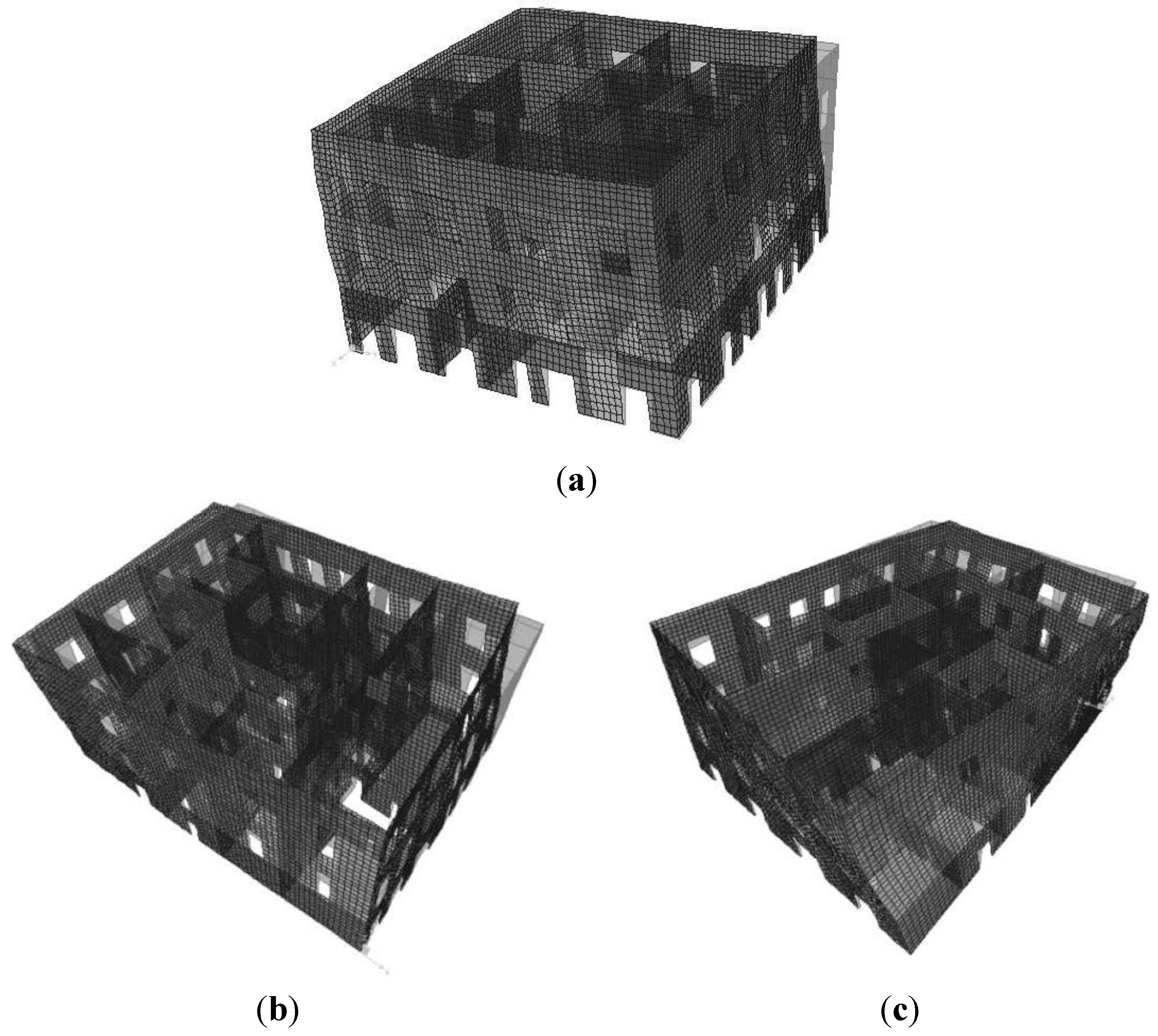
The first eigenfrequency of the building is related to a vibration mode with a participating mass ratio of 70% and is completely translational in Y direction as it can be evidenced by the deformed shape depicted in Figure 6a. The deformed shapes of the building corresponding to the second and third modes (see Figure 6b,c) show a torsional shape of the building, with a prevalent translational component in X direction as evidenced by the participating mass ratios of 38% and 31%, respectively.

Figure 6. Main vibration modes of the structure in the fixed-base FE model: (a) First mode; (b) Second mode; (c) Third mode.

Figure 6. Main vibration modes of the structure in the fixed-base FE model: (a) First mode; (b) Second mode; (c) Third mode.

As highlighted by the experimental results too, the numerical frequency in Y direction (4.7 Hz) is slightly lower (about −10%) than the second and third frequencies characteristic of the X direction (5.13 and 5.79 Hz), that confirms the tendency of the building to be more deformable in the direction Y parallel to the shorter side (see plan in Figure 2a).

The higher numerical modes are characterized by very low participating mass ratios and the deformed shapes of the building show that they are local modes, since they regard single walls.

When the underground level is added to the fixed-base model, the deformability of the structure clearly increases, with an increment of about 16% and 12% in the first vibration period along the Y and X direction, respectively, as reported in Table 3 for the second model.

The first three vibration modes are similar to the ones of the fixed-base model (model 1), even if some differences in the mass participating can be observed (i.e., the mass participating in X direction increases in the second mode and decreases in the third). Moreover, a fourth and a fifth mode in Y and X direction, respectively, are better identified in this model, but they are characterised by a low amount of mass participating (15% and 12%) and, thus, they can be considered as local modes.

Table 3. Period, frequencies and modal participating mass ratios for the FE model of the building with the underground floor.

Mode	Period	Frequency	Translation (−)			Rotation (−)
	T (s)	f (Hz)	X	Y	Z	RX	RY	RZ
1	0.249	4.02	0.00	0.66	0.00	0.25	0.00	0.26
2	0.220	4.55	0.44	0.00	0.00	0.00	0.11	0.37
3	0.196	5.10	0.21	0.00	0.00	0.00	0.06	0.02
4	0.094	10.65	0.00	0.15	0.00	0.04	0.00	0.06
5	0.088	11.40	0.12	0.00	0.03	0.03	0.01	0.06
6	0.083	12.02	0.00	0.00	0.07	0.07	0.03	0.00
7	0.083	12.08	0.01	0.00	0.54	0.26	0.34	0.01
Sum participating mass			0.78	0.81	0.64	-	-	-

Table 3. Period, frequencies and modal participating mass ratios for the FE model of the building with the underground floor.

Mode	Period	Frequency	Translation (−)			Rotation (−)
	T (s)	f (Hz)	X	Y	Z	RX	RY	RZ
1	0.249	4.02	0.00	0.66	0.00	0.25	0.00	0.26
2	0.220	4.55	0.44	0.00	0.00	0.00	0.11	0.37
3	0.196	5.10	0.21	0.00	0.00	0.00	0.06	0.02
4	0.094	10.65	0.00	0.15	0.00	0.04	0.00	0.06
5	0.088	11.40	0.12	0.00	0.03	0.03	0.01	0.06
6	0.083	12.02	0.00	0.00	0.07	0.07	0.03	0.00
7	0.083	12.08	0.01	0.00	0.54	0.26	0.34	0.01
Sum participating mass			0.78	0.81	0.64	-	-	-

For the third model, characterized by the concentrated springs placed under the ground level, periods, frequencies, and modal participating mass ratios associated to the first seven vibration modes, are reported in Table 4. The overall effect of the soil–foundation interaction can be assumed as comprehensive of the part of the building that interacts with the soil both laterally and under the structure.

Table 4. Period, frequencies and modal participating mass ratios for the FE model with concentrated springs.

Mode	Period	Frequency	Translation (−)			Rotation (−)
	T (s)	f (Hz)	X	Y	Z	RX	RY	RZ
1	0.224	4.45	0.00	0.72	0.00	0.32	0.00	0.27
2	0.203	4.92	0.50	0.00	0.00	0.00	0.15	0.41
3	0.179	5.57	0.21	0.00	0.00	0.00	0.07	0.03
4	0.090	11.07	0.00	0.00	0.86	0.46	0.44	0.00
5	0.085	11.72	0.00	0.08	0.00	0.01	0.00	0.04
6	0.082	12.18	0.00	0.04	0.00	0.03	0.00	0.01
7	0.081	12.39	0.08	0.00	0.02	0.00	0.17	0.04
Sum participating mass			0.79	0.84	0.88	-	-	-

Table 4. Period, frequencies and modal participating mass ratios for the FE model with concentrated springs.

Mode	Period	Frequency	Translation (−)			Rotation (−)
	T (s)	f (Hz)	X	Y	Z	RX	RY	RZ
1	0.224	4.45	0.00	0.72	0.00	0.32	0.00	0.27
2	0.203	4.92	0.50	0.00	0.00	0.00	0.15	0.41
3	0.179	5.57	0.21	0.00	0.00	0.00	0.07	0.03
4	0.090	11.07	0.00	0.00	0.86	0.46	0.44	0.00
5	0.085	11.72	0.00	0.08	0.00	0.01	0.00	0.04
6	0.082	12.18	0.00	0.04	0.00	0.03	0.00	0.01
7	0.081	12.39	0.08	0.00	0.02	0.00	0.17	0.04
Sum participating mass			0.79	0.84	0.88	-	-	-

The first vibration mode shows again a well-defined translational modal shape in Y direction (Figure 7a) with a participating mass ratio (72%) lightly higher than the value achieved in the fixed-base scheme (70%, fixed-base Model 1). As in the previous models, the second and third modes evidence a slightly torsional shape of the building, with a prevalent translational component in X direction (Figure 7b,c), even if for the second mode the participating mass ratio in X direction further increases (50% vs. 38% of the fixed-base Model 1), while in the third mode it reduces (21% vs. 30%).

The presence of springs leads to a reduction of the frequencies, i.e., an increase of the period of about 5% and 4% for the first and the second vibration mode, respectively, compared to the values predicted by fixed-base Model 1.

Figure 7. Main vibration modes of the structure in the FE model with concentrated springs at the base: (a) First mode; (b) Second mode; (c) Third mode.

Figure 7. Main vibration modes of the structure in the FE model with concentrated springs at the base: (a) First mode; (b) Second mode; (c) Third mode.

A singularity of the dynamic behaviour of the building modelled with springs is that the fourth mode is characterized by a vertical deformation along the Z direction with a high ratio of participating mass (86%); this mode is clearly caused by the presence of the springs that introduce the possibility of a translation in the Z direction.

The fifth and the sixth mode show again a very low participating mass along the Y direction and, thus, they can be considered as local.

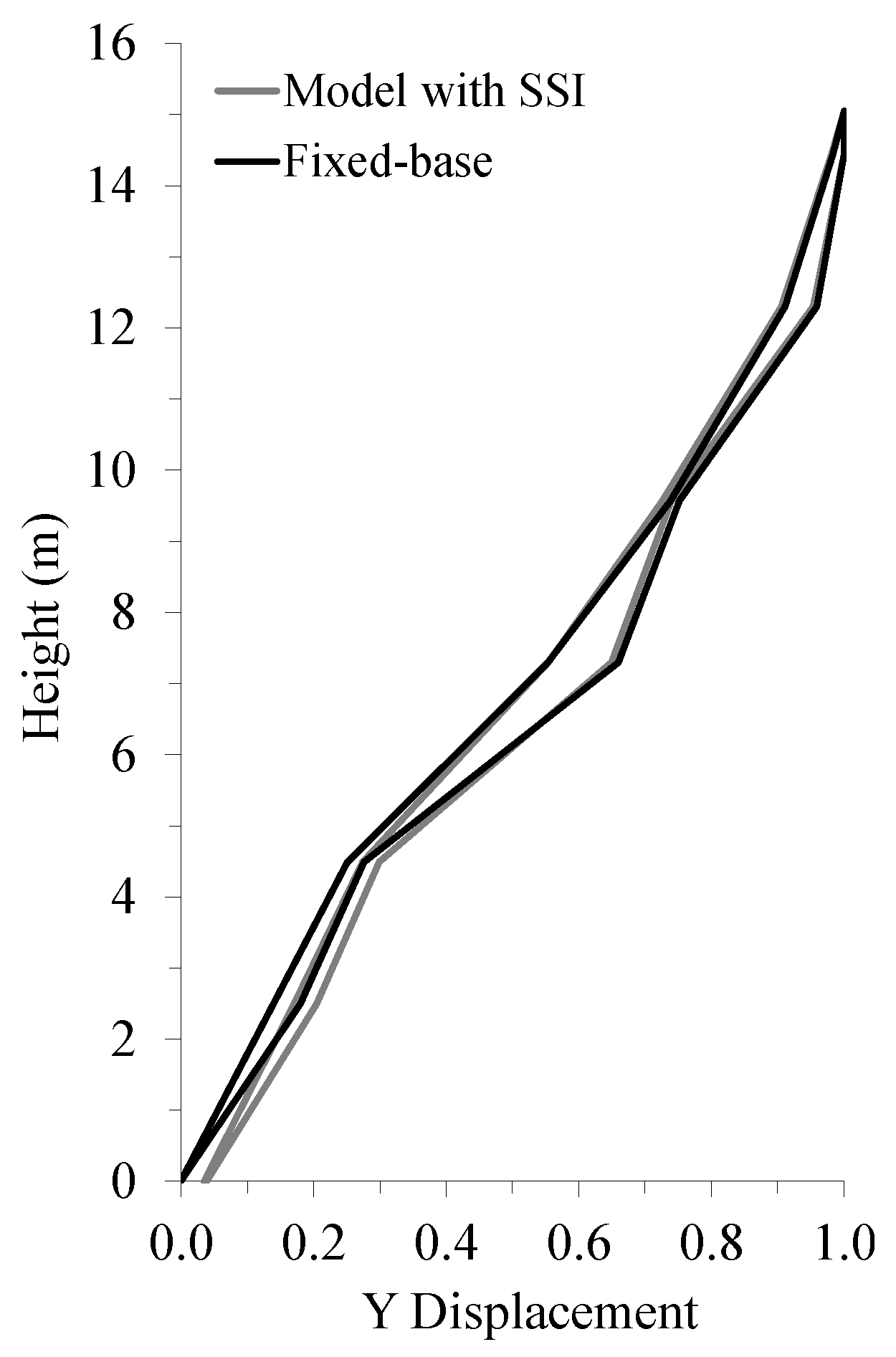
In Figure 8, the first vibration modes in Y direction given by the fixed-base model and the model with springs are compared considering the displacement along the Y direction of the vertical lines at the corners. Since the building has a rectangular plan and is not very tall, the modal shapes cannot be represented by only one vertical and, thus, the deformations along the four corners of the building were plotted. In particular, in Figure 8, the two lines for each model (black lines for the fixed-base and grey lines for the model with SSI) represent the envelope lines (minimum and maximum displacements) of the numerical modal shapes evaluated at each corner of the building. In the model with the springs, the displacements are not zero at the basement due to the presence of the springs; this initial offset dampens along the height and, however, the modal shapes furnished by the two models are quite similar.

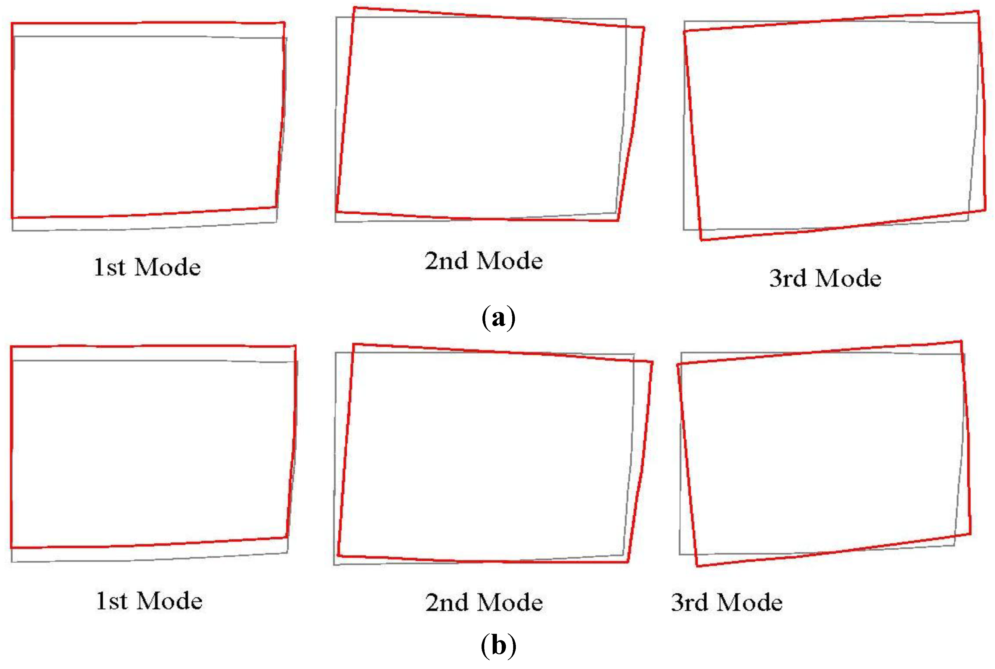
To have more exhaustive comparisons, the first three vibration modes of the fixed-base model and the model with springs have been compared with respect of the positions identified in the plan of the building by the four corners of the structure. In particular, the original and the deformed position of the top of the structure is represented in the pictures reported in Figure 9. Figure 9 shows again that the modes associated to the first two frequencies are translational in direction Y for both models and that the second and the third modes are not only translational in direction X.

Figure 8. Comparison between the first modal shapes (Y direction) at the corners of the building given by the fixed-base model and the model with concentrated springs at the base.

Figure 8. Comparison between the first modal shapes (Y direction) at the corners of the building given by the fixed-base model and the model with concentrated springs at the base.

Figure 9. Comparison between the first three numerical vibration modes of the structure given by: (a) The fixed-base model; (b) The model with concentrated springs at the base.

Figure 9. Comparison between the first three numerical vibration modes of the structure given by: (a) The fixed-base model; (b) The model with concentrated springs at the base.

4.4. Comparison of Linear Dynamic Analysis with Experimental Results

The comparison of the first experimental frequency (4.3 Hz in Y direction) with the first numerical one given by the fixed-base model (4.70 Hz) shows a difference of about 10%. This difference reduces to only 3% in the model with the springs (4.45 Hz) pointing out that there could be an effect of the SSI in making the building more deformable and, thus, more similar to the experimental behavior. Clearly, this is true, if the elastic properties and unit weight of the materials and geometry and loads acting on the structure have been correctly assessed.

About the X direction, all the FE models have provided two frequencies (the second and the third) very close to each other (i.e., 5.13 and 5.79 Hz for the fixed base model and 4.92 and 5.57 Hz in the FE model with springs) and characterized by different participating mass (38% and 31% for the Model 1 and 50% and 21% for Model 3 with springs). The second experimental frequency in X direction (4.7 Hz) is comparable with the values of the second numerical frequency in X direction and, as occurred for the Y direction, is again closer to the value predicted by the model with springs (4.92 Hz). On the contrary, the third numerical frequency in X direction does not correspond to any experimental values and could be related to type of finite element used in the modelling strategy. Similar linear dynamic analysis carried out by a different FE model made of brick elements instead of shell [24] furnished, indeed, slightly different results, since only one frequency was individuated in X direction corresponding to a pure translational vibration mode very similar to the one detected in Y direction and with the same participating mass. This result, joined to the regularity of the building and to the results of the in situ dynamic tests that allowed identifying only two clear uncoupled translational modes in direction Y and X (phase equal to 0), would confirm that the third numerical frequency is not realistic, but has to be attributed to the second mode. Moreover, a confirmation of this hypothesis is the fact that the sum of the participating mass for second and third modes in X direction is comparable with the mass participating associated to the first frequency in Y direction (71% vs. 72% for the model with springs).

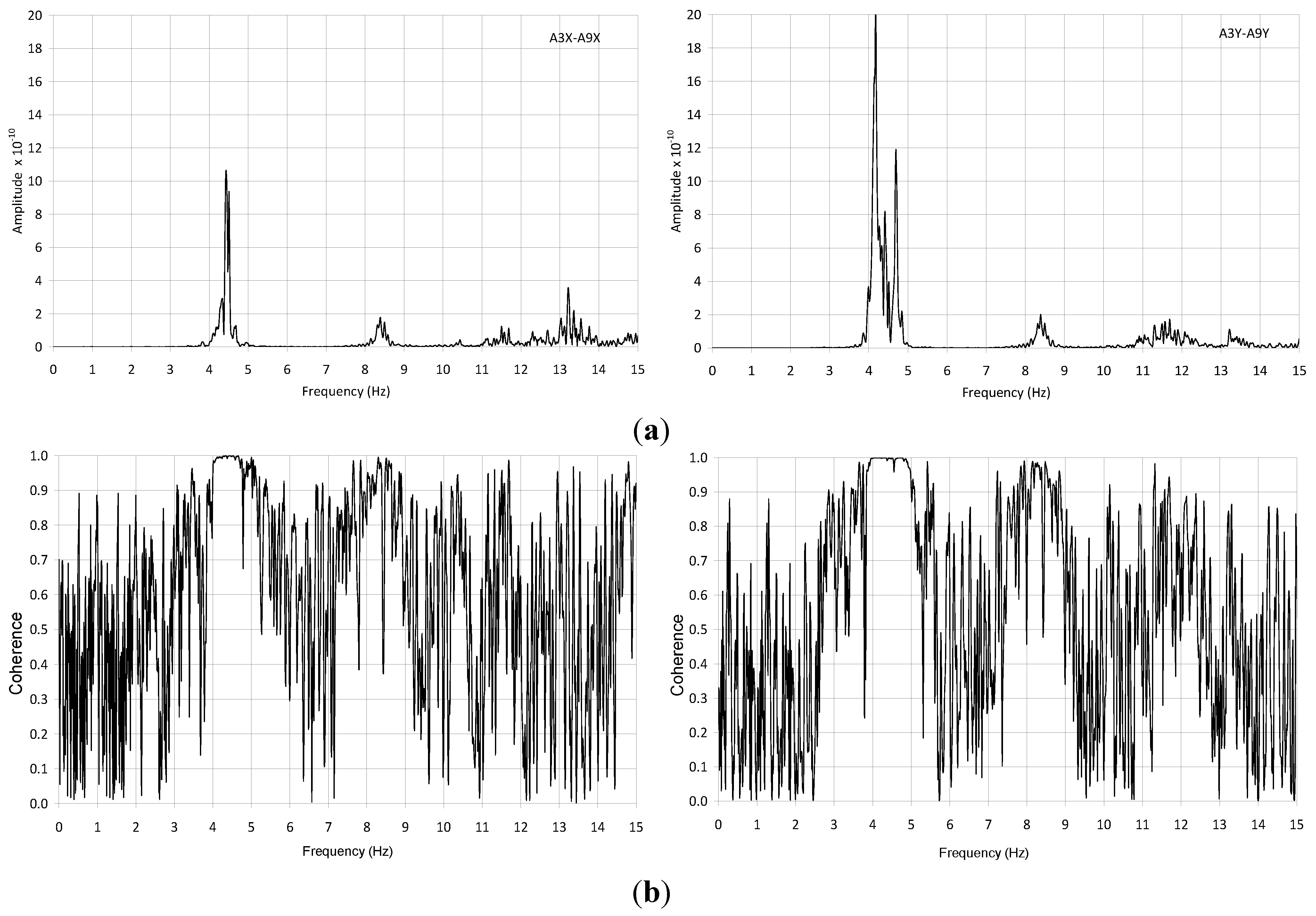
In Section 3.3, it was observed that only the first two frequencies can be reliably identified by means of the experimental measures, since both in X and Y direction higher order frequencies individuated in the ranges 8.0–8.5 Hz were characterized by low amplitude of cross spectra and lower performing values of coherence and phase. This uncertainty about the effective existence of vibration modes of the building associated to higher order frequencies is also confirmed by the absence of a clear correspondence of such frequencies in the numerical results. However, if a third experimental mode really exists at a frequency ranging in 8.0–8.5 Hz, it could be significant of some local phenomena occurring in the real behaviour of the building which are not reproduced in the FE model. Such local phenomena, as for example the lack or the ineffectiveness of connections between walls and floors, could be detected, and thus reproduced in the model, if a detailed relief of the damage state of the building has been done, but for the current level of knowledge of the building none of these phenomena has been evidenced.

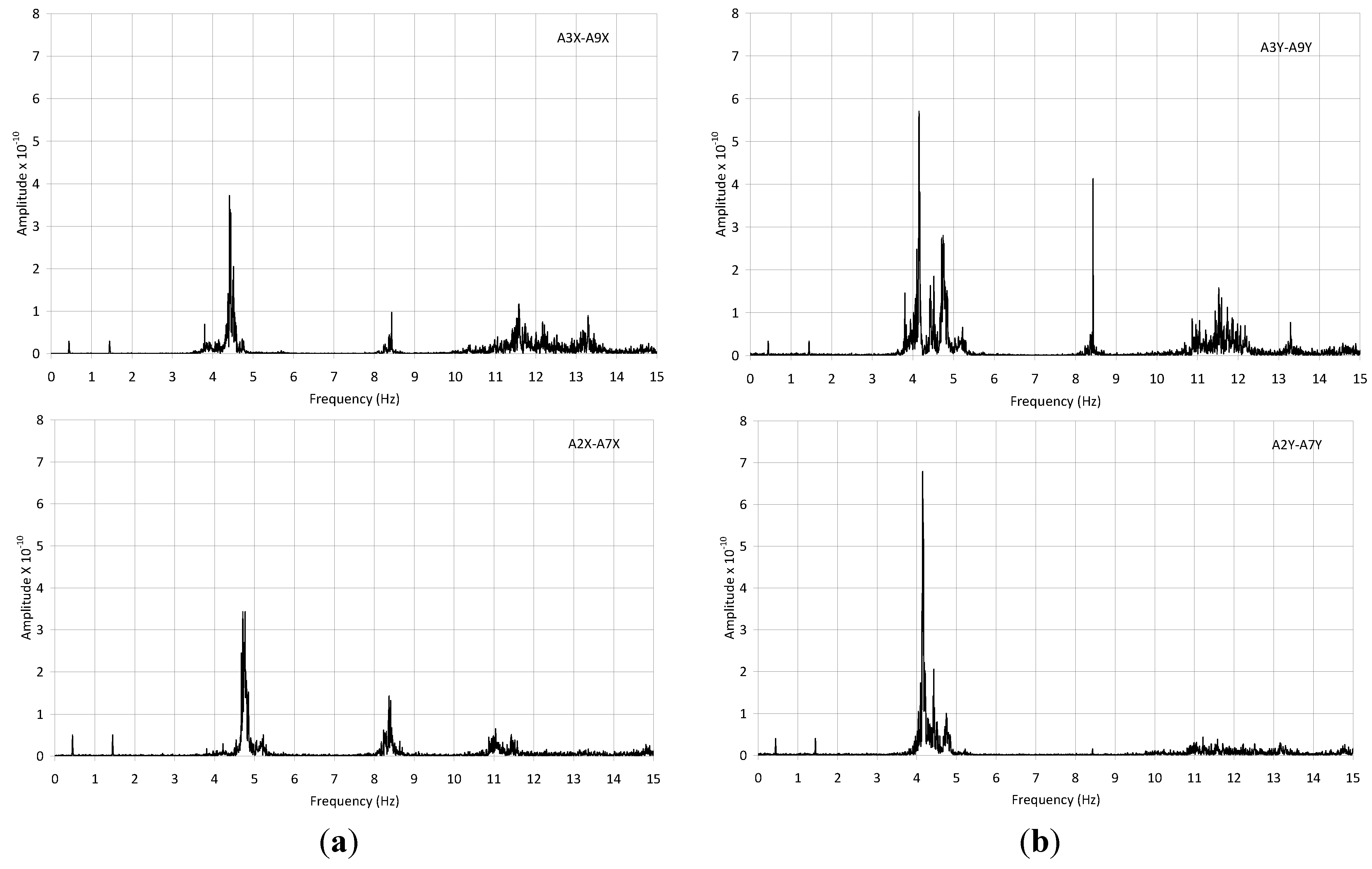
The experimental frequencies detected in X and Y directions in the ranges 11–14 Hz, especially in the measures acquired under environmental conditions, could be associated in the model with springs to the fifth mode associated to the frequency of 11.7 Hz and a mass participating in Y direction of about 8% and to the seventh mode associated to the frequency of 12.4 with a mass participating in X direction of about 8%. However, for such modes the reduced amplitude of the cross-spectra experimentally observed and the low amount of mass participating given by the models lead to considering both of them as negligible.

In conclusion, the comparison between the frequencies assessed experimentally with the numerical values predicted by the FE models has evidenced that only the first two modes can be reliably identified. Moreover, considering the experimental uncertainty and the influence of the FE model adopted, a good agreement between experimental and numerical results has been achieved for the chosen values of elastic properties of the materials and of mass acting on the structure and taking into account the SSI.

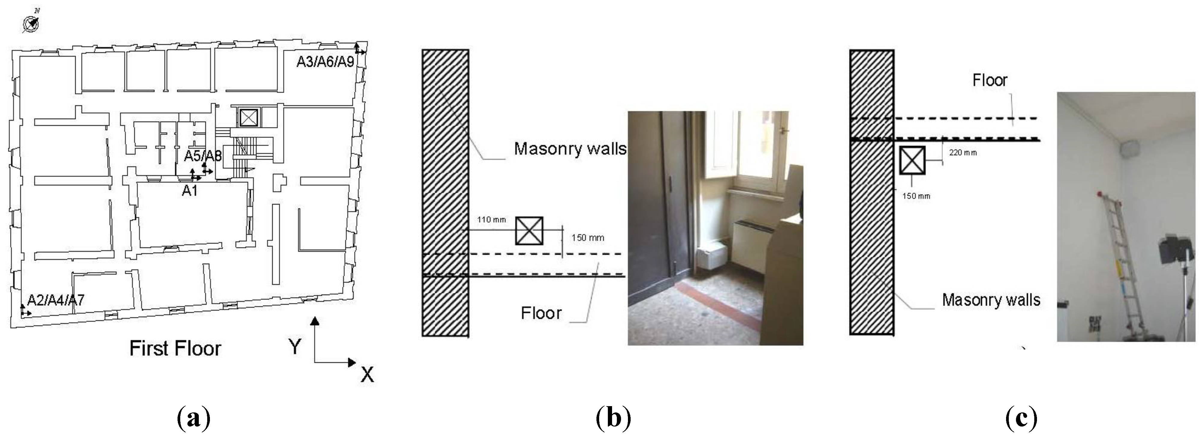
In Figure 10 and Figure 11, the first and the second experimental vibration modes of the structure are depicted, respectively, and compared with the numerical ones given by the fixed-base model and the model with springs. In particular, the normalized displacement of the three instrumented vertical lines have been considered, namely corresponding to the central position (sensors A1–A5–A8), the northern (sensors A3–A6–A9) and the southern (sensors A2–A4–A7) corners of the building. The experimental displacement measured in correspondence of the first and second experimental frequencies (4.3 Hz in Y direction and 4.7 Hz in X direction) have been normalized to the measure of the sensor placed at the top (A8, A9, and A7 for the three vertical lines, respectively). The experimental displacements of first vibration mode measured by the sensors of each vertical in Y direction have been directly compared in Figure 10 with the theoretical ones given by the two FE models, since the first mode is completely translational in Y direction. On the contrary, in Figure 11, for the second mode, the experimental displacements measured in X direction have been compared with the component in X direction of the displacements given by the two FE models, since the numerical second mode was not completely translational in X direction, as previously discussed.

Figure 10. Experimental vs. numerical first vibration modes in Y direction for: (a) The central line (A1–A5–A8); (b) The northern corner (A3–A6–A9); and (c) The southern corner (A2–A4–A7).

Figure 10. Experimental vs. numerical first vibration modes in Y direction for: (a) The central line (A1–A5–A8); (b) The northern corner (A3–A6–A9); and (c) The southern corner (A2–A4–A7).

Figure 11. Experimental vs. numerical second vibration modes in X direction for: (a) The central line (A1–A5–A8); (b) The northern corner (A3–A6–A9); and (c) The southern corner (A2–A4–A7).

Figure 11. Experimental vs. numerical second vibration modes in X direction for: (a) The central line (A1–A5–A8); (b) The northern corner (A3–A6–A9); and (c) The southern corner (A2–A4–A7).

The numerical vibration modes are somewhat more consistent than the experimental ones for both frequencies, especially for the displacement measured at the first floor. The larger deformability introduced by the springs placed at the ground floor only leads to a displacement shift at the basement in the model with SSI, while the shape for height is quite similar.

Notwithstanding the small difference in modal shape and frequencies (only 10%) obtained for the case at hand, the model with SSI is surely a better representation of the structure, since it allows considering the effect of the subsoil which contributes to the real dynamic behaviour of any building. The examined case study is, indeed, representative of a complete approach which accounts also for SSI in the modelling.

Other types of structure, such as tower or very deformable buildings, can be even more susceptible to SSI and it is important to model this phenomenon in evaluating their dynamic behaviour [32,36].

Finally, it is worth noting that further dynamic analyses carried out with the FE model with springs evidenced that as the stiffness of the springs reduces, the second vibration mode becomes more regular and shows a well-defined translational shape also in X direction, similarly to the first vibration mode in Y direction. In addition, the third torsional mode disappears and is substituted by the translational mode along the Z direction which, for the adopted value of spring stiffness, is the fourth one (see Table 4).

In conclusion, the analysis of the vibration modes confirms the necessity of introducing the SSI to have a more reliable model. Such a model may be later used for further dynamic and non-linear numerical analyses.

5. Conclusions

The structural analysis of historical masonry buildings is a complex matter, since each construction is a stand-alone system, designed and erected for being a singular case. Dynamic in situ tests combined with continuous monitoring of the building is an innovative, effective and non-invasive procedure able to assess the overall dynamic behaviour of the structure in terms of main vibration modes and eigenfrequencies.

For the case study herein presented, starting from the interpretation of experimental data coming from a permanent dynamic monitoring system installed on the building by the Italian Department of Civil Protection as alert for medium-high seismic events, the frequencies associated with the first two vibration modes of the building have been identified with sufficient accuracy by means of basilar instruments of OMA. Also, the experimental vibration modes of the building associated with the first two frequencies and computed along three instrumented corners have been obtained.

Both experimental frequencies and vibration modes have been compared to the results of linear modal analyses carried out through three refined three-dimensional FE models of the building made of shell elements. The models were aimed to investigate also the role of the subsoil in modifying the dynamic response of the building. In particular, the effect of the subsoil has been introduced by means of concentrated translational and rotational springs placed at the ground floor of the building. The values of stiffness of such springs have been assessed considering well-known literature formulations and based on the mechanical properties of the subsoil.

The comparisons between experimental and numerical results allowed evidencing some flaws both regarding the experimental measures and the FE model. In view of the experimental uncertainty about the identification of higher order modes characterized by a low amount of participating mass and the influence of the type of FE element adopted in the numerical predictions, indeed, only the first two modes of the examined building have been reliably identified.

A good agreement between experimental and numerical results has been finally achieved for the chosen values of elastic properties of the materials and of mass acting on the structure, also taking into account the SSI by means of concentrated springs at the basement.

Even if for the examined building the variation of frequencies and modal shape observed when the SSI is taken into account is not high, a FE model with SSI is surely a better representation of the structure. The examined case study can be considered as representative of a complete approach which accounts also for SSI in the modelling since it allows considering the effect of the subsoil which contributes to the real dynamic behaviour of any building. On the other hand, other types of structure (tower or very deformable buildings) can be even more susceptible to SSI and it is important to model this phenomenon in evaluating their dynamic behaviour.

It is worth pointing out that many parameters may influence the results of modal analyses in terms of both frequencies and modal shapes. In particular, the type of selected finite elements (i.e., a model made of three-dimensional elements is expected to provide higher frequencies compared to a model made of shell elements, since the simulated building is overall more stable), the uncertainty about the geometry of the building, masonry elastic properties (i.e., for the case at hand the values of Young’s modulus of masonry should be better assessed with specific in situ inquires) and unit weight, the permanent and the accidental loads acting on the building, the mechanical properties of subsoil. Each one of the above factors is worth being singularly examined. This aspect is beyond the scope of this paper, primarily devoted to highlighting the role of the foundation soil in the dynamic identification process of a masonry structure.

The obtained results represent the starting point for future analyses aimed at assessing the seismic safety of the building, located in one of the most seismically active zones of Italy (Sannio).