Article

Impact of Public Space in Primary and Secondary Schools Based on Natural Visibility Ratio

by
Feng Liu
1,*,
Hao Zhou
1,
Jiangtao Xie
1,
Yue Tang
2 and
Shuyu Liu
1
1
School of Architecture, Nanjing Tech University, Nanjing 211816, China
2
Department of Architecture and Built Environment, Faculty of Engineering, University of Nottingham, Nottingham NG7 2RD, UK
*
Author to whom correspondence should be addressed.
Buildings 2025, 15(9), 1472; https://doi.org/10.3390/buildings15091472
Submission received: 20 February 2025 / Revised: 20 April 2025 / Accepted: 24 April 2025 / Published: 26 April 2025
(This article belongs to the Section Architectural Design, Urban Science, and Real Estate)

Abstract

Campus safety is an essential prerequisite for the development of the education system, as it directly impacts the security of life and property for a significant number of students and faculty members. In recent years, the safety of primary and secondary schools has garnered considerable attention from policymakers and architects, necessitating rational design methods to develop effective strategies that optimize the campus environment. This study utilizes algorithmic simulations, spatial analysis, and statistical methods to examine the relationships between the layouts of buildings, public space morphology, and campus safety. This study analysed 53 schools, which are mainly located in urban areas of China, and variations in their design that were generated through computational modelling. It revealed that, while the architectural layout has a relatively limited direct impact on the safety of school public spaces, the shape and scale of these spaces can significantly enhance their safety performance by allowing for improved natural surveillance. The findings of this study underscore the critical importance of controlling the form and configuration of buildings and public spaces in school design, providing a robust foundation for safety-oriented campus planning.

1. Introduction

1.1. The Paradox of Security and Pedagogy in Campus Design

The safety of primary and secondary school campuses has emerged as an increasingly pressing global concern, especially in the wake of incidents involving violent attacks and bullying [1,2,3]. As school safety concerns escalate worldwide, designing educational environments now represents a critical challenge that requires a careful balance between meeting security imperatives and meeting developmental needs. In response, China has implemented comprehensive management strategies that have yielded significant progress in incident reduction. The Ministry of Education of the People’s Republic of China, in collaboration with other relevant departments, has launched a series of initiatives to address school safety concerns [4]. Central to this approach is the principle of target hardening—strengthening the physical security features of spaces to deter threats—which has driven substantial investments in security infrastructure upgrades [1,5]. These upgrades include the widespread installation of surveillance networks, biometric access controls, and perimeter fortification systems.
Contemporary approaches increasingly reveal a fundamental tension between physical protection measures and the creation of nurturing learning ecosystems. While infrastructure hardening strategies such as the use of surveillance technologies and access control systems have demonstrated operational effectiveness, emerging scholarship questions their long-term impacts on adolescent development and spatial functionality. Excessive reliance on such measures in specific cultural contexts risks undermining efforts to foster inclusive school climates, and adverse effects on students’ daily experiences have been documented [2,6,7]. The broader efficacy of this approach remains contested, particularly in transitional zones between controlled classrooms and dynamic communal areas. Here, rigid security frameworks often impede the spontaneous social interactions that are fundamental to youth development, revealing a misalignment between risk mitigation and educational imperatives [6].
The design of a campus should be closely integrated with the development of comprehensive school security systems. The crime prevention through environmental design (CPTED) principles have emerged as a theoretically promising framework for reconciling these competing demands. The CPTED principles incorporate three interrelated strategies: access control, natural surveillance, and territorial reinforcement. These principles have been widely applied in various contexts, including educational settings [8] and commercial environments [9], and have demonstrated effectiveness in numerous studies [5,10,11]. Additionally, several studies have examined the application of the CPTED principles to the assessment of school safety, highlighting the critical role of natural surveillance [12]. The U.S. Centres for Disease Control and Prevention (CDC) have adopted CPTED as a framework for preventing school violence, developing the CPTED School Assessment (CSA) tool, which integrates five key principles: natural surveillance, access management, territoriality, physical maintenance, and order maintenance. This tool has been utilized to investigate school violence and safety concerns among middle school students, proving its efficacy in guiding environmental modifications to reduce violence and enhance the overall safety in schools [13].
Early adopters like Scheider and Kitchen demonstrated CPTED’s potential in schools through observational studies linking spatial transparency to reduced bullying incidents [14]. Contemporary research falls into two main categories: one body of the existing literature offers design recommendations and strategies based on extensive comparative analyses [15,16,17], while another strand focuses on the quantitative assessment of spatial safety, facilitating efficient and precise case comparisons [12,18,19,20]. Central to CPTED is the principle of natural surveillance, which aims to deter criminal activity by maximizing the visibility within a space. Improved environmental visibility not only reduces the likelihood of criminal behaviour but also enhances the capacity of authorities for rapid detection and intervention when incidents occur.
However, the limitations of traditional CPTED applications have been well-documented. Cozens’ cross-cultural studies exposed fundamental implementation challenges in educational contexts, particularly the tension between territorial definition and spatial inclusivity [21]. He further notes the inherent difficulty in proving the strategy’s effectiveness, which has hindered large-scale governmental investment and intervention. Similarly, Ekblom critiques the current state of CPTED, highlighting its limitations such as imprecise definitions, disciplinary isolation, rigidity in its application, a lack of evidence-based practices, and the neglect of social and contextual factors [22]. His research highlights the importance of understanding the complex relationships between the physical environment and human behaviour. He also emphasizes the role of social factors and advocates for evolving CPTED methodologies to better address modern security challenges [23].
The architectural implementation of the CPTED principles reveals three critical gaps in current school design practices:
  • Oversimplified safety zoning: Traditional binary classifications of “safe/unsafe” zones fail to account for the gradient nature of the spatial permeability that is required for adolescent socialization. This rigid framework ignores transitional zones that facilitate both security and social interaction;
  • Excessive visibility and its paradoxes: While visibility is a cornerstone of CPTED, overreliance on surveillance technologies (e.g., cameras) and transparent designs can disrupt peer socialization and raise privacy concerns [2,24]. Transparency, intended to enable casual supervision, may inadvertently expose students to unwanted attention or interruptions, undermining their perceived safety [6]. Visual connectivity between spaces can also yield counterproductive effects, such as bystander fixation during conflicts [25];
  • Isolated security interventions: Conventional approaches prioritize fragmented measures over holistic spatial performance. These interventions often distort spatial layouts, creating compensatory blind spots and compromising their educational functionality.
This tension between safety optimization and spatial integrity demands a paradigm shift in safety-focused design. Research indicates that the majority of campus safety incidents—such as bullying, harassment, and violence—occur not in classroom spaces, but in public spaces like courtyards and recreational areas [25,26]. These dynamic environments, characterized by high student interaction and congregation [27,28,29], require distinct design priorities.
Emerging research highlights the underappreciated role of geometric properties in mediating security outcomes [30]. However, the mechanisms by which morphological elements influence the natural surveillance efficacy—and thereby overall safety—of a space remain poorly characterized. A critical challenge lies in optimizing the spatial visual connectivity of a space to enhance its security without compromising its functional utility or social interaction capacities, a balance that requires the careful calibration of visibility thresholds and programmatic adjacencies.
Therefore, this research addresses these challenges by focusing on public spaces within primary and secondary schools, exploring spatial optimization approaches to enhance safety. By examining the relationship between spatial features and safety outcomes, this study aims to provide valuable insights into how architectural interventions can help prevent safety incidents and improve the overall security of campuses.

1.2. Computational Morphology: Bridging Design and Security

The safety-oriented design discussed in this study requires the integration of two research trajectories: one is the morphological approach, which analyses the impact of spatial physical characteristics, and the other is the application of computational methods in architecture, enabling more precise spatial research. Morphology encompasses the physical characteristics and structural composition of the built environment, constituting a fundamental aspect of urban planning and design [31,32,33]. Initially introduced in urban studies, the concept of urban morphology is centred on analysing cities as assemblies of abstract elements and examining their form, structure, and evolution [31,34]. The term “morpho” was proposed to address design-related issues, including the type of area under assessment and the purpose of such evaluations [34]. Morphological typology analysis provides evidence-based guidance for navigating the inherent trade-offs between geometric regularity and spatial functionality. Computational methods leverage digital tools (e.g., generative algorithms, computer graphics) to enable granular spatial investigations [35,36]. These techniques facilitate the predictive modelling of visibility metrics, risk simulations, and data-driven optimizations [37,38].
At the core of this synthesis lies three methodological advancements:
  • Space syntax: Introduced by Hillier and Hanson, space syntax is a theoretical and computational approach that applies graph theory to analyze spatial configurations [39,40]. Unlike traditional architectural analyses which are focused on the physical form of buildings, space syntax emphasizes topological relationships—how spaces connect, integrate, and sequence within a system [41]—and builds bridge a between spatial features and behavioral patterns [42]. Key elements in space syntax include axial lines, convex spaces, integration, connectivity, and depth. These metrics reveal how spatial arrangements influence the flow of activities, social behaviours, and interaction patterns [43];
  • Parametric modelling: parametric modelling translates spatial relationships into mathematical formulations, shifting design from being qualitatively subjective to being quantitatively rigorous. Parametric design facilitates exploring design alternatives and optimizing spatial configurations based on a set of predefined constraints [44]. It is particularly useful for understanding the relationship between geometry and spatial performance, and includes visibility, circulation, and environmental factors;
  • Computational methods and algorithms: These methods involve the use of computer algorithms to solve complex design problems. One popular tool is evolutionary algorithms (EAs), which can automate the exploration of complex design spaces, optimizing solutions for multi-objective problems [35]. Rule-based generative systems encode design logic into computational workflows, enabling data-driven spatial analyses and iterative refinements.
The integration of computational methodologies has reoriented the implementation of CPTED [45]. By reconceptualizing building footprints and public space configurations as dynamically modifiable elements, designers can systematically evaluate how geometric interventions propagate through spatial systems. This reveals previously overlooked relationships between architectural forms and security outcomes, such as how the morphologies of campus public spaces influence both the natural surveillance potential and social interaction patterns.
Contemporary scholars have significantly expanded these computational frontiers. Nubani and Wineman employed space syntax measures to investigate the geographical patterns of four criminal behaviour types and identify street segment characteristics that influence crime incidence [46]. Mostafa conducted a case study in Bojnourd, examining how physical elements in educational spaces impact students’ sense of security [47]. His study identified supervision as one of the most critical factors that influences campus safety. Mina et al. integrated space syntax with CPTED to examine how these frameworks, alongside demographic variables, influence residents’ outdoor physical activity levels and perceptions of safety [45]. Their study highlights the strengths of space syntax in safety-related research: it clearly and precisely demonstrates the relationship between spatial attributes (e.g., connectivity, accessibility) and the perceived safety of a space, providing a quantitative foundation for linking urban design features to human behavioural outcomes.
The fusion of computational and morphological methodologies creates new possibilities for evidence-based campus design. Through the iterative simulation of architectural variants, designers can identify configurations that optimally balance competing demands of security, functionality, and social development.
Building upon this interdisciplinary framework, this article explores the intersection of school design and campus safety. A set of 53 case studies was selected to investigate the relationship between the morphology of public spaces and the safety of campuses. To facilitate our quantitative analysis, public spaces were abstracted into geometric figures, providing a clear representation of the physical environment and its impact on safety. This approach is grounded in spatial analysis principles, where geometric simplifications enable the objective evaluation of underlying design principles.
This paper commences by describing the employed method, including the dimensions from which the design of schools is studied and the evaluation approach for public space security. The details of the school cases used and the criteria for selection are presented in Section 2. The analysis of school design is presented from two perspectives: campus layouts and public space morphological features, which are discussed, respectively, in Section 3. Finally, this article concludes with a discussion about the quantitative relationships between spatial features and campus safety, along with actionable design recommendations.

2. Material and Methods

This study extends CPTED (crime prevention through environmental design) theory by investigating how campus safety in primary and secondary schools relates to the spatial features of public spaces. The spatial analysis examines two critical aspects of school design: campus layout configurations and public space morphology [48]. Recognizing that layout modifications inherently influence the morphological characteristics of public spaces. The research first addresses the impact of spatial organization patterns before progressing to detailed morphological analysis. By systematically investigating the application and extension of CPTED theory in architectural design through the generation of multiple spatial variants via algorithmic methods, integrated with space syntax analysis and statistically rigorous two-tailed hypothesis testing evaluation. The methodological workflow is presented in Figure 1.

2.1. Natural Visibility Metrics in Campus Safety Evaluation

According to the crime prevention through environmental design (CPTED) theory, natural surveillance is recognized as a pivotal factor that influences spatial safety [49]. And it is desirable in many contexts as it has the potential to reduce crime rates and generate a sense of safety [50,51]. Building on this principle, the concept of natural visibility has been introduced [19]. Natural visibility refers to the absence of visual obstructions between two points in a space, allowing these points to be mutually visible. The natural visibility level quantifies the quality of visual conditions at a given point within a space. Evaluating the overall natural visibility level of a space involves assessing the extent to which sightlines remain unobstructed throughout the area. Higher levels of natural visibility in a campus environment correlate with enhanced spatial safety. Further, it affects the activity pattern of students.
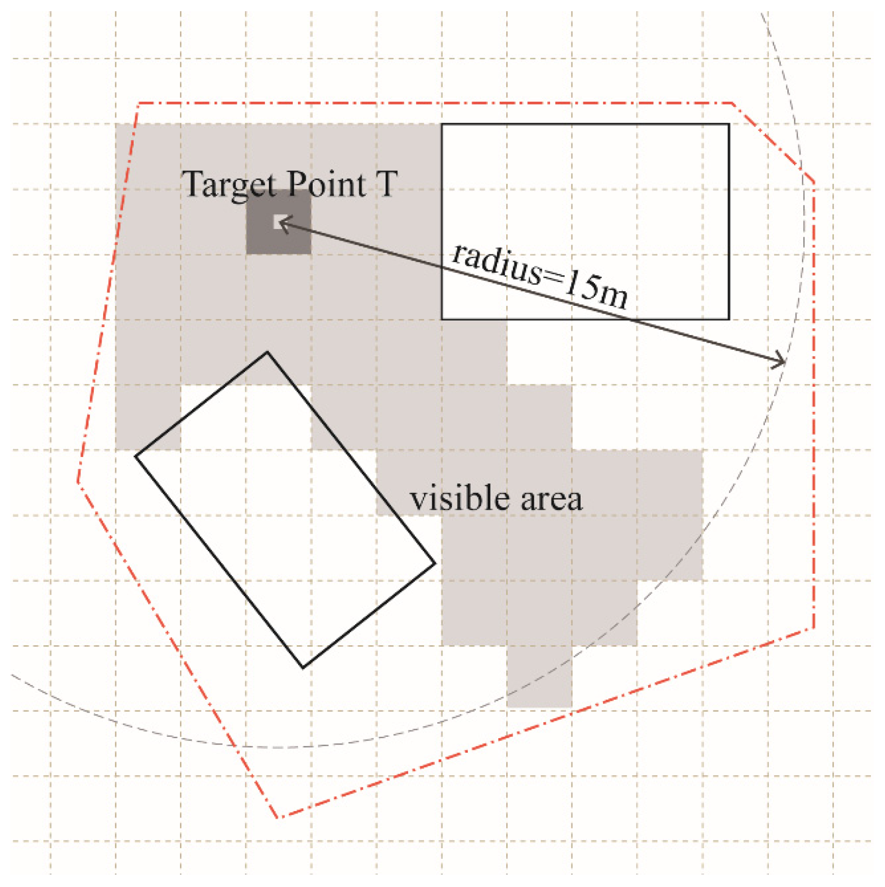
The natural visibility ratio is a quantitative measure of the natural visibility level and the safety of public spaces on a campus. First, the maximum viewing distance for natural observation is determined based on the physiological characteristics of the user population as Figure 2 shown, i.e., the distance from the observation point (OP) to the target point (TP). Within this distance range, multiple OPs may exist for a TP. If there are no obstructions between the TP and the OP, the OP is included as a valid observation point (VP). The ratio of the total number of VPs to the total number of all OPs is the natural visibility ratio Rv, which measures the natural visibility level of that TP. If the Rv of a TP is lower than 0.5, it is considered to have a low level of visibility, indicating inadequate natural surveillance and potentially compromising security [19]. The arithmetic mean of the Rv values for all TPs within the space is then calculated to quantify the overall natural visibility level of the space.
Adolescents constitute the primary users of primary and secondary school campuses. Previous research has demonstrated that the human eye is capable of recognizing individuals and accurately interpreting events within a distance of 15 m [52]. Consequently, 15 m is widely regarded as the effective surveillance distance in safety-related studies [38]. This distance is further corroborated by Anastasia Loukaitou-Sideris’ research on natural surveillance distances [53]. Moreover, the Code for Design of Schools recommends 15 m as the optimal distance for reducing visual interference [48]. Based on these findings, this study adopts 15 m as the maximum natural observation distance in assessing the natural visibility level of outdoor public spaces on campuses. Additionally, taking into account the characteristics of adolescents, visual obstructions on campuses are defined as opaque objects with a height of 1.2 m or greater [19]. The calculation and output of the natural visibility level were automated using Python programming to facilitate batch processing.
Campus safety optimization presents a complex challenge due to the inherent tension between localized risk mitigation and global solution optimization, particularly given the empirical correlation between safety incidents and areas characterized by limited teacher supervision or compromised visibility [26]. This study identifies spatial zones with substantially reduced safety performance as high-occlusion spaces, and these are operationally defined as having natural visibility ratios (Rv) that are consistently below the 0.5 threshold [19]. These critical areas warrant prioritized spatial redesign interventions to address inherent safety vulnerabilities. From a computational perspective, the harmonic mean demonstrates a unique sensitivity to extreme low-value outliers within datasets. This property makes its adoption particularly advantageous for calculating average natural visibility ratios (Rvh), as high-occlusion spaces exert disproportionate influence on the resultant metric. Consequently, Rvh serves as a more robust indicator of occlusion risks compared to conventional arithmetic mean calculations (Rva). The enhanced discriminative capacity of Rvh enables more precise identification of spatial configurations that require safety interventions, thereby improving campus safety planning efficacy. For systematic reference, this research maintains distinct notation: Rva denotes the arithmetic mean of natural visibility ratios, while Rvh represents their harmonic mean.

2.2. Algorithmic Iteration and Spatial Analysis for Campus Layout Optimization

The study employs a hybrid generative-statistical methodology. First, algorithmic iteration generates numerous variants of building layouts and public space forms. For building layouts, variants derive from sampled school layouts. For public spaces, stochastically generated shapes are first analyzed, and the results are then substituted into sampled schools for validation. Finally, multiple linear regression models are used to determine the combined effects of layout and morphology on safety outcomes.

2.2.1. Campus Layout Configuration Generates Simulation

In architecture, the building layout pertains to the spatial organization and configuration of both interior and exterior spaces within a structure [54]. This encompasses the positioning and interrelationships between internal and external areas. The building layout plays a crucial role in the design process as it determines the functionality of the building, its interaction with the surrounding environment, and the user experience. It significantly impacts practical aspects such as usability, efficiency, and safety, as well as the emotional and aesthetic responses elicited from users and the broader environment [55,56]. Broadly speaking, the building layout involves multiple factors, including horizontal and vertical configurations [56,57,58,59]. These introduce complexities that present challenges for further research:
1)
Although the functional configuration may change, the building form generally remains unchanged, and, consequently, the morphology of public spaces typically remains consistent as well;
2)
When changes in the functional configuration lead to alterations in the morphology of public spaces, the building form is often modified concurrently. In such instances, the influence cannot be attributed to a single factor, making it challenging to evaluate;
3)
If vertical changes in the building layout entail modifications to the spatial relationships between different buildings, both the building form and density will undergo corresponding adjustments. In these scenarios, the variables are no longer singular.
This study adopts a restricted definition of building layout, concentrating exclusively on the horizontal configurations of structures.
The quantification of building layout configurations is a persistent challenge in architectural research, primarily due to methodological biases inherent in conventional quantitative approaches. Traditional analytical frameworks are susceptible to systematic distortions arising from selective methodology applications, which potentially compromise the validity of spatial evaluations. To address these limitations, this study proposes an innovative computational approach that employs algorithmic methodology to systematically investigate layout variations. Leveraging Python’s robust computational capabilities, the framework implements were able to control stochastic transformations of architectural configurations through iterative spatial reconfigurations. The developed algorithm extends classical hill-climbing optimization principles [60] through strategic modifications that prioritize comprehensive configuration space exploration over local optimization [61]. By implementing exhaustive state-space sampling rather than directional optimization, this methodology enables rigorous the statistical analysis of emergent spatial patterns while mitigating convergence artifacts. The details of the technical implementation of this computational paradigm and its application in generating architecturally meaningful layout permutations are outlined below.
For the selected campus layout, the current state is denoted as S0. First, one building (or an obstacle) is randomly selected, and is moved in a random direction by a distance ranging from 0.1 to 5 m, resulting in a new state S1. This complete process is denoted as M1. This procedure is expressed as follows.
S 1 = M 1 ( S 0 )
Then, using the same method but with a different displacement vector M2, a new state S2 is obtained based on S1. This procedure continues iteratively until the number of results meets the requirement. Finally, the program ends up with n + 1 samples, ranging from S0 to Sn. For any sample, the following is satisfied:
S i = M i ( S i 1 ) ,   i [ 1 , n ]
This algorithm does not evaluate the reasonableness of intervals between obstacles, and thereby creates both plausible and implausible scenarios. The calculated displacements are relatively conservative since, under specified design conditions, the optimal overall functional layout, including the positioning of teaching, living, and activity areas, is relatively fixed and unlikely to undergo significant alterations. Furthermore, the algorithm does not incorporate building rotation because the orientation of a structure significantly impacts the indoor space utilization. However, for outdoor public spaces, shape changes resulting from either building translation or rotation are considered equivalent in terms of spatial impact.
Using this algorithm, multiple layouts (variants) are generated for each school, collectively forming a group. To facilitate subsequent linear regression analysis, each layout is quantified into a numerical metric through calculation of the z-scores of the Rva and Rvh within its respective group. These metrics are denoted as LYTa (z-score of Rva) and LYTh (z-score of Rvh), serving as standardized indices for comparative analysis. The z-score quantifies how many standard deviations an individual deviates from the mean, normalizing its position within the distribution. In this study, we calculate the z-score of the arithmetic mean of the natural visibility ratio (Rva) for each campus layout variant to assess its relative performance.
Since there is no clear directionality when altering building layouts, each school layout variant may exhibit higher or lower visibility levels compared to the original configuration. The z-score reflects the original layout’s relative ranking within its group. A positive z-score (LYTa > 0) indicates that the original layout outperforms the majority of variants. Conversely, the same applies for the reverse. This standardization mitigates distortions caused by variability in sample ranges (e.g., differences in Rva spans across groups), enabling equitable comparisons of safety performance across diverse campuses. By contextualizing the original layout’s Rva within its group’s distribution, the z-score provides a robust metric for the evaluation design efficacy, independent of other spatial features.

2.2.2. Morphological Features Extraction of Public Space

Converting space into two-dimensional figures is a prevalent method for quantitative analysis in architectural research [56,62]. Campus public spaces can be represented as vectorized geometric figures that delineate the extent of natural visibility. Typically, the inner boundary corresponds to the outer contour of buildings, while the outer boundary aligns with the property or campus perimeter. However, in practical campus settings, lawns that do not obstruct sightlines may be utilized for daily activities but remain underutilized. If located near campus fences, where the boundary of the figure may no longer coincide with the campus boundary (Figure 3), the boundaries of public spaces should be redefined according to specific contextual factors.
By establishing a connection between school public spaces and geometric shapes, this study aims to elucidate the relationship between spatial morphology and campus safety. Morphological evaluation in this research is conducted from two perspectives: density and form. Density primarily concerns the distribution of obstacles within the campus, which generally correlates with the building coverage rate. The forms of buildings in this study have been comprehensively assessed through measurements of geometric shapes.
Compactness is a widely used polygon shape property, and is commonly quantified using the compactness index [63]. It has been widely used to describe the shapes of areas in urban studies [64,65]. A compact polygon has a relatively simple boundary with vertices that are approximately equidistant from the centroid [66]. The compactness index is calculated as shown in Equation (3), which is proposed by Richardson [67].
C I = 2 π A P
It can also be calculated using the Polsby–Popper method [68]:
C I = 4 π A P 2
CI represents the compactness index, A represents the area, and P represents the perimeter (including the external boundary and internal boundaries of the shape). The larger the index, the more compact the area, and the more closely its shape approximates a circle. CI is independent of the size of the shape, but excluding the size may not be suitable for architectural research. For example, when expanding a space in design, it can be either proportionally scaled or combined with another space.
The shape factor is a fundamental parameter in architectural design that quantifies the three-dimensional geometry of a building. It is defined as the ratio of the building’s external surface area, which is exposed to the outdoor environment, to the volume it encloses. A higher shape factor indicates a more complex and irregular building form. For buildings with a flat roof and approximately uniform floor plans across levels, the following equation can be derived:
F S = A r + P 0 × h A b × h = 1 h + P 0 A b A r = A b
FS represents the shape factor, h represents the story height, Ar represents the roof area, Ab represents the building area, and P0 represents the perimeter of each plane. Based on these equations, the form area factor is introduced to describe the 2D shape of a space, and is calculated by the following equation.
F A = μ A × P A ,   μ A = 1   m - 1
FA represents the form area factor, and μA is a constant that transforms FA into a dimensionless number, which can be determined in accordance with different purposes. In contrast to the shape factor, a larger form area factor indicates a more irregular planar shape, or a more fragmentary space.
Python programming was utilized to generate a series of random geometric shapes based on the analysis of real-world school case studies. These shapes can be interpreted as representations of school grounds or sections of public space. The specific algorithm employed is as follows:
(1)
Determine the quantity of edges n, and then generate n degrees ai (i ∈ [1, n]), sorting them in ascending order;
(2)
Generate n distances di. The vertices can be uniquely determined in a polar coordinate system by ai and di. These vertices are then connected sequentially to form a polygon;
(3)
Scale this polygon until its area equals S.
In design practice, plot boundaries are typically defined by surrounding roads. For ease of vehicle movement, roads generally do not have excessive curvature, which thereby limits the complexity of the plot boundaries of most of the studied buildings. Moreover, land shapes with a higher number of edges can often be conceptually simplified. Consequently, n is usually set within the range of 3–9.

2.3. Case Selection

A total of 53 primary and secondary schools were selected for this study, numbered from 01 to 53 (see Appendix A for geographic distribution). The plans of these school are shown in Figure 4. The sample prioritizes spatial diversity, focusing on two key variables—school size and campus layout—to capture a representative spectrum of spatial configurations in public spaces. Schools with flat terrain (average elevation difference less than 1 m within a 15 m observation radius) were prioritized. This criterion ensures unified extraction of spatial features and calculation of natural visibility ratios, minimizing terrain-induced biases while ensuring sufficient representativeness of typical school environments [69].
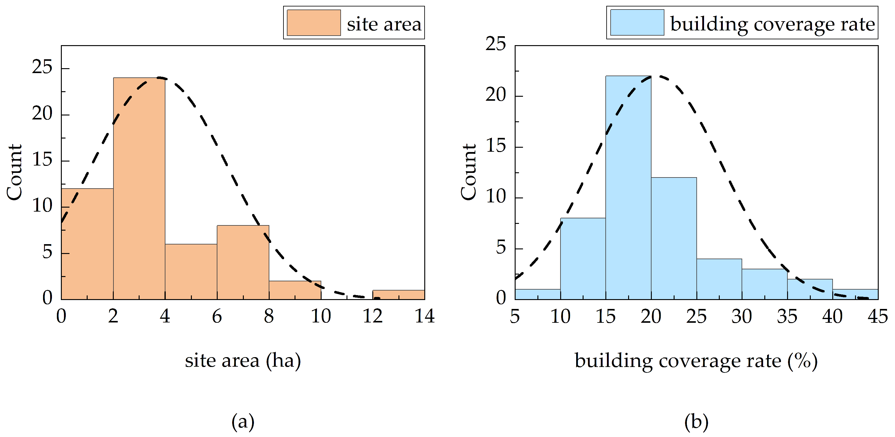
The study sample comprises 53 schools across seven regions, with 40 in Nanjing, 2–4 each in Tianjin, Shenyang, and Harbin, and a single case in Taiyuan. While geographically concentrated in Nanjing, the institutions demonstrate marked heterogeneity in their physical attributes (Figure 5), including their gross floor areas (4000–13,000 m2) and public space typologies.
Morphometric analysis reveals divergent spatial configurations, with site areas and building coverage ratios spanning from compact to expansive layouts (Figure 5). Consistent flat terrain and comparable urban contexts enable the computational abstraction of outdoor spaces as planar environments. This controlled variability in campus size, form, and spatial organization ensures the sample’s representativeness of primary/secondary schools, supporting generalizable conclusions about safety-related spatial determinants.

3. Results

3.1. Building Layout with Natural Surveillance

3.1.1. General Relationships Between Building Layouts and Rva

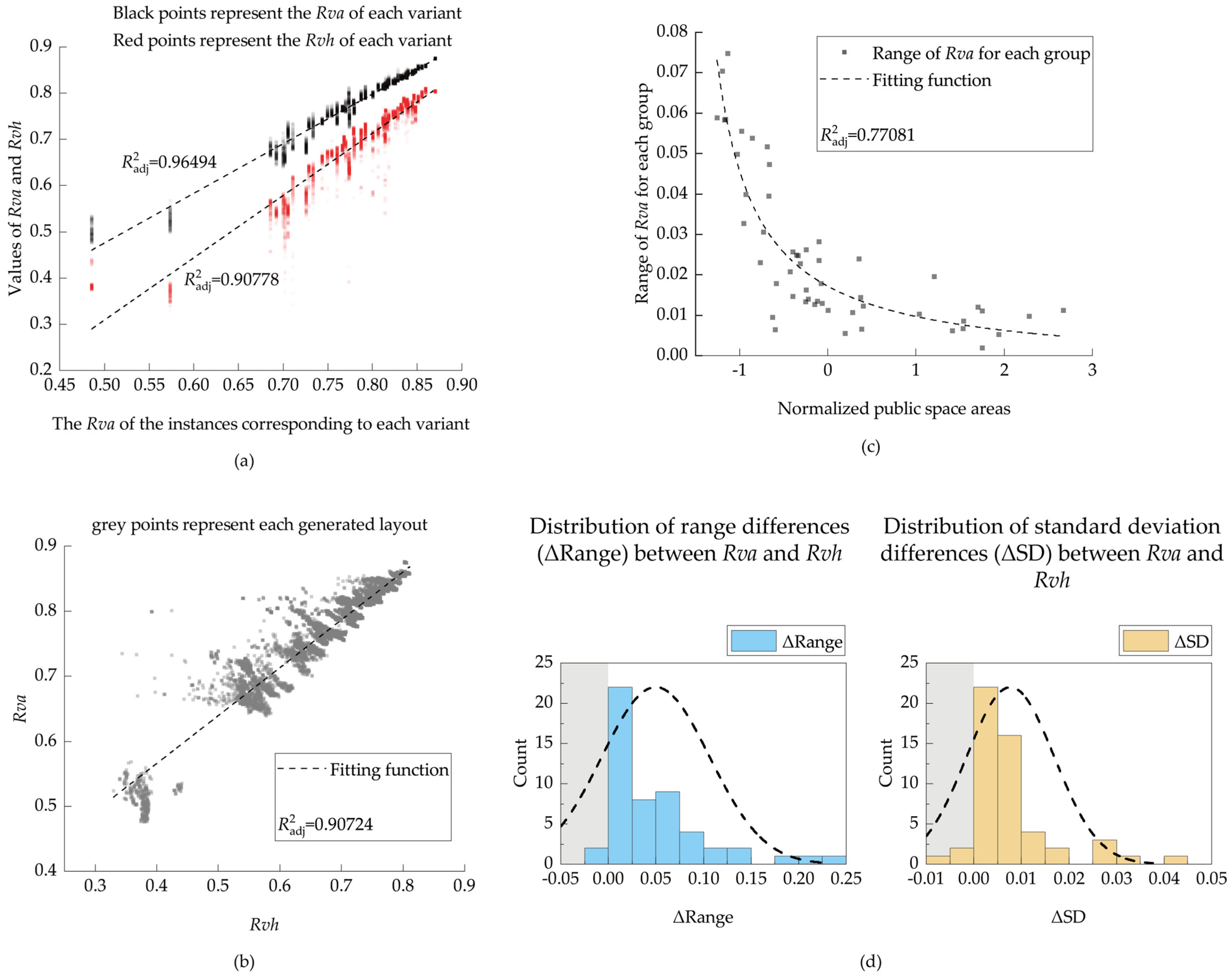
Using Python-based algorithmic iteration, 13,481 outputs were generated from the campus layouts of 53 collected primary and secondary schools. Instance No. 21 failed to produce viable variants due to algorithmic constraints, resulting in the final results being derived from 52 instances. All outputs were systematically numbered and grouped with their corresponding original instances. Finally, 52 groups were obtained. Visibility calculation maps for representative campus public spaces are provided in Appendix B, while arithmetic mean natural visibility ratios (Rva) are visualized in Figure 6a. In the figure, the horizontal axis represents the Rva values of the original instances within each group, while the vertical axis denotes the Rva values of their variants. Therefore, vertically aligned data points belong to the same group, with the color gradient (from light to dark) indicating the concentration of data points, thereby visualizing the frequency distribution of the Rva values in each group.
As illustrated in Figure 6a, the Rva values of the variants generally fluctuate around those of their corresponding instances, with values ranging from 0.49 to 0.88, being predominantly concentrated within the 0.7–0.85 interval. A linear regression analysis was performed on this dataset, yielding an R2 value of 0.965. This high coefficient of determination reflects the clustered distribution of the Rva values across the algorithm-generated variants, indicating limited variability in the safety outcomes that are due to the optimization of campus layouts. The statistical range of the Rva was calculated and visualized for each of the 52 groups, and these are shown in Figure 6c. The results indicate that the statistical ranges across all groups are primarily concentrated within the span of 0–0.06, accounting for approximately 8% of the total variability in Rva values. Furthermore, a rational regression analysis yielded an R2 value of 0.771, suggesting that, as the public space area increases, the maximum differences in Rva decrease. This implies that variations in building layouts have a diminishing impact on Rva as the size of the public space expands.

3.1.2. The Analysis of High-Occlusion Spaces

The harmonic mean of the natural visibility ratios (Rvh) for all instances and variants was calculated and is visualized in Figure 6a. A linear regression analysis yielded an R2 value of 0.908, which is lower than that of the Rva, indicating that the Rvh fluctuates even more. Further, for each of the 52 groups, the range and standard deviation (SD) of both the Rva and Rvh were calculated. The differences between these metrics were derived as follows:
R a n g e = R a n g e R v h R a n g e ( R v a )
S D = S D R v h S D ( R v a )
The distributions of ΔRange and ΔSD are visualized in Figure 6d. Most differences, both in the ranges and standard deviations, are positive, further supporting the heightened sensitivity of the Rvh to spatial feature variations. Linear regression analysis of the Rvh and Rva showed that the coefficient of determination R2 = 0.907 (Figure 6b). This value shows that the Rva can explain 90.7% of the variation in the Rvh, demonstrating a strong linear relationship between the two.
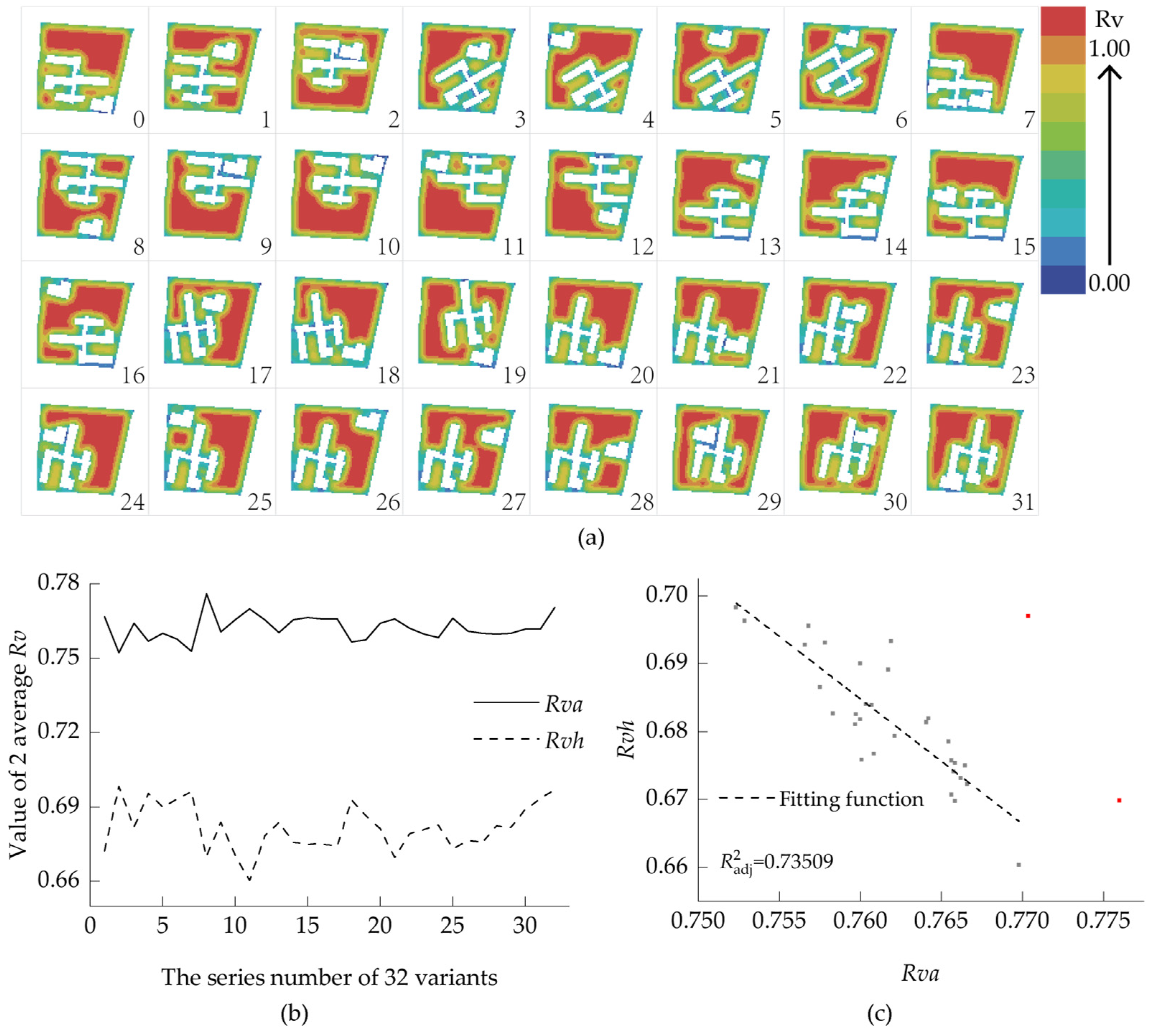
A systematic analysis demonstrates that spatial configurations differentially modulate visibility distribution characteristics. Compact layouts (smaller inter-building distances) increase the arithmetic mean visibility (Rva) by amplifying high-visibility zones, but simultaneously exacerbate the visibility disparity, a phenomenon captured by the harmonic mean visibility (Rvh) decline due to persistent low-visibility pockets (Figure 7). Conversely, dispersed layouts reduce visibility inequality (higher Rvh) at the cost of lower overall visibility averages (Rva). This trade-off originates from the mathematical duality of the metrics:
(1)
The Rva weights all spaces equally, favoring concentrated high-visibility clusters;
(2)
The Rvh penalizes low-visibility extremes, requiring homogeneous visibility distribution.
This inverse correlation is further supported by the LYTa and LYTh (ρ < 0, as Table 1). The two metrics employ the z-score normalization approach to map each school’s average natural visibility ratio into its corresponding group. The values of LYTa and LYTh reflect the relative performance of a school’s campus layout within its group. This confirms that optimizing one metric inevitably constrains the other, necessitating context-specific balancing in safety-focused design.
One school layout was randomly selected from the 53 campuses. Within the chosen campus, the positions and orientations of buildings were systematically adjusted to generate 32 variants (Figure 8a). This amount was chosen to ensure a sufficiently diverse set of building placements. During the adjustment process, the buildings were allowed to traverse a wide range of potential positions and orientations. Although some of the resulting variants did not yield reasonable outcomes, they were retained to capture the full spectrum of placements, ensuring that both typical and extreme scenarios were included. Variants that were too similar to others were, however, excluded. This approach helped verify the broader relationship between the campus layout and its security, even if some variants did not yield optimal results.
The calculated Rva and Rvh values for all variants (Figure 8b) reveal a systematic trade-off governed by their mathematical definitions. The Rva, quantifying the arithmetic mean visibility, ranges narrowly from 0.75234 to 0.77599 (Δ = 0.024, Figure 6c), while the Rvh—the harmonic mean—exhibits stronger sensitivity to localized occlusions due to its inherent penalty on low-visibility values (RvhRva holds universally).
This trade-off manifests in the extreme cases:
Variant 7 (highest Rva: 0.77599) employs a compact layout that maximizes overall visibility, but at the cost of concentrated low-visibility zones, suppressing its Rvh.
Variant 1 (highest Rvh: 0.69823) prioritizes visibility homogeneity through dispersion, avoiding severe occlusions but achieving a lower peak Rva.
The inverse ranking pattern (No. 7 leading in Rva but lagging in Rvh; No. 1 excelling in Rvh but not Rva) empirically validates the metrics’ antagonistic relationship. Meanwhile, the lowest Rvh values in Variants 7, 9, 10, and 20 directly reflect their higher proportions of spaces where visibility approaches zero, indicating that more high-occlusion spaces can be found in them.
As illustrated in Figure 8b, the solid line represents the Rva values, while the dashed line represents the Rvh values. The plot exhibits approximate axial symmetry across 32 variants, preliminarily suggesting a systematic inverse relationship between the two metrics. A subsequent linear regression analysis, conducted after excluding outliers with significant deviations, is presented in Figure 8c. The coefficient of determination (R2) was calculated to be 0.73509. Specifically, the Rva values are predominantly clustered within a narrow range of 0.752–0.770 (span: 0.018), whereas the Rvh displays a broader distribution between 0.660 and 0.698 (span: 0.038).
To further validate this relationship, Spearman correlation coefficients were calculated between the LYTa and LYTh values for these 32 variants (Table 2). These results align with the findings shown in Table 1, demonstrating a statistically significant negative correlation between LYTa and LYTh which mirrors the inverse relationship observed between Rva and Rvh. This directional consistency underscores a fundamental trade-off in safety-oriented design optimization: efforts to enhance overall visibility (reflected in elevated Rva) inadvertently amplify the prevalence of high-occlusion space (captured by lower Rvh). This occurs because the harmonic mean (Rvh) is inherently more sensitive to low-visibility extremes.
Overall, the harmonic mean of natural visibility ratios (Rvh) is more sensitive to disturbances caused by layout modifications compared to the arithmetic mean (Rva). When optimizing the public spaces of a given school, monitoring the Rvh enables the more efficient detection of high-occlusion spaces.

3.2. Public Space Form

3.2.1. The Correlation Between Public Space Density and Natural Visibility

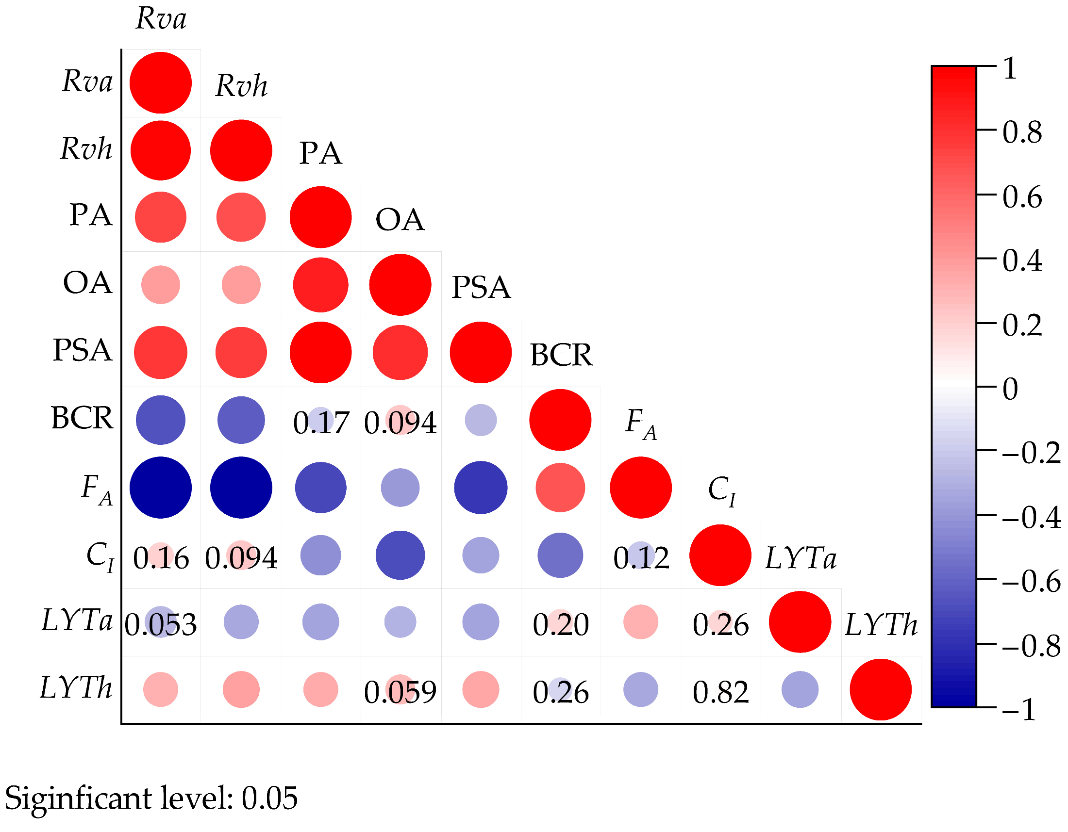
Among the 53 cases, Spearman correlation coefficients were computed between the natural visibility level (Rva and Rvh) and four attributes (Table 3): the property area (PA), public space area (PSA), obstacle area (OA), and building coverage rate (BCR). The analysis revealed a significant negative correlation between the BCR and Rva, which aligns with prior findings [19]. Notably, the PSA exhibited a strong positive correlation with the Rva, suggesting that the extent of public spaces on campus significantly influences the safety. The magnitude of the correlation coefficient for the PSA exceeded that of the BCR, indicating that the scale of public spaces has a more substantial impact on the Rva than the BCR. The PA and OA showed high positive correlations with the PSA, further supporting the positive relationship between the natural visibility level and these attributes. The Rvh, the harmonic mean of the natural visibility ratio, exhibits correlations with spatial configurations that are consistent with those of the Rva observed under the Spearman correlation analysis. This alignment confirms their complementary roles in holistic safety assessments.

3.2.2. The Correlation Between Public Space Shape and Natural Visibility

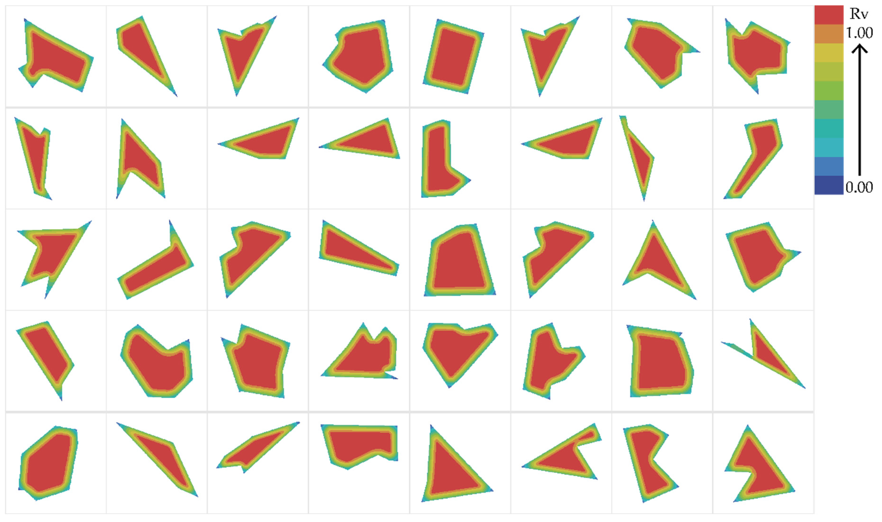
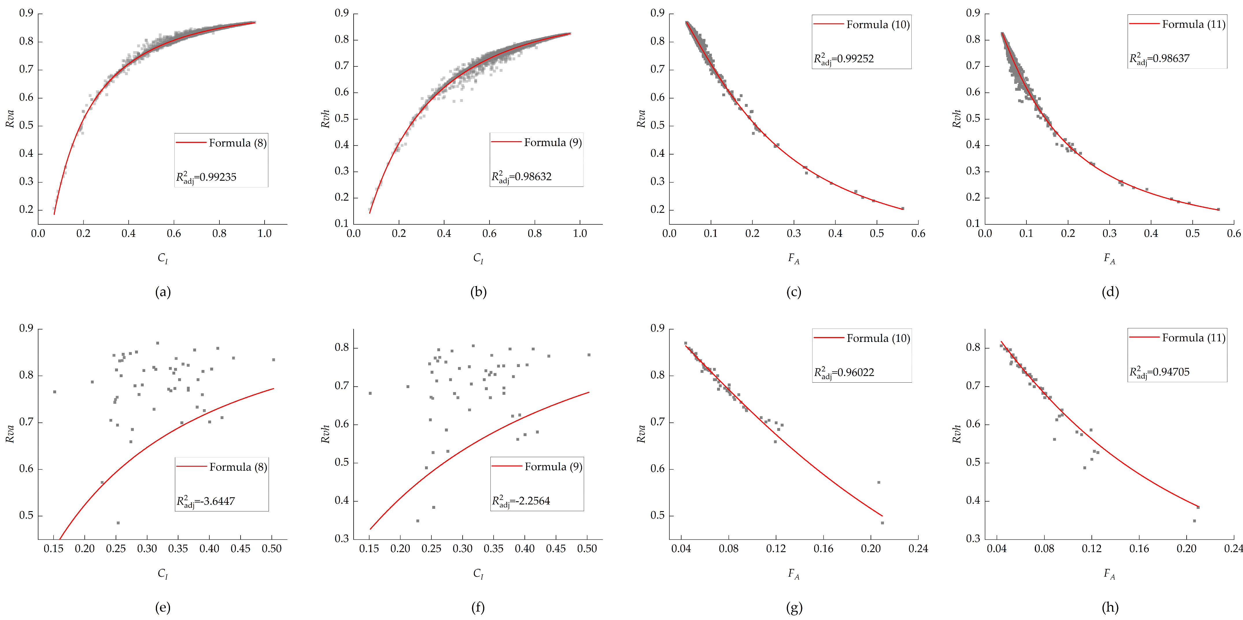
Excluding erroneous data, a total of 6770 polygon plots with equal areas were generated. The Rva, Rvh, CI, and FA for these were calculated. The CI was calculated followed Equation (3), and the value of μA was determined to be 1 in the calculation of the FA. Some of the calculation maps of these plots are presented in Appendix C. Scatter plots depicting the relationship between the Rva and the two indices are shown in Figure 9a and Figure 9c, respectively. The relationships between the Rvh and the two indices are shown in Figure 9b and Figure 9d, respectively. Since these plots have an equal area, the relationship between their CI and FA can be expressed as follows.
F A = 1 C I 2 π A μ A = k C I ,   k > 0
Therefore, in contrast to the CI, the smaller the FA, the more compact the plot, and the closer its shape is to a circle.
The fitting relation shown in Figure 9a reveals the correlation between the Rva of these random plots and the CI of their shapes, which and be expressed by Equation (8), with R2 = 0.992.
R v a = - 0.26309 + 7.66827 C I 1 + 7.0233 C I + 0.46108 C I 2 ,   C I > 0
The correlation between the Rvh and CI in Figure 9b is expressed by Equation (9), with R2 = 0.986.
R v h = 0.09685 + 3.85813 C I 1 + 3.20157 C I + 0.31824 C I 2 ,   C I > 0
The fitting relation presented in Figure 9c demonstrates the correlation between the Rva and the FA, which can be expressed by Equation (10), with R2=0.99252.
R v a = 0.97152 + 1.15162 F A 1 + 3.4845 F A + 15.7873 F A 2 ,   F A > 0
The correlation between the Rva and the FA in Figure 9d is expressed by Equation (11), with R2 = 0.986.
R v h = 1.00258 + 3.01696 F A 1 + 7.16029 F A + 39.26182 F A 2 ,   F A > 0
The results indicate that, for a given area, the Rva and Rvh are positively correlated with CI, and negatively correlated with FA. Since CI and FA are inversely proportional (Equation (7)), i.e., when the area is fixed, a more compact shape, which usually means that it is closer to a circle, of the plot is associated with higher visibility, which equals higher safety.
The same procedure was applied to the 53 cases to examine this result. The relation between the FA and the average natural visibility ratios (Rva and Rvh) is depicted in Figure 9g and Figure 9h, and the relation between the CI and the average natural visibility ratios is shown in Figure 9e and Figure 9f. The corresponding fitting equations, Equations (8)–(11), are also included in the plots, respectively.
It can be observed that the functional relationship described by Equations (10) and (11) demonstrates a strong fit with the instance data. In contrast, the distribution of points for the CI is relatively scattered, indicating a lack of significant correlation between the two. This means that the relation expressed by Equations (8) and (9) did not apply well to the instance data.

3.3. Integrated Impacts of Spatial Configurations on Natural Visibility

To determine both the collective influence of all spatial features on campus safety and their relative importance, a multiple linear regression analysis was conducted between these factors (morphological metrics) and the natural visibility level (Rva and Rvh). First, multicollinearity diagnostics were performed. Figure 10 presents the Spearman correlation matrix for all normalized independent variables, revealing strong collinearity among the PA, OA, and PSA. Notably, the PA is mathematically equivalent to PSA + OA, and both the PSA and OA can be derived from the PA and BSR. Given the redundancy among these variables and prior analyses demonstrating the PSA’s stronger correlation with Rva (Table 3), only the PSA was retained in the final model.
After excluding the PA and OA, the variance inflation factors (VIFs) for all remaining independent variables are presented in Table 4. The results indicate high multicollinearity between the building coverage rate (BCR) and the form area factor (FA). Table 5 shows the VIFs after further excluding the FA, revealing acceptable multicollinearity levels for subsequent multiple linear regression. However, considering that the FA significantly influences the safety performance, it was retained in a parallel regression model for comparative analysis. The results of the multiple regression analyses are presented in Table 6 and Table 7. All independent and dependent variables were normalized prior to regression.
Across the four regression models presented in Table 6 and Table 7, the spatial configurations (excluding building layout, represented by LYTa and LYTh) exhibit consistent directional effects on both the arithmetic mean (Rva) and harmonic mean (Rvh) of the natural visibility ratios. If a variable positively influences the Rva, it similarly enhances the Rvh, and vice versa. The LYTa and LYTh coefficients are inversely correlated in all models, reinforcing the inherent trade-off between holistic optimization and localized optimization in safety-focused design. The inclusion of the form area factor improves the models’ explanatory power (from Table 7 to Table 6, adjusted R2 increased). However, the role of other spatial features has decreased (elevated p-values in most variables).
In the model excluding the form area factor (FA) (Table 7), the PSA and CI show positive correlations with the natural visibility level, while the BCR displays a negative correlation—consistent with prior findings. The LYTa and LYTh exhibit the weakest associations, indicating a weak correlation between campus layout and safety. When the FA was incorporated, the LYTh gained relative importance in explaining safety outcomes. Although its coefficients for both the Rva and Rvh decrease, the LYTh ranks third in predictive significance for the Rvh—highlighting its role in mitigating high-occlusion spaces.

4. The Spatial Distribution of Student Activities for the Validation of the Natural Visibility Rate Results

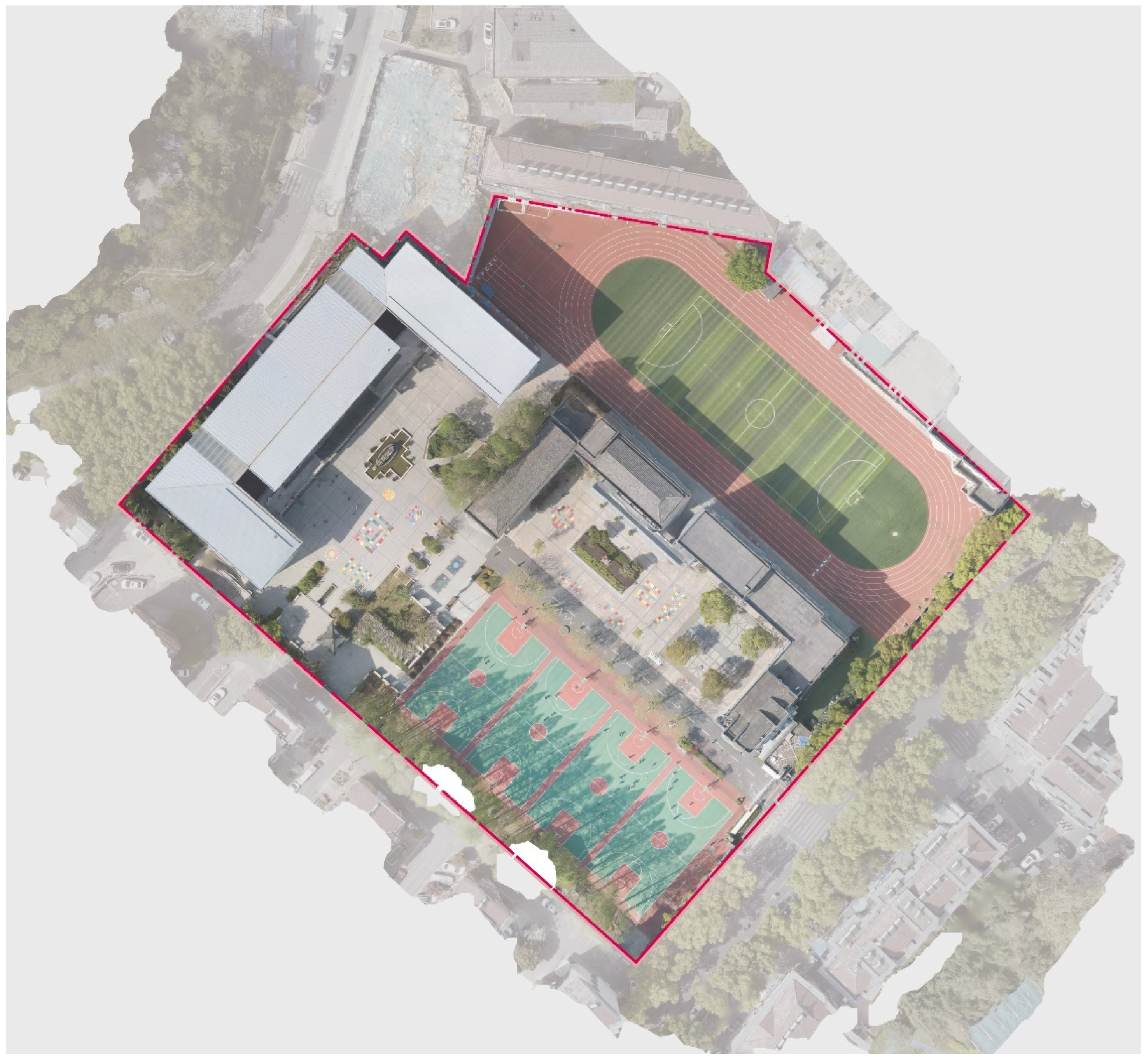
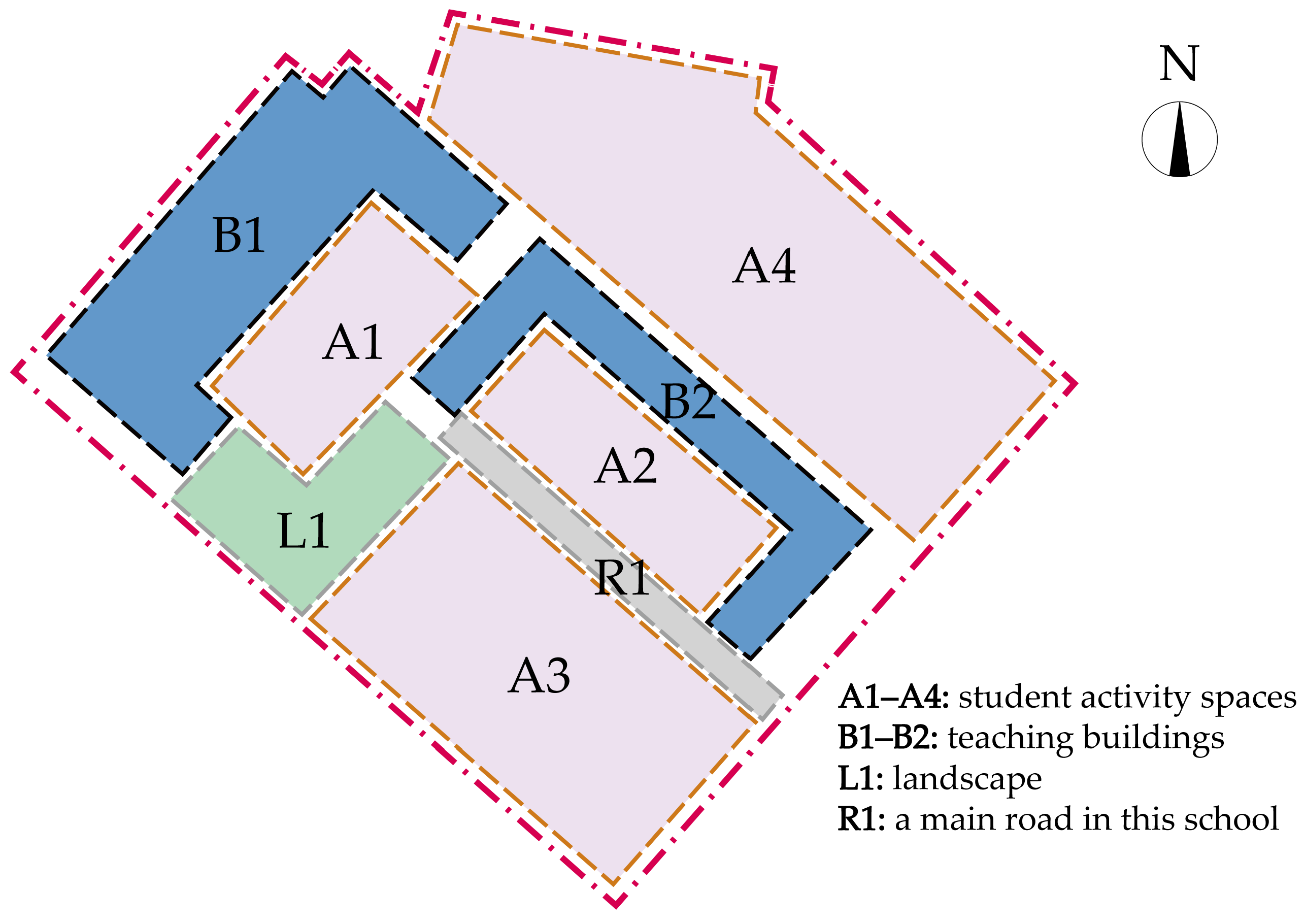
While computational modelling and statistical analytics elucidate quantitative correlations between spatial configurations and safety metrics, interrogating the behavioral mediation of these relationships remains imperative. To reconcile this empirical discrepancy, we conducted an empirical validation study at a representative urban primary school in Nanjing. The campus’s spatial organization, as documented in Appendix D, comprises two didactic structures (B1, B2) and functionally differentiated activity zones. Figure 11 illustrates the topological abstraction of the site plan through the following nodal elements:
  • A1–A4: designated student congregation zones during non-instructional intervals, with specialized programmatic allocations: A3: hardscape recreational facility with basketball courts; A4: synthetic turf playground integrating football field infrastructure;
  • R1: primary vehicular thoroughfare governed by temporal access restrictions (vehicle prohibition during education operations: 08:00–18:00);
  • L1: ecological buffer zone exhibiting minimal pedestrian interaction frequencies, serving primarily as visual relief space.
A one-week observation was conducted to analyze the student distribution patterns during recess periods. Drone aerial imagery was employed to capture real-time activity locations, which were processed into a student activity heatmap (Figure 12). Noon was not included in the data collection due to a scheduled lunch break. The Rv calculation map of the campus is also presented in Figure 12. Due to school management, with the aim of ensuring timely classroom returns and enhancing the management’s supervisory efficiency, student access to A4 (the playground) was limited during recess periods. Thus, A4 was excluded from both the Rv calculation map and the activity heatmap. This exclusion ensures that our spatial safety assessments reflect only areas where student activity actually occurs.
The Rva value consistently exceeds the Rvh due to its calculation methodology, which is not significantly influenced by extremely low values. As shown in Figure 13, the maximum Rv value exerts a positive impact on the Rva, enabling it to maintain balance even in the presence of low-value sub-regions through compensation from high-value regions. Conversely, the minimum Rv value directly constrains the lower limit of the Rvh. This calculation approach results in the reciprocal term of low-value sub-regions causing a sharp decline in the overall value. When the regional minimum Rv value falls below 0.2, nonlinear attenuation occurs in the Rvh, as exemplified by the rate of decline observed between A3 and A2.
As illustrated in Figure 12, there is a discernible correlation between student activity hotspots and areas with a higher natural visibility level, underscoring the critical role of spatial safety in shaping student behavior. Key observations include the following.
High-visibility zones: activity areas A2 and A3 exhibit the most high-visibility space (A2: Rva = 0.766, Rvh = 0.669; A3: Rva = 0.836, Rvh = 0.789), and correlate with peak student congregation. R1, although not a primary gathering zone, maintains high visibility (Rva = 0.899, Rvh = 0.876) and frequent interaction between A2 and A3. R1 and A3 belong to the high-visibility equalization zone with no significant obstacles, while A2 has an isolated blind zone.
Moderate visibility zones: A1, with a moderate visibility level (Rva = 0.669, Rvh = 0.612), attracts fewer students than A2 and A3.
Low-visibility zones: L1, a landscaped area obstructed by decorative structures and trees, shows minimal activity (Rva = 0.471, Rvh = 0.414), and also has poor natural surveillance. The spread of multiple blind spots requires a full-scale transformation.
The analysis of campus visibility demonstrates differentiated performances regarding the natural visibility across various areas, including R1 (main entrance area), A3, A2, and A1 (activity space), and L1 (landscape green space). From the high-visibility area R1 to the low-visibility area L1, the relative visibility arithmetic mean (Rva) exhibits a gradual decreasing trend, declining from 0.899 to 0.471, with an average reduction of approximately 0.107 per area. This linear attenuation reflects the systematic degradation of visual resources on campus, transitioning from the core area to the peripheral regions, which is potentially influenced by factors such as increasing building density gradients and rising vegetation coverage rates. In contrast, the relative visibility harmonic mean (Rvh) experiences a sharp decline from 0.876 to 0.414, representing a decrease of 52.7%, with notable inflection points observed in regions A2 (0.669) and L1 (0.414). This nonlinear change arises from the sensitivity amplification effect of the harmonic mean on low-visibility sub-regions. For instance, the minimum value of the Rv in region A2 is as low as 0.16, generating a six-fold amplification factor in the Rvh calculations, which leads to a significant drop in the overall values, while the Rva remains relatively stable at 0.766 due to the equilibrium characteristics of the arithmetic mean.
The spatio-temporal distribution of crowd activities exhibits dynamic correlations with visibility indices. High-Rva areas (R1-A2) attract substantial activity in the morning, whereas the activity shifts to Rvh-sensitive areas (A3/L1) in the afternoon. The solid wall interface of teaching building B2 (with a minimum Rv value of 0.15) coincides with peak student density in the afternoon, creating a risk overlap of “high activity—low visibility”. The mismatch between students’ safety expectations and visibility indicators highlights the complexity of environmental perception—despite the theoretical visual advantages in high-Rva areas (e.g., the main entrance area R1, Rva = 0.899), “Transparency Fatigue” induced by their linear layout may diminish the actual sense of security. During peak activity periods in the afternoon, students congregate in A2 (Rva = 0.669) and A3 (Rvh = 0.789), indicating that psychological safety relies more on controllable visibility—namely, the ability to actively adjust one’s visible range rather than being passively exposed to full-domain monitoring. Consequently, “Rva-oriented design” on campus should not overly emphasize visual order but instead mitigate Rvh attenuation and avoid excessive exposure that could induce psychological discomfort. Natural visibility compensation at the architectural design level can be achieved through composite structures, such as the use of cantilever landscape platforms for field-of-view compensation, or addressing insufficient visibility in Rvh-sensitive areas through monitoring equipment.
In summary, the difference in sensitivity between the Rva and Rvh fundamentally represents the complementarity of assessment perspectives: the Rva objectively quantifies the total amount of visible resources, while the Rvh precisely identifies local defects. Through spatial diagnosis and transformation driven by extreme value data, systematic improvements can be realized, progressing from macroscopic coverage to microscopic optimization, ultimately constructing a resilient visual network system to enhance campus security [70].

5. Discussion

5.1. Building Layout and Campus Safety

The analysis of 53 campuses with varying building layouts revealed that the impact of these configuration on campus safety is statistically negligible. As demonstrated in Figure 6c and Figure 8b, the Rva remains confined to a narrow range around the original value, indicating limited variability despite adjustments to the layout. Regression analyses (Table 6 and Table 7) further corroborate this: both the LYTa and LYTh exhibit minimal impacts on the arithmetic mean natural visibility ratio (Rva), as evidenced by their small coefficients and statistically insignificant p-values in the regression model. This signifies a minimal influence of the layout on safety outcomes. However, although minor, fluctuations in the Rva and Rvh that were observed across different configurations suggest that changes in building positioning and orientation can influence the natural visibility level in public spaces, which may theoretically affect campus safety. Nevertheless, the extent of any safety changes does not depend solely on specific modifications to building layouts but rather on how the spatial characteristics and form of public spaces are altered. When buildings are designed more compactly, typically through closer proximity or reduced interval spaces between structures, the overall campus safety tends to improve. From a holistic perspective, it is more advantageous to organize campus public spaces into fewer, more cohesive, and more secure areas rather than dispersing them into numerous smaller activity zones. Nonetheless, this ideal configuration is not always attainable in practical design scenarios.
In contrast, the scale of public space has a more substantial impact on campus safety. As indicated by the Spearman correlation coefficients (Table 3), the area of public spaces exhibits a stronger correlation with the natural visibility level (Rva and Rvh) compared to other indices, underscoring its direct influence on campus safety. This also elucidates the negative relationship that was observed between the building coverage rate and the Rva [19]. In general design practice, increasing the building coverage rate often results in reduced outdoor spaces, leading to fewer or narrower activity areas for students and more parts of the campus becoming sheltered by buildings. Consequently, less space remains under adequate natural surveillance.
The relationship between the building area and natural visibility level (Rva and Rvh) exhibits a comparable pattern. Design codes and regulations dictate that the configuration of activity spaces and classrooms is primarily determined by student numbers, thereby establishing a quantitative correlation among the public space area, building area, and building coverage rate. Schools situated on larger plots of land tend to maintain more expansive public spaces, thus facilitating safer campuses. Furthermore, the scale of public space significantly influences the extent to which campus safety can be optimized through adjustments to the building layout. In our sample, schools with relatively smaller public spaces experienced greater fluctuations in their natural visibility level when their layouts were modified. In most practical scenarios, schools with limited land for construction must allocate areas for playgrounds and sports fields, making it challenging to rearrange the position and orientation of buildings. Additionally, due to service radius constraints, small-scale primary and secondary schools are less common in urban areas, particularly in eastern China, and are underrepresented in our selected cases. Consequently, adjusting the building layout typically does not significantly enhance the overall campus safety. This reinforces the notion that campus safety is more strongly influenced by the scale of public space than by the building configuration. Ultimately, the scope of human vision remains unaffected by changes in spatial form; once the total area of public space is established, the potential for natural surveillance within that space becomes relatively fixed.

5.2. Public Space Morphology and Campus Safety

For architects, while it is typically impossible to significantly optimize campus safety through adjustments in the configurations of buildings alone, modifying the morphology of public spaces can indeed improve their safety to some extent. As shown, the compactness index is strongly correlated with the average natural visibility ratio (arithmetic mean), suggesting that spaces with shapes closer to a circle are considered safer. More specifically, the CI evaluates the relationship between the perimeter and area of a shape, meaning that, for a given area, a shape with a smaller perimeter is closer to a circular form. This implies that, in the design process, to enhance the safety of school public spaces, it is preferable to simplify their boundaries, minimizing protrusions and concave volumes.
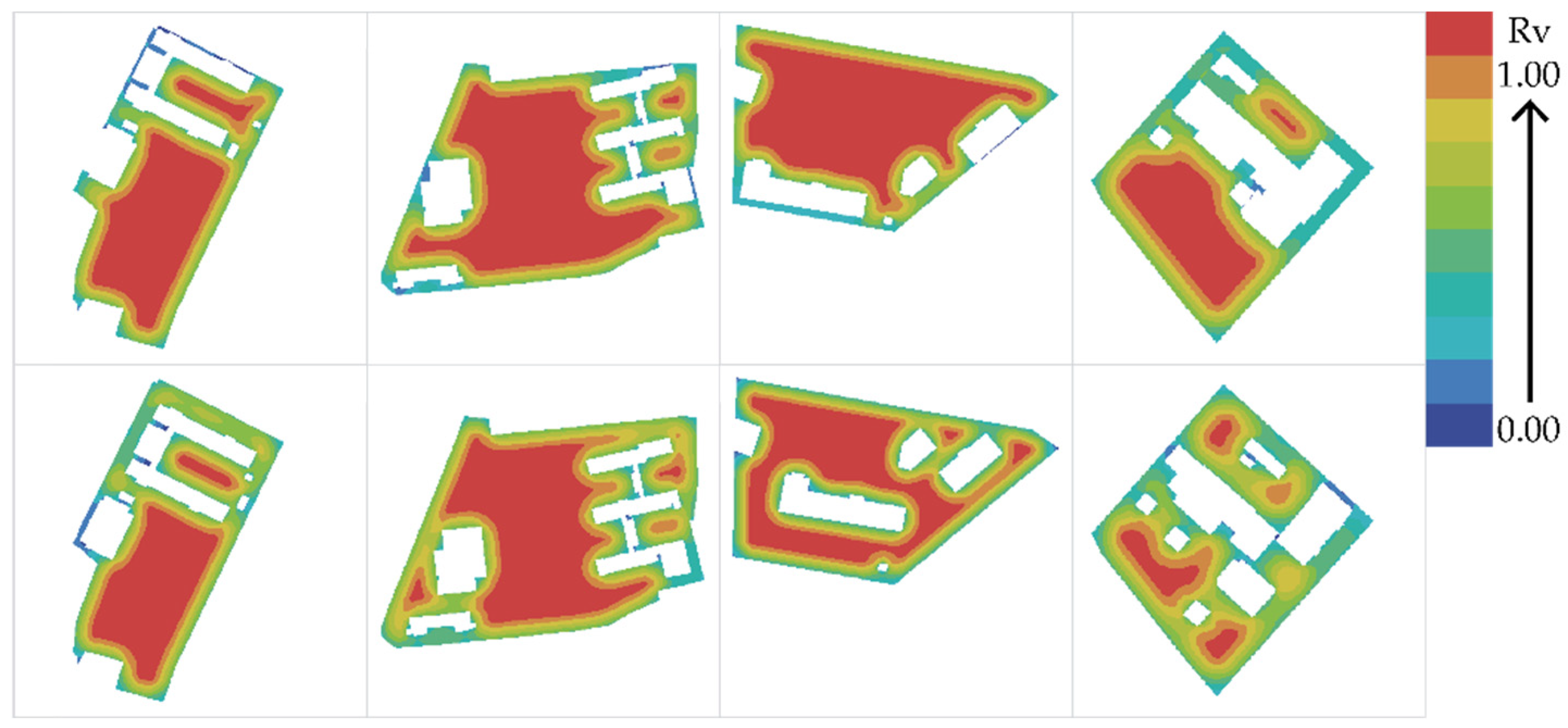
The form area factor (FA) links the spatial form to its safety, and maintains a relationship with both the compactness index (CI) and the shape factor. If the area is determined, the FA serves a similar function to the CI. But common architectural design strategies, such as the combination and subtraction of volumes, do not always preserve a constant area. Moreover, making a shape more regular or compact does not necessarily enhance the resulting safety. Figure 14 illustrates several typical spatial organization approaches. The adjustment from Case 1 to Case 2 is representative, demonstrating how adjusting the shape of a space can enhance its safety. From Case 2 to Case 3, although the combination of spaces led to a more complex form and a reduction in CI, the safety actually improved. In contrast, the change from Case 1 to Case 4 shows that simplifying the shape of the public space by subtracting from its volume resulted in a decrease in safety. These examples highlight that both the scale and shape of a space are crucial considerations in safety-oriented design.
The form area factor can be considered a simplified representation of the shape factor. The shape factor quantifies the intricacy of building volumes and is widely utilized in calculations pertaining to building thermal performance and energy consumption. In the context of school design, outdoor public space is defined as the residual area after accounting for building footprints. Therefore, a more complex architectural volume inherently increases the complexity of the surrounding public space. According to this study’s findings, controlling the shapes of buildings is crucial for both building performance and campus safety. This relationship between form and safety elucidates why modifications to building configurations can result in subtle changes in the resulting Rva. The Rva measures the overall safety of all target points within a space, with the shape of the public space being continuously altered during the adjustment process. Although the total number of target points remains relatively constant, the Rv value for each individual point fluctuates. As buildings are reconfigured and brought closer together, the area of high-occlusion spaces enclosed by buildings decreases, while the perimeter of these spaces changes less significantly. Consequently, their form area factor (FA) increases, leading to a reduction in overall safety. When the average natural visibility ratio is computed using the arithmetic mean, the Rva increases due to the reduction in the total area of high-occlusion spaces. However, because these spaces become less secure, the Rvh, calculated using the harmonic mean, decreases.

5.3. Reconciling Natural Visibility and Safety in Campus Design

In campus spatial safety design, the dialectical relationship between localized optimization and systemic equilibrium unveils fundamental challenges in architectural configuration. When designers seek to enhance the natural surveillance efficacy in specific zones through concentrated building masses, such interventions often trigger spatial performance redistribution—the visual accessibility advantages created by high-density layouts may engender line-of-sight discontinuities in adjacent transitional areas, forming novel security vulnerabilities. The spatiotemporal divergence revealed in the thermal maps—morning activity aggregation (Figure 12a) versus afternoon diffusion (Figure 12b)—confirms the limitations of singular spatial strategies. While compact configurations strengthen directional crowd control during morning peak periods, they prove inadequate in addressing omnidirectional visibility demands during afternoon free-activity intervals. This temporal-spatial heterogeneity necessitates transcending static performance optimization in favor of dynamic responsive mechanisms.
The Rv calculation map (Figure 12c), with its high-intensity red zones marking visual surveillance efficacy peaks, demonstrates the spatial transfer law of safety performance through edge transition fractures. Each localized visibility enhancement potentially stimulates surveillance blind spot proliferation in neighboring areas, essentially manifesting the principle of performance conservation within finite spatial resources. Under fixed-site constraints, visibility improvement cannot exist as an independent variable but must engage in dynamic negotiation with functional organization and circulation efficiency.
This trade-off phenomenon compels designers to make paradigmatic choices: either create high-intensity security cores and accept peripheral surveillance degradation, or adopt dispersed layouts and sacrifice peak visibility for balanced baseline safety enhancement. Contemporary campus design is transitioning from mechanical functional zoning to resilient space organizing.
Through the synergistic operation of adjustable interfaces (e.g., movable partitions, intelligent shading systems) and hybrid functional modules (compound corridors, polyvalent courtyards), the autonomous temporal adaptation of spatial performance can be achieved.
After all, based on our simulation results and case study observations, we recommend that the main activity spaces of school maintains an Rva and Rvh of no less than 0.5. For areas that are fully enclosed (or nearly so), an FA of no more than 0.2 is suggested to balance the building layout with safety considerations. When evaluating all public spaces on a campus as a whole, we recommend that the overall FA should not exceed 0.2.

5.4. Digital Technology for Solving Architectural Problems

Digital technology plays an indispensable role in this research. For instance, comparing different campus layouts is inherently challenging due to the significant variability in architectural forms within schools, making it difficult to identify two cases with distinct layout types but other similar conditions. However, algorithms can effectively control for extraneous variables, enabling the exploration of all feasible and hypothetical design proposals during the school design phase. This process ultimately reveals patterns and relationships that would otherwise remain obscured. Additionally, certain issues can be studied more efficiently using this approach. For example, as illustrated in Figure 9a,c, the compactness index (CI) is not entirely independent of the relative visibility (Rva); rather, it must be considered under the condition that the area of public space remains constant. The algorithm not only simulated this scenario but also expanded the sample size, thereby enhancing the reliability and robustness of the results.
Programming offers a distinct advantage in generating statistically significant results, which assist in making qualitative judgments regarding architectural issues. Although this research did not conclusively establish a direct and strict correlation between a smaller form area factor (FA) and higher security, the morphological factors influencing safety are complex and difficult to define precisely. Therefore, the probabilistic phenomena produced by the program remain meaningful. As shown in Figure 14, when optimizing Case 4, it is suggested to simplify the shape to transform it into Case 2 or to add a block to achieve Case 1. Digital technology excels in efficiently traversing a large number of possible solutions, making it far more effective in obtaining such statistical results.

6. Conclusions

This study establishes a computational framework that reconciles localized visibility optimization with systemic spatial equilibrium in campus safety design, and is grounded in the natural visibility principles of crime prevention through environmental design (CPTED). By employing Python-driven hill-climbing algorithms to iteratively generate and refine architectural variants, combined with space syntax-based visibility analysis, we demonstrate the inherent tension between micro-scale geometric interventions and the balance of macro-scale surveillance. The methodology reveals that localized enhancements in visual permeability—achieved through simplified building footprints and regularized public space geometries—invariably reconfigure systemic visibility patterns, often at the expense of peripheral monitoring efficacy.
The space syntax analysis of axial integration and isovist characteristics across algorithmically generated layouts confirmed a fundamental design paradox: concentrated visibility improvements in high-activity zones (e.g., courtyards, plazas) systematically induce fragmented surveillance blind spots in transitional areas. This phenomenon adheres to a conservation principle of visibility resources, where geometric optimization in one spatial domain necessitates compensatory adjustments elsewhere. This research identifies regular quadrilateral and circular morphologies as optimal mediators, balancing focal surveillance intensity with distributed visual connectivity.
The introduced form area factor (FA) metric, combined shape factor, and compactness index, in quantifying shapes, were strongly positively correlated with campus safety, providing a new tool for safety-oriented design. Our findings challenge conventional safety design paradigms by demonstrating that holistic security emerges not from maximizing isolated visibility metrics, but from strategically calibrating visibility gradients across functionally differentiated zones. For constrained urban campuses, the vertical integration of layered visibility corridors and the intelligent consolidation of fragmented spaces prove critical in maintaining systemic equilibrium.
This methodology advances CPTED theory by bridging natural visibility principles with computational spatial analysis, offering a reproducible framework for evidence-based campus design. Future research directions include integrating real-time crowd dynamics modeling with adaptive visibility systems, potentially revolutionizing safety design through responsive architectural interfaces. This study ultimately positions campus safety as a dynamic spatial construct, demanding continuous negotiation between localized interventions and global performance thresholds.

Author Contributions

Conceptualization, F.L. and H.Z.; methodology, F.L. and H.Z.; software, H.Z. and S.L.; validation, J.X. and Y.T.; formal analysis, H.Z.; investigation, H.Z. and Y.T.; resources, F.L. and H.Z.; data curation, H.Z.; writing—original draft preparation, H.Z.; writing—review and editing, F.L., J.X., Y.T. and S.L.; visualization, H.Z.; supervision, F.L., J.X. and S.L.; project administration, F.L.; funding acquisition, F.L. and H.Z. All authors have read and agreed to the published version of the manuscript.

Funding

This research was supported by the National Natural Science Foundation of China (No. 52108014) and the Postgraduate Research & Practice Innovation Program of Jiangsu Province (2025).

Data Availability Statement

The raw data supporting the conclusions of this article will be made available by the authors on request.

Acknowledgments

We gratefully acknowledge the assistance of graduate student Chenxi Yang in conducting the empirical validation study during the one-week student activity observations.

Conflicts of Interest

The authors declare no conflicts of interest.

Appendix A

Figure A1. The locations of the 53 primary and secondary schools: (a) the locations of the sampled schools, (b) the cities where a portion of sampled school located, (c) the cities where a portion of sampled school located.
Buildings 15 01472 g0a1

Appendix B

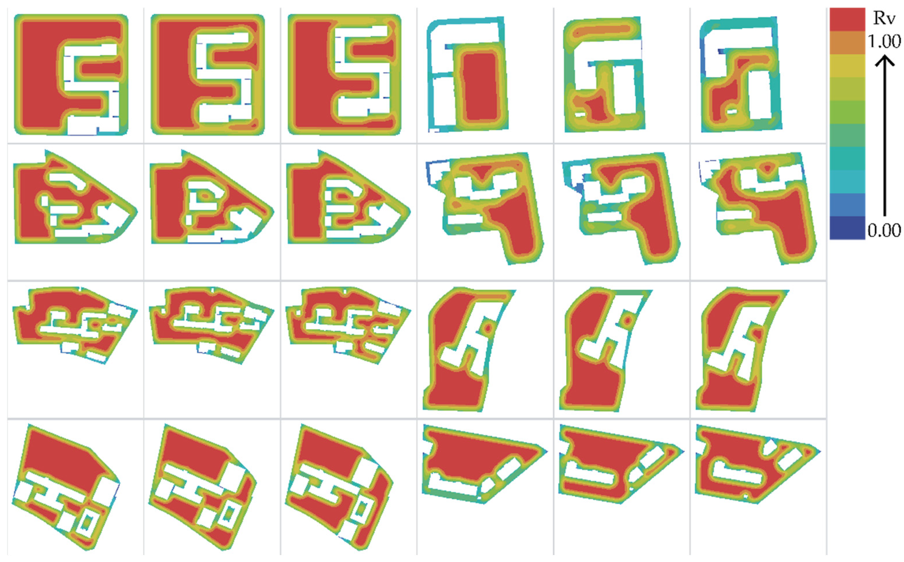
Figure A2. Part of the calculation results of campus public space Rv under the algorithm.
Buildings 15 01472 g0a2

Appendix C

Figure A3. Partial calculation map of random parcels natural visibility ratio.
Buildings 15 01472 g0a3

Appendix D

Figure A4. Site plan of the sampled primary school in Nanjing.
Buildings 15 01472 g0a4

References

  1. Cornell, D.G.; Mayer, M.J.; Sulkowski, M.L. History and Future of School Safety Research. Sch. Psychol. Rev. 2020, 50, 143–157. [Google Scholar] [CrossRef]
  2. Addington, L.A. Cops and Cameras: Public School Security as a Policy Response to Columbine. Am. Behav. Sci. 2009, 52, 1426–1446. [Google Scholar] [CrossRef]
  3. Wood, S.N. Mapping School Geographies: Teaching and Learning in Unsafe Places. J. Sch. Violence 2005, 4, 71–89. [Google Scholar] [CrossRef]
  4. Ministry of Education of the People’s Republic of China. Fortifying Campus Safety with a Sense of Responsibility That Is “Always on Our Minds”. China Education News, 30 January 2024. [Google Scholar]
  5. Gooren, J. The Logic of CPTED for Public Space or the Social Potential of Physical Security. Crime Law Soc. Change 2023, 79, 417–436. [Google Scholar] [CrossRef]
  6. Perumean-Chaney, S.E.; Sutton, L.M. Students and Perceived School Safety: The Impact of School Security Measures. Am. J. Crim. Justice 2013, 38, 570–588. [Google Scholar] [CrossRef]
  7. Lamoreaux, D.; Sulkowski, M.L. An Alternative to Fortified Schools: Using Crime Prevention Through Environmental Design (CPTED) to Balance Student Safety and Psychological Well-Being. Psychol. Sch. 2020, 57, 152–165. [Google Scholar] [CrossRef]
  8. Sohn, D.-W. Residential Crimes and Neighbourhood Built Environment: Assessing the Effectiveness of Crime Prevention through Environmental Design (CPTED). Cities 2016, 52, 86–93. [Google Scholar] [CrossRef]
  9. Hunter, J.; Garius, L.; Hamilton, P.; Wahidin, A. Who Steals from Shops, and Why? A Case Study of Prolific Shop Theft Offenders. In Retail Crime; Crime Prevention and Security Management; Palgrave Macmillan: Cham, Switzerland, 2018; pp. 71–97. [Google Scholar] [CrossRef]
  10. Seo, S.Y.; Lee, K.H. Effects of Changes in Neighbourhood Environment Due to the CPTED Project on Residents’ Social Activities and Sense of Community: A Case Study on the Cheonan Safe Village Project in Korea. Int. J. Urban Sci. 2017, 21, 326–343. [Google Scholar] [CrossRef]
  11. Son, D.; Im, B.; Her, J.; Kim, S.-N. Effects of CPTED Principles on Intention to Burgle in High-Density Low-Rise Residential Areas of South Korea: A Virtual Reality Experiment. Sage Open 2024, 14, 21582440241296723. [Google Scholar] [CrossRef]
  12. Bradshaw, C.P.; Milam, A.J.; Furr-Holden, C.D.M.; Lindstrom Johnson, S. The School Assessment for Environmental Typology (SAfETy): An Observational Measure of the School Environment. Am. J. Community Psychol. 2015, 56, 280–292. [Google Scholar] [CrossRef]
  13. Vagi, K.J.; Stevens, M.R.; Simon, T.R.; Basile, K.C.; Carter, S.P.; Carter, S.L. Crime Prevention Through Environmental Design (CPTED) Characteristics Associated With Violence and Safety in Middle Schools. J. Sch. Health 2018, 88, 296–305. [Google Scholar] [CrossRef] [PubMed]
  14. Schneider, R.H.; Kitchen, T.; Schneider, R.H. Planning for Crime Prevention; Routledge: London, UK, 2002. [Google Scholar]
  15. Liu, C.; Zhang, Y.; Zhang, J. Optimal Design for the Elementary School Campus Space Based on CPTED Theory. Urban. Archit. 2018, 2, 55–58. [Google Scholar]
  16. Ju, C. Research on the Status of Rural Idle Schools and Building Reform in Weihai. Master’s Thesis, China Central Academy of Fine Arts, Beijing, China, 2020. [Google Scholar]
  17. Hu, R. Based on CPTED Theory, the Space Design of Dormitory Area in Primary and Middle Schools Against Bullying. Master’s Thesis, University of Jinan, Jinan, China, 2021. [Google Scholar]
  18. Fujii, T.; Fujiwara, Y.; Oikawa, K. A Quantitative Analysis of Natural Surveillance at Elementary Schools-Evaluation Method Based on Perspectives from Both Outside Visibility and Visibility from Inside Buildings. J. Asian Archit. Build. Eng. 2013, 12, 17–23. [Google Scholar] [CrossRef]
  19. Liu, F.; Hu, Z.; Tang, Y.; Xie, J. Natural Visibility Measurement of Public Space in Primary and Secondary Schools. Sci. Technol. Eng. 2019, 19, 342–349. [Google Scholar]
  20. Li, C. Optimization Design of Xiamen Bindong Primary School Based on Natural Visibility Rate Simulation of Public Space. Fujian Constr. Sci. Technol. 2024, 13–15. [Google Scholar]
  21. Cozens, T.P. Love A Review and Current Status of Crime Prevention through Environmental Design (CPTED) (Article). J. Plan. Lit. 2015, 30, 393–412. [Google Scholar] [CrossRef]
  22. Ekblom, P. Redesigning the Language and Concepts of Crime Prevention through Environmental Design. In Proceedings of the Criminology and Criminal Justice, Ajman, United Arab Emirates, 11–14 March 2013. [Google Scholar]
  23. Ekblom, P. Deconstructing CPTED… and Reconstructing It for Practice, Knowledge Management and Research. Eur. J. Crim. Policy Res. 2011, 17, 7–28. [Google Scholar] [CrossRef]
  24. Braggs, D. Webcams in Classrooms: How Far Is Too Far. JL Educ. 2004, 33, 275. [Google Scholar]
  25. Altenburger, E.; Russell, L. Safety and Exposure in Transparent School Interiors: Patterned User Perceptions of Glass. J. Inter. Des. 2023, 48, 223–241. [Google Scholar] [CrossRef]
  26. Yin, X. The Research on the Investigation and Countermeasures of Violent Crimes on Campus in Recent Years. J. Xingtai Polytech. Coll. 2023, 40, 69–72. [Google Scholar]
  27. Voight, A.; Nation, M. Practices for Improving Secondary School Climate: A Systematic Review of the Research Literature. Am. J. Community Psychol. 2016, 58, 174–191. [Google Scholar] [CrossRef] [PubMed]
  28. Altenburger, E.; Wellenreiter, B.R. Where to Hang Out: Interplay Between School Building Characteristics, Authority Structures, and School Micro-Climates. Child. Youth Environ. 2021, 31, 1–33. [Google Scholar] [CrossRef]
  29. Kwon, C. Architectural Typologies of School Outdoor Spaces by Cases Study of the School Design Guidelines. Int. J. Sustain. Build. Technol. Urban Dev. 2022, 13, 231–240. [Google Scholar] [CrossRef]
  30. Shach-Pinsly, D. Measuring Security in the Built Environment: Evaluating Urban Vulnerability in a Human-Scale Urban Form. Landsc. Urban Plan. 2019, 191, 103412. [Google Scholar] [CrossRef]
  31. Oliveira, V. Urban Morphology: An Introduction to the Study of the Physical Form of Cities; Springer International Publishing: Cham, Switzerland, 2016; ISBN 3-319-32083-1. [Google Scholar]
  32. Kropf, K. The Handbook of Urban Morphology; John Wiley & Sons: Hoboken, NJ, USA, 2017; ISBN 1-118-74782-8. [Google Scholar]
  33. Ye, Y.; Li, D.; Liu, X. How Block Density and Typology Affect Urban Vitality: An Exploratory Analysis in Shenzhen, China. Urban Geogr. 2018, 39, 631–652. [Google Scholar] [CrossRef]
  34. Oliveira, V. Morpho: A Methodology for Assessing Urban Form. Urban Morphol. 2013, 17, 21–33. [Google Scholar] [CrossRef]
  35. Makki, M.; Showkatbakhsh, M.; Tabony, A.; Weinstock, M. Evolutionary Algorithms for Generating Urban Morphology: Variations and Multiple Objectives. Int. J. Archit. Comput. 2019, 17, 5–35. [Google Scholar] [CrossRef]
  36. Kachroo, P.; Bhatia, S.Y.; Patil, G.R. Computational Geometry-Based Kinematic Morphology for Urban Growth. Transp. Dev. Econ. 2024, 10, 11. [Google Scholar] [CrossRef]
  37. Desyllas, J.; Connoly, P.; Hebbert, F. Modelling Natural Surveillance. Environ. Plan. B Urban Anal. City Sci. 2003, 30, 643–655. [Google Scholar] [CrossRef]
  38. Rahimbakhsh, H.; Kohansal, M.E.; Tarkashvand, A.; Faizi, M.; Rahbar, M. Multi-Objective Optimization of Natural Surveillance and Privacy in Early Design Stages Utilizing NSGA-II. Autom. Constr. 2022, 143, 104547. [Google Scholar] [CrossRef]
  39. Hillier, B.; Leaman, A.; Stansall, P.; Bedford, M. Space Syntax. Environ. Plan. B Plan. Des. 1976, 3, 147–185. [Google Scholar] [CrossRef]
  40. Hillier, B. Space Is the Machine: A Configurational Theory of Architecture; Space Syntax: London, UK, 2007. [Google Scholar]
  41. Fu, J.-M.; Tang, Y.-F.; Zeng, Y.-K.; Feng, L.-Y.; Wu, Z.-G. Sustainable Historic Districts: Vitality Analysis and Optimization Based on Space Syntax. Buildings 2025, 15, 657. [Google Scholar] [CrossRef]
  42. Karimi, K. A Configurational Approach to Analytical Urban Design: ‘Space Syntax’ Methodology. Urban Des. Int. 2012, 17, 297–318. [Google Scholar] [CrossRef]
  43. Cutumisu, N.; Spence, J.C. Exploring Associations Between Urban Environments and Children’s Physical Activity: Making the Case for Space Syntax. J. Sci. Med. Sport 2009, 12, 537–538. [Google Scholar] [CrossRef] [PubMed]
  44. Zhang, B.; Li, B. From Knowledge Encoding to Procedural Generation for Early-Stage Layout Design: A Case of Linear Shopping Centres. Front. Archit. Res. 2025, 14, 282–294. [Google Scholar] [CrossRef]
  45. Safizadeh, M.; Hedayati Marzbali, M.; Abdullah, A.; Maghsoodi Tilaki, M.J. Integrating Space Syntax and CPTED in Assessing Outdoor Physical Activity. Geogr. Res. 2024, 62, 309–330. [Google Scholar] [CrossRef]
  46. Nubani, L.; Wineman, J. The Role of Space Syntax in Identifying the Relationship between Space and Crime. In Proceedings of the Proceedings of the 5th Space Syntax Symposium on Space Syntax, Delft, The Netherlands, 13–17 June 2005; pp. 13–17. [Google Scholar]
  47. Arghyani, M. Evaluating the Effect of Physical Components on the Promotion of the Sense of Security in Educational Spaces from the Perspective of Students; Case Study: High Schools of Bojnourd. Arman. Archit. Urban Dev. 2020, 13, 1–16. [Google Scholar] [CrossRef]
  48. GB 50099—2011; Code for Design of School. Ministry of Housing and Urban-Rural Development of the People’s Republic of China China Architecture Publishing & Media Press: Beijing, China, 2010.
  49. Crowe, T.D. Crime Prevention Through Environmental Design; Butterworth-Heinemann: Oxford, UK, 1991. [Google Scholar]
  50. Armitage, R.; Monchuk, L.; Rogerson, M. It Looks Good, but What Is It Like to Live There? Exploring the Impact of Innovative Housing Design on Crime. Eur. J. Crim. Policy Res. 2011, 17, 29–54. [Google Scholar] [CrossRef]
  51. Byun, G.; Ha, M. Factors of a Surveillance Environment That Affect Burglaries in Commercial Districts. J. Asian Archit. Build. Eng. 2016, 15, 73–80. [Google Scholar] [CrossRef]
  52. Jong, M.D.; Wagenaar, W.A.; Wolters, G.; Verstijnen, I.M. Familiar Face Recognition as a Function of Distance and Illumination: A Practical Tool for Use in the Courtroom. Psychol. Crime Law 2005, 11, 87–97. [Google Scholar] [CrossRef]
  53. Loukaitou-Sideris, A.; Liggett, R.; Iseki, H.; Thurlow, W. Measuring the Effects of Built Environment on Bus Stop Crime. Environ. Plan. B Urban Anal. City Sci. 2001, 28, 255–280. [Google Scholar] [CrossRef]
  54. GB 50352—2019; Uniform Standard for Design of Civil Buildings. Ministry of Housing and Urban-Rural Development of the People’s Republic of China China Architecture Publishing & Media Press: Beijing, China, 2019.
  55. Alexander, C. A Pattern Language: Towns, Buildings, Construction; Oxford University Press: Oxford, UK, 1977; ISBN 0-19-972653-1. [Google Scholar]
  56. Wang, L.; Liu, J.; Zeng, Y.; Cheng, G.; Hu, H.; Hu, J.; Huang, X. Automated Building Layout Generation Using Deep Learning and Graph Algorithms. Autom. Constr. 2023, 154, 105036. [Google Scholar] [CrossRef]
  57. Bao, F.; Yan, D.-M.; Mitra, N.J.; Wonka, P. Generating and Exploring Good Building Layouts. ACM Trans. Graph. 2013, 32, 122. [Google Scholar] [CrossRef]
  58. Jiang, Y.; Wu, C.; Teng, M. Impact of Residential Building Layouts on Microclimate in a High Temperature and High Humidity Region. Sustainability 2020, 12, 1046. [Google Scholar] [CrossRef]
  59. Chang, Y.; Ai, Z.; Wargocki, P.; Liu, Y.; Hu, Y. Design of Convertible Patient Care Unit for Both Non-Pandemic and Pandemic Times: Prototype, Building Spatial Layout, and Ventilation Design. Build. Environ. 2024, 258, 111597. [Google Scholar] [CrossRef]
  60. Sepúlveda, G.K.; Romero, N.; Vidal-Silva, C.; Besoain, F.; Barriga, N.A. Barriga Semi-Automatic Building Layout Generation for Virtual Environments. IEEE Access 2024, 12, 87014–87022. [Google Scholar] [CrossRef]
  61. Kirkpatrick, S.; Gelatt, C.D.; Vecchi, M.P. Optimization by Simulated Annealing. Science 1983, 220, 671–680. [Google Scholar] [CrossRef] [PubMed]
  62. Ayyıldız, S.; Durak, Ş. Space Syntax Analysis of the Spatial Configuration of Yalova Traditional Rural Houses. Nexus Netw. J. 2024, 26, 27–48. [Google Scholar] [CrossRef]
  63. Li, W.; Goodchild, M.F.; Church, R. An Efficient Measure of Compactness for Two-Dimensional Shapes and Its Application in Regionalization Problems. Int. J. Geogr. Inf. Sci. 2013, 27, 1227–1250. [Google Scholar] [CrossRef]
  64. Wang, Q.; Liu, X.; Zhang, F.; Gu, Y.; Zhou, X. Does Compact City Shape Matter to Residents’ Happiness? Cities 2023, 141, 104524. [Google Scholar] [CrossRef]
  65. Xing, X.; Shi, W.; Wu, X.; Liu, Y.; Wang, X.; Zhang, Y. Towards a More Compact Urban Form: A Spatial-Temporal Study on the Multi-Dimensional Compactness Index of Urban Form in China. Appl. Geogr. 2024, 171, 103368. [Google Scholar] [CrossRef]
  66. Properties, M.S. Polygon Shape Properties 2014. Available online: https://www.microimages.com/documentation/TechGuides/81PolyShape.pdf (accessed on 14 March 2025).
  67. Richardson, L.F. The Problem of Contiguity: An Appendix to Statistics of Deadly Quarrels. In General System Yearbook; The Society: Washington, DC, USA, 1961; Volume 6, pp. 139–187. [Google Scholar]
  68. Polsby, D.D.; Popper, R.D. The Third Criterion: Compactness as a Procedural Safeguard against Partisan Gerrymandering. Yale Law Policy Rev. 1991, 9, 301–353. [Google Scholar] [CrossRef]
  69. Peng, Z.; Jiang, M.; Liu, M.; He, T.; Jiang, N.; Huan, X. An Investigation into the Effects of Primary School Building Forms on Campus Wind Environment and Classroom Ventilation Performance. Appl. Sci. 2024, 14, 7174. [Google Scholar] [CrossRef]
  70. Gehl, J. Life Between Buildings: Using Public Space; Island Press: Washington, DC, USA, 2011. [Google Scholar]
Figure 1. Methodological framework.
Buildings 15 01472 g001
Figure 2. Natural visibility level of target point T (adapted from reference [19]).
Buildings 15 01472 g002
Figure 3. Different layout of landscape leading to discrepancy of usage scale.
Buildings 15 01472 g003
Figure 4. The campus layout of the 53 primary and secondary schools.
Buildings 15 01472 g004
Figure 5. The distributions of site area and building coverage rate across the sampled schools: (a) site area distribution among the 53 schools, (b) building coverage rate among the 53 schools.
Buildings 15 01472 g005
Figure 6. Comparative analysis of the arithmetic mean (Rva) and harmonic mean (Rvh) of natural visibility ratio: (a) relation of two average natural visibility ratios—the instances and variants, (b) relation between harmonic means (Rva) and arithmetic means (Rvh), (c) relation between the Rva range for each group and the public space areas of the corresponding instance data, (d) comparison of the arithmetic mean (Rva) and harmonic mean (Rvh) for each group (note: negative parts are highlighted in grey).
Buildings 15 01472 g006
Figure 7. Comparison of partial variants (note: the (top) part of the figure shows the samples with the highest Rva in the group, while the (bottom) part shows the samples with the highest Rvh.).
Buildings 15 01472 g007
Figure 8. Results and analyses of 32 manually generated variants which came from the same campus: (a) Rv calculation map of the variants, (b) distribution of the two average natural visibility ratios (Rva and Rvh) of the variants (note: the solid line represents the arithmetic means, and the dashed line represents the harmonic means.), (c) relation between the two average natural visibility ratios (Rva and Rvh) of the variants (note: the red-marked points in the figure denote significant deviations.).
Buildings 15 01472 g008
Figure 9. Comparison of compact index (CI) and form area factor (FA) against the natural visibility level (both Rva and Rvh): (a) regression relationship between CI and Rva, (b) regression relationship between CI and Rvh, (c) regression relationship between FA and Rva, (d) regression relationship between FA and Rvh, (e) correlation of CI values with Rva across 53 school cases, (f) correlation of CI values with Rvh across 53 school cases, (g) correlation of FA with Rva across 53 school cases, (h) correlation of FA with Rvh across 53 school cases.
Buildings 15 01472 g009
Figure 10. Multicollinearity diagnostics for all the spatial features (note: Redder colors indicate stronger positive correlations, while bluer colors denote stronger negative correlations. p-values exceeding the significance level are annotated in the figure).
Buildings 15 01472 g010
Figure 11. The campus zoning of the sampled school (note: regions A1–A4 and R1 are considered the main public spaces in this school).
Buildings 15 01472 g011
Figure 12. The student activity heatmap and Rv calculation map of the sampled school: (a) the student activity heatmap in the morning, (b) the student activity heatmap in the afternoon, (c) the Rv calculation map of the school.
Buildings 15 01472 g012
Figure 13. The trend curve of the campus Rv results of the sampled schools.
Buildings 15 01472 g013
Figure 14. Four forms of the same public space, each case is a combination of square plots, with a side length of 30 m.
Buildings 15 01472 g014
Table 1. Spearman correlation matrix for LYTa and LYTh across 52 instances.
LYTaLYTh
LYTa1−0.357 *
LYTh−0.357 *1
Note: * p < 0.01, two-tailed.
Table 2. Spearman correlation matrix for LYTa and LYTh across 32 variants.
LYTaLYTh
LYTa1−0.717 **
LYTh−0.717 **1
Note: ** p < 0.001, two-tailed.
Table 3. The Spearman correlation coefficients between several spatial configurations and natural visibility level (Rva and Rvh).
PAOAPSABCRRvaRvh
PA/0.86792 ***0.9929 ***−0.215930.73246 ***0.70424 ***
OA0.86792 ***/0.82164 ***0.203110.41268 **0.40082 **
PSA0.9929 ***0.82164 ***/−0.2989 *0.78374 ***0.75835 ***
BCR−0.215930.20311−0.2989 */−0.68295 ***−0.64353 ***
Rva0.73246 ***0.41268 **0.78374 ***−0.68295/0.96944 ***
Rvh0.70424 ***0.40082 **0.75835 ***−0.64353 ***0.96944 ***/
Note: *** p < 0.001, two-tailed; ** p < 0.01, two-tailed; * p < 0.05, two-tailed.
Table 4. The variance inflation factors (VIFs) between spatial features.
CollinearityVariablesVIF
High multicollinearity (VIF > 10)BCR28.530
FA25.174
Moderate multicollinearity (5 ≤ VIF ≤ 10)CI6.390
Low multicollinearity (VIF < 5)PSA4.308
LYTa1.261
LYTh1.160
Table 5. The variance inflation factors (VIFs) between spatial features (FA excluded).
CollinearityVariablesVIF
Moderate multicollinearity (5 ≤ VIF ≤ 10)BCR5.670
CI5.310
Low multicollinearity (VIF < 5)PSA3.038
LYTa1.257
LYTh1.142
Table 6. Result of the multiple linear regression between spatial features and natural visibility level.
CoefficientStandard Errort-Valuep-Value
Rva
(adjusted R2 = 0.970)
Intercept0.0080.0240.3190.751
PSA0.165 *0.0503.3390.002
BCR−0.0380.046−0.8390.406
FA−0.848 *0.053−16.0460.000
CI0.0700.0451.5510.128
LYTa0.0210.0270.7940.431
LYTh−0.0420.026−1.6280.110
Rvh
(adjusted R2 = 0.950)
Intercept−0.0040.031−0.1350.893
PSA0.178 *0.0652.7600.008
BCR−0.0680.060−1.1340.263
FA−0.746 *0.069−10.8180.000
CI0.0900.0591.5270.134
LYTa−0.0290.035−0.8300.411
LYTh0.125 *0.0343.6990.001
Note: bold p < 0.05, * p < 0.01.
Table 7. Result of the multiple linear regression between spatial features (without FA) and natural visibility level.
CoefficientStandard Errort-Valuep-Value
Rva
(adjusted R2 = 0.799)
Intercept0.0070.0610.1220.903
PSA0.6770.0976.9760.000
BCR−0.446 *0.098−4.5680.000
CI0.310 *0.1092.8410.007
LYTa0.0240.0690.3530.725
LYTh−0.0130.066−0.1930.848
Rvh
(adjusted R2 = 0.824)
Intercept−0.0040.058−0.0740.941
PSA0.628 *0.0936.7810.000
BCR−0.426 *0.093−4.5720.000
CI0.300 *0.1042.8890.006
LYTa−0.0270.066−0.4020.690
LYTh0.1500.0632.3850.021
Note: bold p < 0.05, * p < 0.01.
Disclaimer/Publisher’s Note: The statements, opinions and data contained in all publications are solely those of the individual author(s) and contributor(s) and not of MDPI and/or the editor(s). MDPI and/or the editor(s) disclaim responsibility for any injury to people or property resulting from any ideas, methods, instructions or products referred to in the content.