Minimum Error Integration Method for Quadrilateral Flat Plate Fitting in Steel Construction

Abstract

In modern steel structures such as bridges and buildings, curved members are increasingly adopted. Current industry practices often approximate mildly curved surfaces with flat plates within tolerances, but optimizing this substitution to minimize fitting errors while reducing the quantity of curved plates remains a critical engineering challenge. While traditional approaches that rely on empirical craftsmanship or least-squares fitting lack precision, this study proposes a minimum error integration method that integrates Lagrange interpolation-based error estimation with an adaptive step-size steepest descent algorithm to reduce fitting error. Numerical experiments are performed to compare the proposed method against the least-squares method across two scenarios: (1) surfaces with typical shape and curvature and (2) a practical engineering case. Our results demonstrate at most a 75.5% reduction in fitting errors for analytical curved plates with particularly significant improvements in biconvex curvature scenarios. A practical engineering validation reveals that the method increases the proportion of planarizable plates from 27% to 45% under identical tolerance criteria, effectively reducing curved-plate fabrication demands and thus reducing cost and carbon emissions. The proposed optimization method offers a mathematically grounded alternative to experience-dependent practices. These findings validate the method’s potential to enhance cost-effectiveness and manufacturing sustainability in steel structure projects, suggesting broader applicability in curvature-driven construction scenarios.

1. Introduction

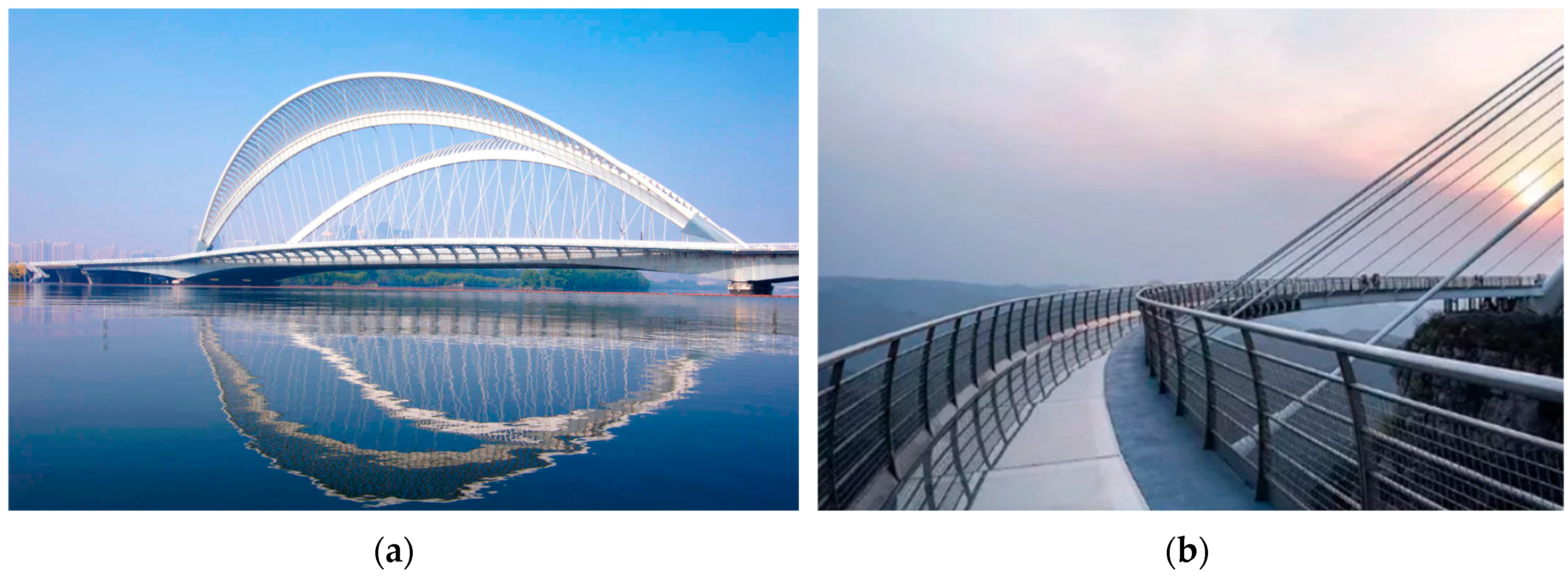
In modern steel bridges and buildings, structural members such as box girders and box arches are typically composed of multiple quadrilateral steel plates (Figure 1). However, bending steel plates into curved shapes is often challenging for curved structural members [1,2,3,4]. Additionally, the bending process exhibits heightened susceptibility to crack initiation in steel plates [5]. Moreover, the metal forming process requires a significant amount of electrical energy. Formed steel consumes approximately 50% more energy compared to flat steel plates [6,7], and the bending process significantly amplifies workload in key carbon-intensive operations, including stiffener welding and flame straightening, which collectively account for 80% of carbon emissions in steel component fabrication [8,9,10,11]. Consequently, the increased utilization of curved plates introduces non-negligible carbon footprint increments that should not be overlooked in sustainable manufacturing assessments. Under current domestic fabrication techniques in China, the comprehensive unit cost of steel structural curved members remains at least 1.3 times that of planar components [12]. To mitigate production expenses, in practical engineering, for elements with small curvature, flat plates are usually substituted during fabrication [13], provided that the following criteria are met: The deviation between the flat plate and the original curved plate remains within permissible tolerances [14,15,16] and the unevenness of the seam between adjacent plates meets the error requirements for welding construction [17,18]. Such substitutions significantly increase fabrication efficiency, reduce project costs, and increase manufacturing sustainability [19].

The engineering community currently addresses such substitution problems through empirical approaches. A critical gap exists in the existing literature regarding systematic discussions of this specific issue. Traditionally, such substitutions rely on trial-and-error estimation by craftsmen [19], which lacks precision and struggles to control construction costs and quality during early project phases.

In recent years, least-squares method (LSM)-based fitting with discrete points [20] has been introduced to solve such problems. In the three-dimensional Cartesian coordinate system, a general plane can be parameterized by coefficients $a$,$b$,$c$ expressed as Equation (1).

$$z=ax+by+c$$

(1)

For a set of points $(x_1,y_1,z_1)$, $(x_2,y_2,z_2)$, …, $(x_n,y_n,z_n)$, a linear equation could be built to find the least-squares plane:

$$\left(\begin{array}{ccc}{x}_1& y_1& 1\\ x_2& y_2& 1\\ ⋮& ⋮& ⋮\\ x_n& y_n& 1\end{array}\right)\left(\begin{array}{c}a\\ b\\ c\end{array}\right)=\left(\begin{array}{c}{z}_1\\ z_2\\ ⋮\\ z_n\end{array}\right)$$

(2)

When $n\ge 3$, the parameters $a$,$b$,$c$ of the least-squares plane for the point set can be obtained by computing the pseudo inverse of the coefficient matrix, as shown in Equation (2). When the original surface patch closely approximates a fitted plane, its boundary can be delineated by projecting it onto the fitted plane, thereby obtaining an approximate planar surface patch, which represents a flat plane in the real world.

While analytical, the least-squares method suffers from limited fitting accuracy. In recent years, some new approaches based on principal component analysis have been proposed [21,22] in a similar field of machine learning, but since they are not designed for geometric fitting, the geometric error is not considered, and this may eliminate some irregular points, which is not suitable for such an engineering problem.

To address these engineering challenges, in this paper, we propose a novel quadrilateral flat plate fitting method that achieves higher precision through the interpolation of fitting errors, offering an enhanced solution for practical applications.

2. Minimum Error Integration Method

2.1. Interpolation Method for Error Evaluation

In order to evaluate fitting error globally, sampling is necessary. To enhance computational efficiency in total error estimation, it is essential to minimize the number of error sampling points. Interpolation is a practical approach to approximate the overall error with a limited set of sample points [23]. This method achieves high accuracy while drastically reducing sampling requirements.

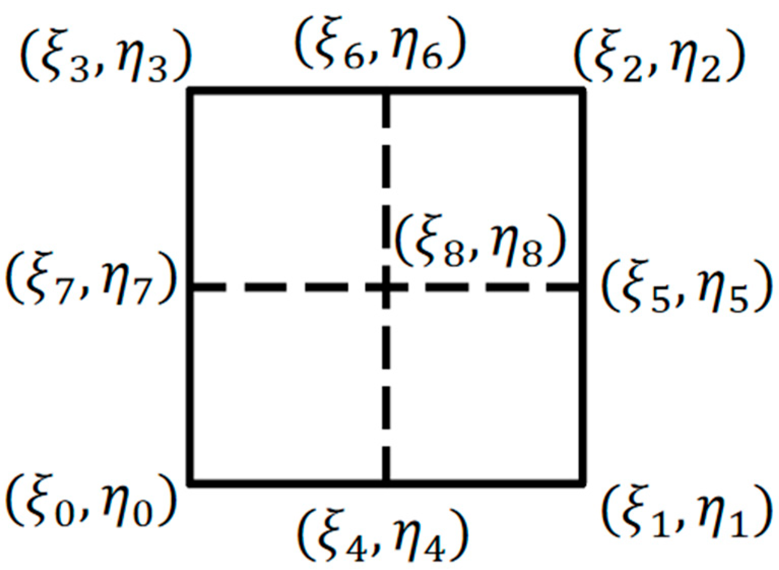
To sufficiently obtain the global error distribution, sampling points should ideally be uniformly distributed across the curved surface. For a bidirectionally uniform $\mathrm{m}\times \mathrm{n}$ grid layout, $(\mathrm{m}+1)\times (\mathrm{n}+1)$ sampling points are required. In typical bridge engineering practice, where the designed curvature variations within steel plates are relatively mild, a $3\times 3$ grid division—sampling at nine key locations (edges, corners, and center of the quadrilateral)—is generally appropriate for quadratic interpolation. For rectangular integration domains, the sampling grid configuration is illustrated in Figure 2.

Lagrange interpolation is a classical polynomial interpolation method [15,16]. The basis functions for full nine-point interpolation are expressed as Equation (3):

$$l_k(\xi )=\prod _{j=0,j\ne k}^2{\displaystyle \frac{\xi -{\xi }_j}{{\xi }_k-{\xi }_j}}$$

(3)

where $k=0,1,2$. and ${\xi }_i$, ${\xi }_j$, ${\xi }_k$ are the ith, jth, and kth nodes in $\xi$ direction.

Likewise, for the $\eta$ direction, the basis functions are expressed as Equation (4):

$$l_k(\eta )=\prod _{j=0,j\ne k}^2{\displaystyle \frac{\eta -{\eta }_j}{{\eta }_k-{\eta }_j}}$$

(4)

where $k=0,1,2$. and $\eta$, ${\eta }_j$, ${\eta }_k$ are the ith, jth, and kth nodes in $\mathsf{\eta }$ direction.

In a two-dimensional rectangular region, the interpolated functions are expressed as Equation (5):

$$N_{3i+j}(\xi ,\eta )=l_i\left(\xi \right)l_j\left(\eta \right)$$

(5)

Then, the error $\mathsf{\delta }$ in any location $(\mathsf{\xi },\mathsf{\eta })$ in the two-dimensional area can be interpolated from sample points as Equation (6):

$$\delta (\xi ,\eta )=\sum _{i=0}^8{N}_i(\xi ,\eta ){\delta }_i$$

(6)

Since the aforementioned Lagrange interpolation applies to rectangular domains, while actual bridge plates in engineering practice often exhibit irregular geometries, isoparametric transformation, which was first used in the finite element method [24,25,26,27], is adopted to compute integrals over non-rectangular regions (Figure 3). In isoparametric transformations, the geometric configuration of arbitrary quadrilateral curved surfaces is similarly represented through interpolation functions that share identical parametric dimensions with the error interpolation scheme. This equivalence in parametric dimensions enables numerical integration of errors over any two-dimensional quadrilateral domain to be computationally evaluated via coordinate transformation to a reference rectangular domain.

The Jacobian matrix of this transformation is defined as follows:

$$J=\left(\begin{array}{cc}{\displaystyle \sum _{i=0}^8}{\displaystyle \frac{\partial N_i(\xi ,\eta )}{\partial \xi }}{x}_i& {\displaystyle \sum _{i=0}^8}{\displaystyle \frac{\partial N_i(\xi ,\eta )}{\partial \xi }}{y}_i\\ {\displaystyle \sum _{i=0}^8}{\displaystyle \frac{\partial N_i(\xi ,\eta )}{\partial \eta }}{x}_i& {\displaystyle \sum _{i=0}^8}{\displaystyle \frac{\partial N_i(\xi ,\eta )}{\partial \eta }}{y}_i\end{array}\right)$$

(7)

This approach converts integrals over free-form regions into standard rectangular domain integrals. The absolute error integral is formulated in Equation (8):

$$\mathsf{\Delta }(\mathit{p})=\iint \delta (\mathit{p},x,y)\mathrm{d}x\mathrm{d}y=\iint \delta (\mathit{p},\xi ,\eta )\mathrm{d}\mathrm{e}\mathrm{t}\left(\mathit{J}\right)\mathrm{d}x\mathrm{d}y$$

(8)

where $\mathsf{\Delta }\left(\mathit{p}\right)$ is the total error in the integration region given a parameter vector $\mathit{p}={(a b c)}^{\mathrm{T}}$, which determines the plane. And $\delta$ is relative to $\mathit{p}$ in this situation, representing the fitting error, which can be taken to be the distance from the point to the plane when the difference between the two is small. And $\mathrm{d}\mathrm{e}\mathrm{t}\left(\mathit{J}\right)$ is the determinant of the Jacobi matrix.

In practice, it is the absolute magnitude of the error rather than the algebraic sum that is of interest. From a numerical computational point of view, squaring makes the local effect of a large absolute value of error magnified and is more conducive to finding the optimal approximation, so the squared error can be used in numerical integration calculations, as shown in Equation (9):

$$\mathsf{\Delta }(\mathit{p})=\iint {\delta }^2(\mathit{p},x,y)\mathrm{d}x\mathrm{d}y=\iint {\delta }^2(\mathit{p},\xi ,\eta )\mathrm{d}\mathrm{e}\mathrm{t}\left(\mathit{J}\right)\mathrm{d}\xi \mathrm{d}\eta$$

(9)

Hence, a standard unconstrained optimization model can be formulated:

$$\underset{\mathit{p}\in {\mathrm{R}}^3}{\min }\mathsf{\Delta }\left(\mathit{p}\right)$$

(10)

2.2. Method for Optimization of the Model Solution

Generally, the convexity of this optimization problem in Equation (10) cannot be guaranteed, and the algorithm’s performance depends critically on the initial guess. If the initial value lies near the optimal solution, convergence to the global optimum can be ensured. In practice, the least-squares solution may serve as the initial guess for subsequent refinement. When the state is sufficiently close to the optimum, the steepest descent method [28]—a gradient-based algorithm using adaptive optimal step sizes—becomes a suitable choice. The algorithm designed for the problem studied in this work is described as follows:

• Initialize ${\mathit{p}}^{<0>}\leftarrow {(a b c)}^{\mathrm{T}}$
• For each time step $t=0,1,2,\dots$, do:
•  Compute gradient $g^{<t>}\leftarrow \nabla ∆\left({\mathit{p}}^{<t>}\right)$
•  Search for optimum step size ${\alpha }^{*}\leftarrow \mathrm{a}\mathrm{r}\mathrm{g}\mathrm{m}\mathrm{i}\mathrm{n}∆({\mathit{p}}^{<t>}-\alpha g^{<t>})$
•  Update: ${\mathit{p}}^{<t+1>}\leftarrow {\mathit{p}}^{<t>}-{\alpha }^{*}{g}^{<t>})$
• Repeat step 2~5 until $\mathit{p}$ converges

In the algorithm described above, the superscript denotes the iteration count for a variable. Since the fitting error is computed via numerical interpolation and integration, the one-dimensional search in Step 4 cannot resolve the analytical minimum through derivative-based methods [29]. To address this, a bisection method is employed for rapid step-size optimization, as detailed below:

• Initialize step size ${{\alpha }_0}^{<0>}\leftarrow 0$, ${{\alpha }_1}^{<0>}\leftarrow 1$
• For each time step $t^{\prime }=0,1,2,\dots$, do:
•  ${{\alpha }_0}^{<t^{\prime }+1>}\leftarrow {{\alpha }_1}^{<t^{\prime }>}$, ${{\alpha }_1}^{<t^{\prime }+1>}\leftarrow {{2\alpha }_1}^{<t^{\prime }>}$
• Until $∆({\mathit{p}}^{<t^{\prime }>}-{{\alpha }_0}^{<t^{\prime }>}{g}^{<t^{\prime }>})<∆({\mathit{p}}^{<t^{\prime }>}-{{\alpha }_1}^{<t^{\prime }>}{g}^{<t^{\prime }>})$, denote this time step as $t^{*}$
• For time step $t^{\prime }=t^{*}+1,{ t}^{*}+2,\dots$, do:
•  If $∆({\mathit{p}}^{<t^{\prime }>}-{{\alpha }_0}^{<0>}{g}^{<t^{\prime }>})<∆({\mathit{p}}^{<t^{\prime }>}-{\displaystyle \frac{1}{2}}({{\alpha }_0}^{<0>}+{{\alpha }_1}^{<0>}\left)g^{<t^{\prime }>}\right)$
•   ${{\alpha }_0}^{<t^{\prime }+1>}\leftarrow {{\alpha }_1}^{<t^{\prime }>}$, ${{\alpha }_1}^{<t^{\prime }+1>}\leftarrow {\displaystyle \frac{1}{2}}({{\alpha }_0}^{<t^{\prime }>}+{{\alpha }_1}^{<t^{\prime }>})$
•  Else
•   ${{\alpha }_0}^{<t^{\prime }+1>}\leftarrow {\displaystyle \frac{1}{2}}({{\alpha }_0}^{<t^{\prime }>}+{{\alpha }_1}^{<t^{\prime }>})$, ${{\alpha }_1}^{<t^{\prime }+1>}\leftarrow {{\alpha }_1}^{<t^{\prime }>}$,
• Repeat step 5~9 until ${\alpha }_0$ converges to ${\alpha }_1$, then take ${{\alpha }^{*}=\alpha }_0$

In the above process, Steps 2 to 4 delineate the interval containing the optimal step size ${\alpha }^{*}$, while Steps 5 to 10 employ the bisection method to search for ${\alpha }^{*}$. The entire procedure, consolidated into an intuitive workflow, is illustrated in Figure 4.

After obtaining the approximate planar surface using the steepest descent method, the boundaries of the original curved plate are projected onto this plane to delineate the boundaries of the approximated flat plate unit. Subsequent verification must confirm compliance with engineering tolerance limits. As demonstrated in the above reference, the convergence of the steepest descent method guarantees a linear convergence rate under appropriate conditions.

3. Results

3.1. Typical Geometry Cases

3.1.1. Shape

Five typical planar shapes, including a square, a rectangle, a parallelogram, a trapezoid, and an arbitrary quadrilateral, were investigated, each under varying curvature conditions, including plane, ruled saddle surfaces, unidirectional/bidirectional convex surfaces, and bidirectional concave–convex surfaces. These fundamental quadrilateral geometries sufficiently represent major engineering scenarios, totaling 25 benchmark cases (

Table 1. Surface shape of the cases.

Case	Square 1 m × 1 m	Rectangle 2 m × 1 m	Parallelogram 1 m × 1 m	Trapezoid 1 m/1.5 m × 1 m	Arbitrary 1 m on Average
Plane κ1 = 0
Ruled surfaces κ1κ2 < 0
Unidirectional convex κ1 > 0 κ2 = 0
Bidirectional convex κ1 > 0 κ2 > 0
Bidirectional concave–convex κ1κ2 < 0

).

3.1.2. Fitting Result

Using a 3 × 3 grid with nine sampling points, the fitting performance of the two methods—the basic least-squares method and the proposed minimum error integration method (MEIM)—was analyzed across surfaces with distinct geometric features, as summarized in

Table 2. Fitting error of the nine-point LSM for different surface shapes.

Case	Square	Rectangle	Parallelogram	Trapezoid	Arbitrary
Plane	0.000	0.000	0.000	0.000	0.000
Ruled saddle	0.028	0.028	0.028	0.026	0.027
Unidirectional convex	0.200	0.200	0.200	0.200	0.200
Bidirectional convex	0.331	0.156	0.156	0.156	0.156
Bidirectional concave–convex	0.226	0.226	0.226	0.225	0.226

.

By taking the least-squares fitting results as initial parameters and applying the proposed minimum error integration method, the results summarized in

Table 3. Fitting error of the proposed MEIM for different surface shapes.

Case	Square	Rectangle	Parallelogram	Trapezoid	Arbitrary
Plane	0.000	0.000	0.000	0.000	0.000
Ruled saddle	0.028	0.028	0.028	0.026	0.027
Unidirectional convex	0.089	0.089	0.089	0.089	0.089
Bidirectional convex	0.081	0.044	0.044	0.044	0.044
Bidirectional concave–convex	0.211	0.211	0.211	0.209	0.210

can be obtained.

The percentage improvement of the proposed minimum error integration method over the least-squares method is tabulated in

Table 4. Improvement of the proposed MEIM fitting.

Case	Square	Rectangle	Parallelogram	Trapezoid	ACQ
Plane	0.0%	0.0%	0.0%	0.0%	0.0%
Ruled saddle	0.0%	0.0%	0.0%	0.0%	0.0%
Unidirectional convex	55.5%	55.5%	55.5%	55.3%	55.5%
Bidirectional convex	75.5%	75.5%	75.5%	75.5%	75.5%
Bidirectional concave–convex	6.9%	6.9%	6.9%	6.9%	6.9%

.

Analysis of the data in Table 4 reveals the following patterns:

• For planar and ruled surface cases, the least-squares method achieves a minimum sum of squared errors, yielding perfectly accurate fits. For ruled saddle surfaces (featuring two orthogonal linear curvature directions), planar approximations exhibit residual errors, though the least-squares method still minimizes squared errors. In both scenarios, the MEIM provides no improvement.
• The MEIM enhances accuracy for other surface types: the improvement for bidirectional concave–concave surfaces is moderate, while the improvement for unidirectional convex and bidirectional convex surfaces is significant.
• The MEIM is planar-shape-independent. The mean squared fitting errors remain largely unaffected by planar geometry variations.

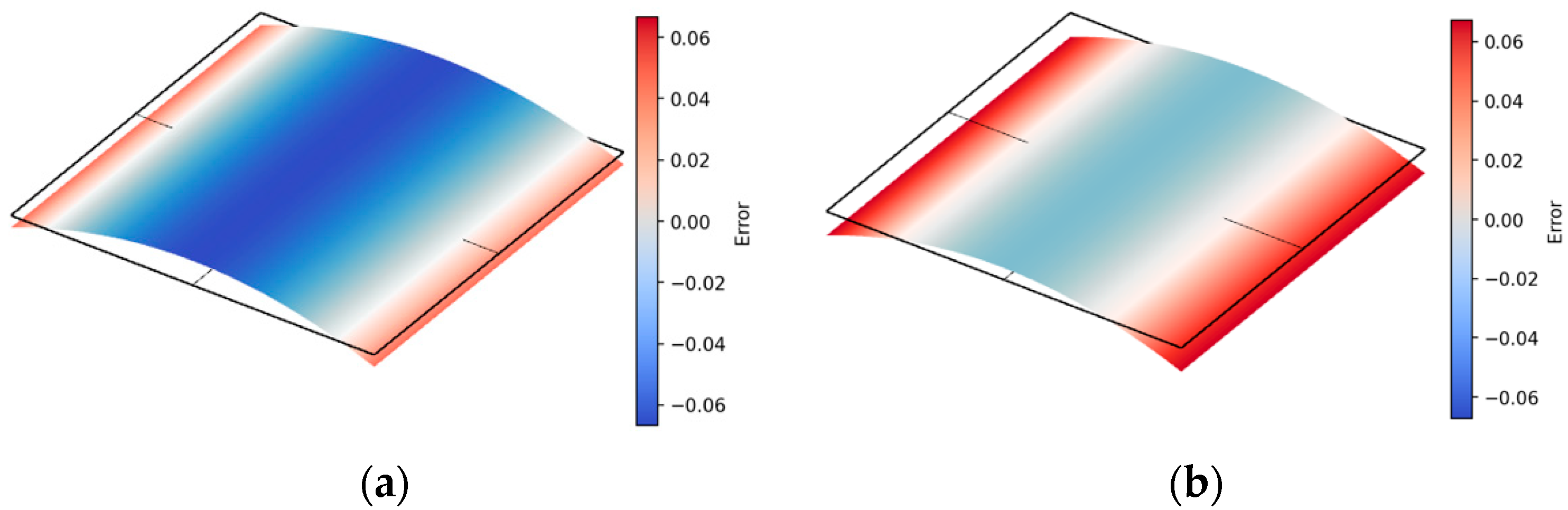
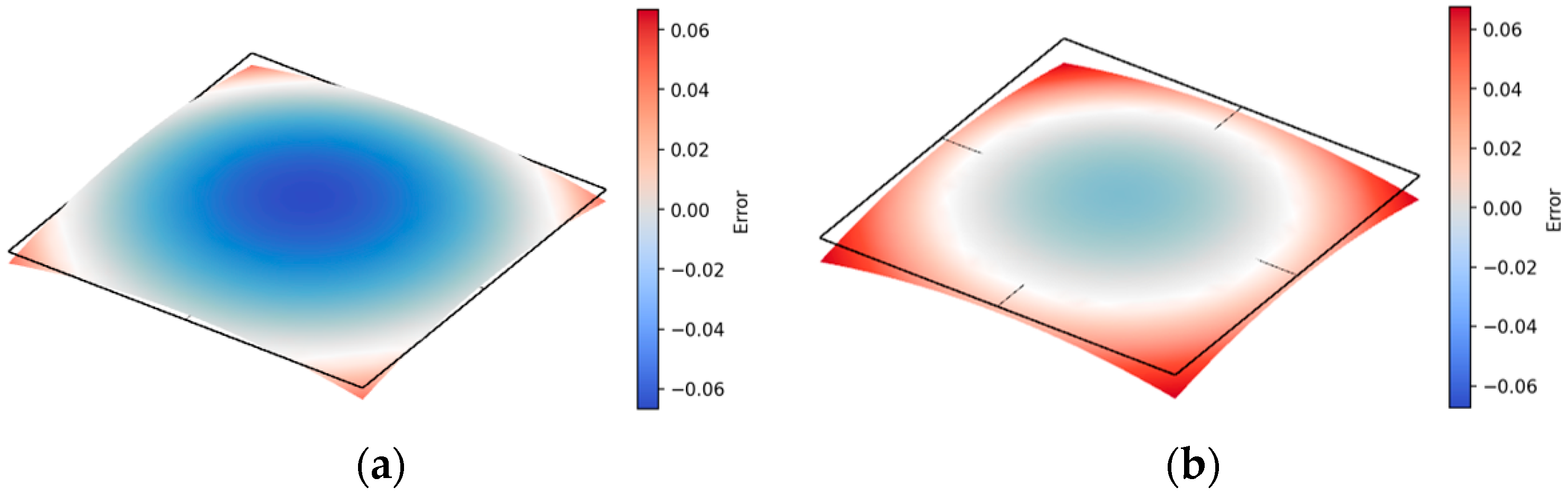
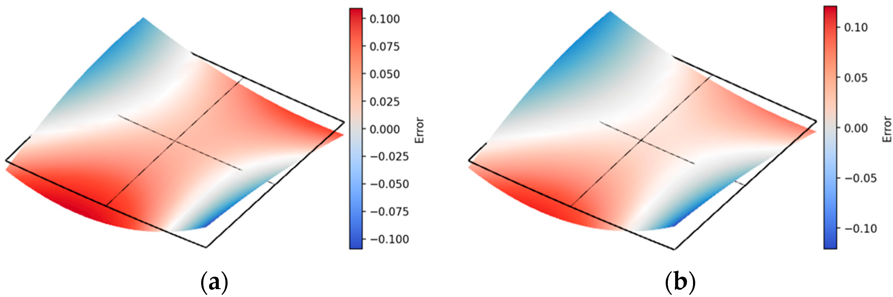
Comparative visualizations of fitting results for distinct surface types—unidirectional convex, bidirectional convex, and bidirectional concave–convex surfaces—are depicted in Figure 5, Figure 6 and Figure 7, with original surfaces rendered in gray and fitted planes rendered in red.

3.2. Practical Engineering Case

3.2.1. Overview

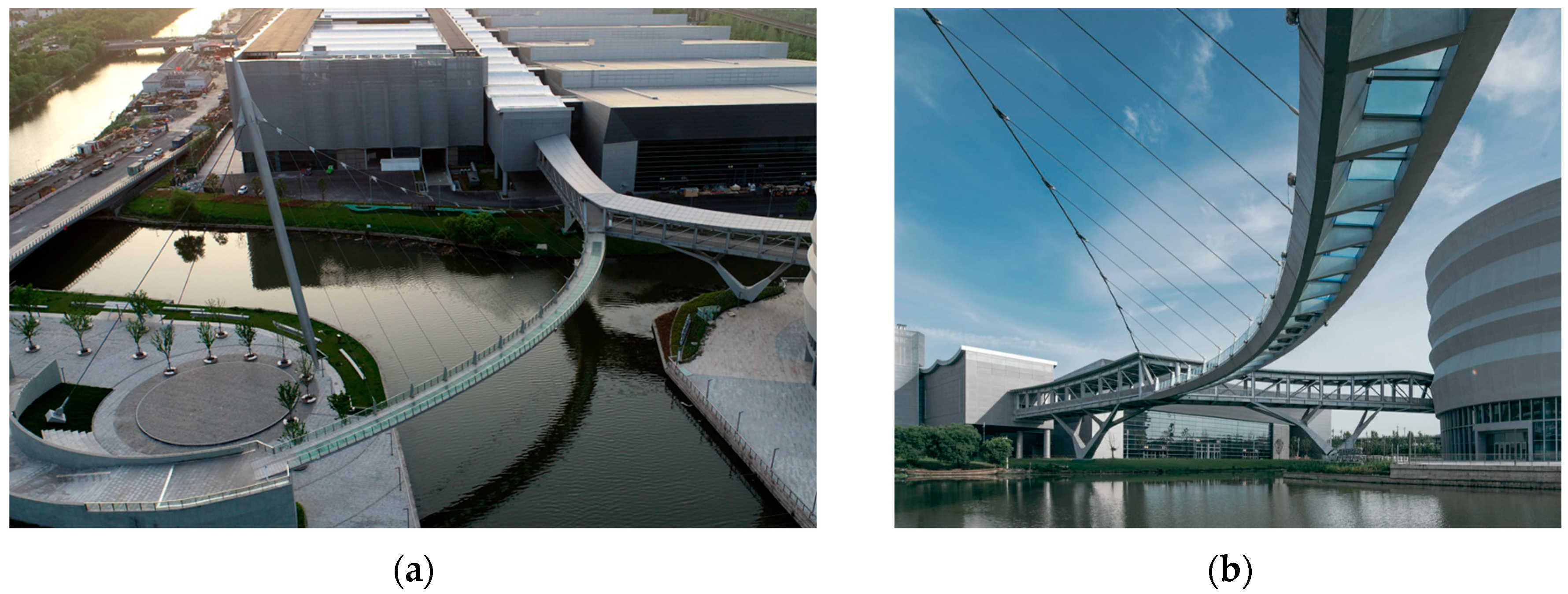
The Pedestrian Bridge at Shaoxing World Convention and Exhibition Center (Shaoxing World) is a curved, lightweight suspension structure spanning 120 m (Figure 8) [30]. The bridge was completed in 2023, and its curved form has significant representativeness in bridge design. Many footbridges around the world have similar curves, including Yuanshan Bridge [31] and Hemei Bridge [32] in China, Footbridge Harbor Grimberg [33] in Europe, and the Liberty Bridge [34] in the United States. Its curved main girder comprises two closed polygonal sections, forming a spatially complex geometry.

The integration of multiple design factors—including a longitudinal gradient along the bridge axis, curved alignment, compound cross-sectional profiles, inclined slope rates, and pre-cambering—imparts biaxial curvature to every steel plate in the structure. However, its slender, cantilevered aesthetic demands exceptionally high fabrication precision.

The structural design strategically balances cost and constructability by optimizing plate geometries to meet economic, aesthetic, and construction quality requirements. The planar and spatial configurations of the main girder are illustrated in Figure 9.

The bridge’s cross-section consists of two longitudinal main girders interconnected by transverse beams. When the main girders follow curved alignments with slope variations, all plates (bottom plates, side plates, etc.) inherently develop biaxial curvature. Given that these plates are externally exposed and require seamless visual continuity, yet curved steel plate fabrication is both technically challenging and cost-prohibitive, meticulous computational verification of each plate’s formed shape is essential to ensure joint compatibility and surface smoothness per design specifications.

The main girder’s steel plates are subdivided into 279 quadrilateral, biaxially curved plate units based on fabrication requirements. In this study, we employ the least-squares method and the minimum error integration method to fit these geometrically complex units into flat plates, thereby streamlining the fabrication of structural components while preserving design integrity.

3.2.2. Feasibility Criteria

In practical engineering, feasibility criteria for plate fitting should align with both fabrication and aesthetic requirements. This typically involves defining maximum error thresholds $\left[{\delta }_{\mathrm{m}}\right]$ and average error thresholds $\left[{\delta }_{\mathrm{a}}\right]$ for decision-making, as shown in Equation (11):

$$\left\{\begin{array}{c}{\delta }_{\mathrm{m}}=\mathrm{m}\mathrm{a}\mathrm{x}\delta (x,y)<\left[{\delta }_{\mathrm{m}}\right]\\ {\delta }_{\mathrm{a}}={\displaystyle \frac{\iint \delta (x,y)\mathrm{d}x\mathrm{d}y}{\iint \mathrm{d}x\mathrm{d}y}}<[{\delta }_{\mathrm{a}}]\end{array}\right.$$

(11)

For this project, the criteria are as follows:

• Welding technical specifications mandate that the maximum deviation between fitted and target plates must not exceed 2 mm;
• Aesthetic considerations require the average deviation across the entire plate surface to remain below 1 mm.

3.2.3. Fitting Result

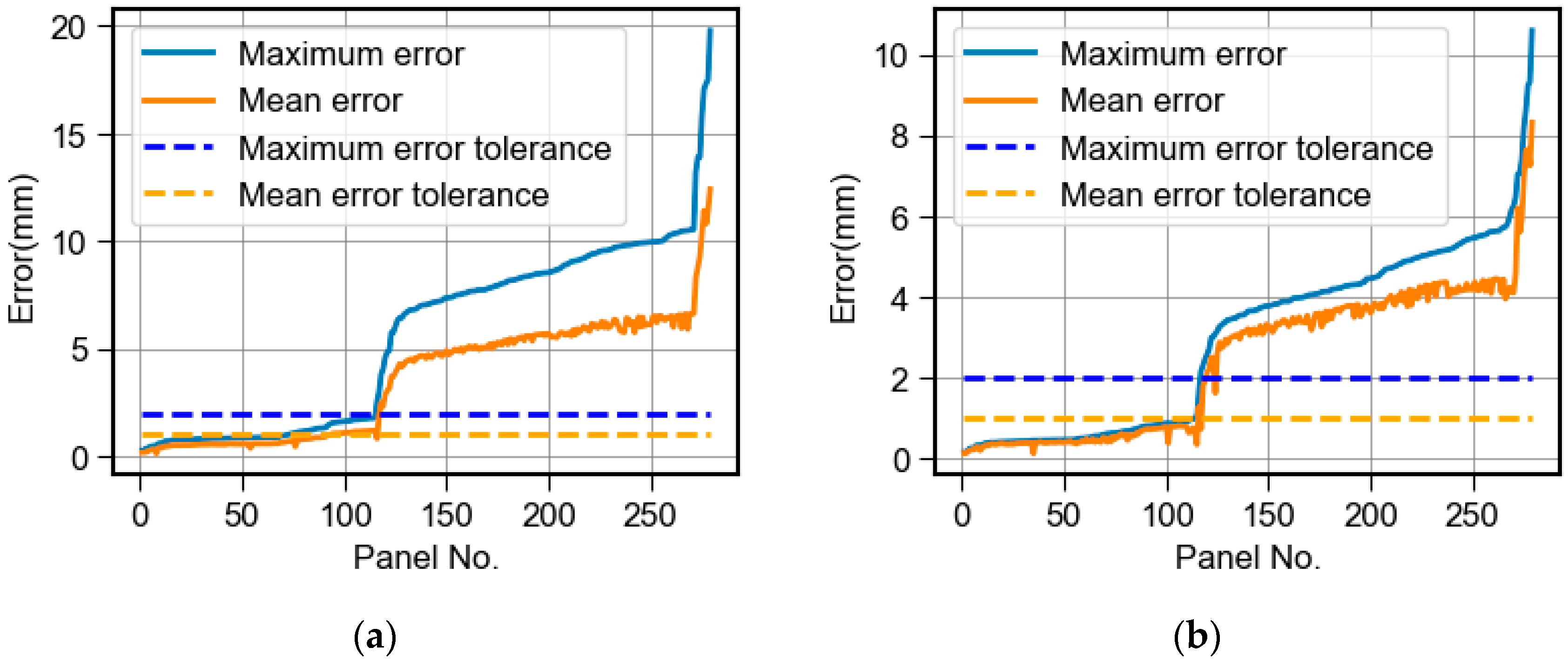
Figure 10 presents the maximum and average fitting errors generated using the least-squares method and the interpolation–integration method for the main girder plates. To enhance visual clarity, the plates are sorted in ascending order based on the max fitting error results, with their data points sequentially connected to form a curve. Correspondingly, the mean fitting error results are plotted, creating the orange curve. Error threshold lines for both maximum and average deviations are annotated in the figure. Compared with the results shown in Figure 10a,b, the results of the MEIM are significantly better than those of the LSM, reducing both the maximum and mean error to about 30–50%, correspondingly.

Another significant observation is that the differential between maximum and average errors in the MEIM results is substantially smaller than in the LSM outcomes, indicating that for each plate segment, the fitting error distribution within the MEIM results demonstrates superior uniformity compared to the LSM. Figure 10 further highlights this contrast: under the specified error thresholds, only about 27% of plates fitted using the least-squares method meet the requirements, whereas the interpolation–integration method achieves compliance for approximately 45% of plates.

Such a result has certain benefits for both the cost and the sustainability of the practical project. For the curved beam section of this project, the steel consumption is approximately 240 tons. Based on the aforementioned optimization results combined with relevant cost data [12] estimates, the LSM demonstrates a cost reduction of approximately RMB 194,400 (equivalent to USD 26,600), while the minimum error integration method (MEIM) achieves savings of RMB 324,000 (USD 44,290). Furthermore, according to carbon emission coefficients derived from the steel structure literature [8,10], the LSM reduces carbon emissions by approximately 5205 kg CO₂, with the MEIM achieving a more substantial reduction of 8676 kg CO₂. This improvement demonstrates that the minimum error integration method enables a greater proportion of curved plates to be replaced with planar approximations without compromising technical or aesthetic standards, thereby significantly enhancing structural cost-effectiveness and manufacturing sustainability.

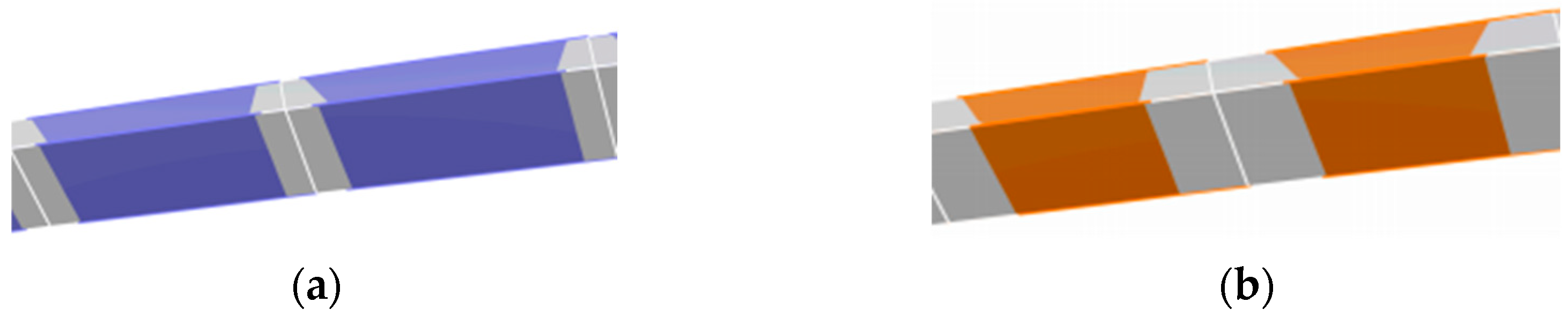
A direct visual comparison of the fitting results is provided in Figure 11. The target biaxially curved plates are rendered in light gray, while the least-squares and interpolation–integration fitted planar plates are shown in blue and orange, respectively. The overlapping color patterns reveal the spatial relationships between the fitted planes and the original curved plates. Notably, the interpolation–integration results exhibit more uniform alignment with the target geometry, with minimized positional deviations compared to the least-squares outcomes.

4. Discussion

In the results shown above, the interpolation–integration approach demonstrably outperforms the least-squares method, particularly for unidirectional and bidirectional convex surfaces. In these cases, the fitted plane aligns more closely with the mid-region of the plate, achieving a globally averaged optimal position. This phenomenon arises from fundamental methodological differences:

The LSM linearly sums errors, yielding exact fits for planar and ruled surfaces where errors inherently follow linear distributions. However, for curved surfaces, its linear weighting disproportionately prioritizes peripheral sampling points, degrading fit quality. But for the MEIM, the Lagrange interpolation adopted has quadratic accuracy, which better accommodates nonlinear error distributions.

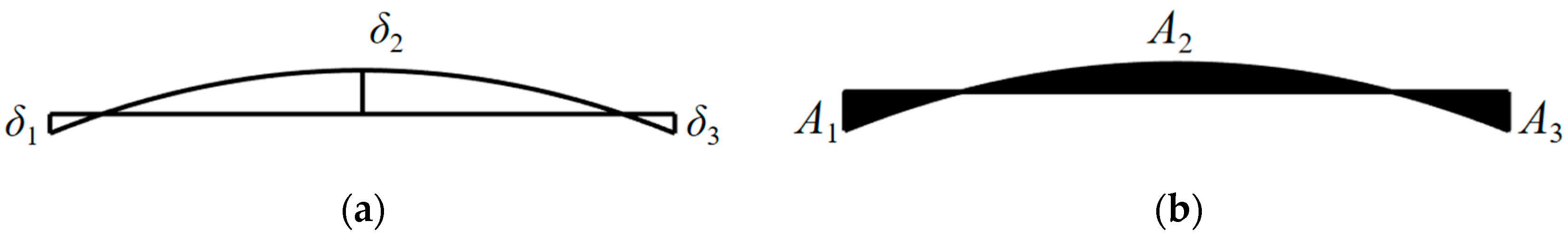
Figure 12 illustrates this contrast: least-squares optimization drives the fitted plane toward error equilibrium at sampling points, minimizing local deviations $\delta$ to the state ${\delta }_2={\delta }_1+{\delta }_3$. The minimum error integration method prioritizes error equilibrium across the integrated area $A$, minimizing cumulative spatial deviations to the state $A_2=A_1+A_3$. Obviously, with limited sampling points, the least-squares method overweights edge regions, whereas interpolation–integration ensures holistic error balancing.

For negative Gaussian surfaces, the two perpendicular curvature directions partially cancel edge-weighting biases, reducing the total error. But for non-negative Gaussian surfaces, the cumulative edge-weighting biases amplify the total error, making the MEIM’s improvements particularly pronounced.

In summary, the principal innovation of the interpolation–integration method lies in quadratic error accommodation through Lagrange interpolation, and the isoparametric transformation’s curvature-agnostic mapping ensures that error variations across geometries primarily stem from numerical computation limits rather than shape differences.

Although the MEIM comprises interpolation and integration, which entails greater computational complexity compared to the LSM, its computation speed remains acceptable when processing limited sample points. The computational analysis in this study was conducted on a workstation equipped with an Intel^® Core™ i7-8700 CPU @ 3.20 GHz (Intel^® Corporation, Santa Clara, CA, USA). The total processing time for individual panel fitting, including pre-processing and post-processing, was recorded as 63 ± 7 ms. Even in large-scale engineering structures requiring the processing of ten thousand panels, the total computation time remains approximately 10 min. This computational efficiency stems from the initial values provided by the least-squares method, which offer high-quality initial guesses that effectively reduce the number of required gradient descent iterations.

The proposed algorithm demonstrates reliable convergence when fitting continuous surfaces, with the adaptive step size calculation preventing oscillations during the optimization process. However, similar to conventional gradient descent approaches, the algorithm guarantees only a local optimum in the vicinity of the least-squares solution rather than the global optimum.

5. Conclusions

In this study, we establish a mathematical model for estimating global fitting errors through interpolation methods and employ the steepest descent algorithm to derive optimal fitting planes. The algorithm’s characteristics are systematically analyzed using both typical geometries and practical engineering cases. The proposed methodology demonstrates the following advantages:

• It achieves high-precision error estimation with minimal sampling points;
• Compared to the LSM, it attains superior quadratic accuracy, and under particular curvature conditions, it achieves over 75% error reduction compared to the LSM;
• While matching the least-squares method’s performance for planar and negative Gaussian curvature surfaces, it significantly outperforms the least-squares method in fitting general convex surfaces;
• Practical cases have verified the effectiveness of the method, increasing the proportion of planarizable plates from 27% to 45%, thus achieving dual benefits in construction cost reduction and carbon emission mitigation for the engineering structure.

It should be acknowledged that the proposed method exhibits certain inherent limitations. The optimization framework employed in this study demonstrates initial condition dependency. While employing least-squares solutions as initial values typically enables rapid convergence to favorable solutions, this approach does not guarantee attainment of the global optimum. Furthermore, when confronted with surfaces exhibiting excessive curvature, planar fitting may fail to maintain geometric errors within acceptable tolerance thresholds. Under such scenarios, the methodology necessitates consideration of alternative canonical surface types, such as cylindrical or conical surfaces, for satisfactory error control.

In summary, the minimum error integration method proposed in this study achieves markedly superior fitting performance for unidirectional or bidirectional convex structural plates compared to the least-squares method. These findings validate the method’s potential to enhance cost-effectiveness and manufacturing sustainability in steel structure projects, suggesting broader applicability in curvature-driven construction scenarios. It is recommended to apply the method proposed in this paper during the steel structure detailing and fabrication phase and integrate it with cost analysis, carbon emission calculation, and automated fabrication systems to further leverage its value in engineering construction.

References

- Weng, C.; White, R. Cold-bending of thick high-strength steel plates. J. Struct. Eng.-ASCE 1990, 116, 40–54. [Google Scholar] [CrossRef]
- Weng, C.; White, R. Residual-stresses in cold-bent thick steel plates. J. Struct. Eng.-ASCE 1990, 116, 24–39. [Google Scholar] [CrossRef]
- Yan, R.; Lin, Y.; Xin, C.; Hu, Y. Research on Residual Stress for Hull Plate in Cold Forming; Zhang, X., Zhang, B., Jiang, L., Xie, M., Eds.; Scientific.Net: Schwyz, Switzerland, 2014; Volume 838–841, pp. 347–354. [Google Scholar]
- Gerbo, E.J.; Thrall, A.P.; Smith, B.J.; Zoli, T.P. Full-Field Measurement of Residual Strains in Cold Bent Steel Plates. J. Constr. Steel Res. 2016, 127, 187–203. [Google Scholar] [CrossRef]
- Jiang, A.; Cheng, Z.; Yu, W. Cause for Cracking of Hot-Rolled Q345 Steel Plate During Roll Bending. Shanghai Met. Chin. 2025, 1–8. [Google Scholar] [CrossRef]
- Norgate, T.E.; Jahanshahi, S.; Rankin, W.J. Assessing the Environmental Impact of Metal Production Processes. J. Clean. Prod. 2007, 15, 838–848. [Google Scholar] [CrossRef]
- Algamal, A.; Ablat, M.A.; Ali, M.; Almotari, A.; Qattawi, A. Manufacturing Energy and Environmental Evaluation of Metallic Sheets Reshaping Based on Theoretical Models and Cradle-to-Gate Assessment. J. Clean. Prod. 2023, 416, 137795. [Google Scholar] [CrossRef]
- Li, Q.; Chen, Z.; Yue, Q.; Feng, P. Research of Carbon Emission in Whole Manufacturing Process of Steel Structure and Carbon Emission Reduction. Build. Struct. Chin. 2023, 53, 8–13. [Google Scholar] [CrossRef]
- Zhang, X.; Chen, H.; Li, R.; Li, Y.; Chen, Z.; Li, J.; Cao, H.; Lin, B.; Zhou, H.; Huang, Z. Research on Carbon Emissions of Production Processes in the Production Stage of Steel Structure Prefabricated Products. Ind. Constr. Chin. 2024, 54, 140–148. [Google Scholar]
- Yang, S.; Zhou, X.; Liu, Z.; Wang, Z.; Liu, X. Research on the Calculation Method of Carbon Emission of Building Steel Structure Manufacturing and Processing Workshop. Build. Sci. Chin. 2023, 39, 19–25. [Google Scholar] [CrossRef]
- Li, Q.; Yue, Q.; Jin, H.; Feng, P. Research Progress on Carbon Emission of Steel Structure Buildings Based on Carbon Peak and Carbon Neutral. Build. Struct. Chin. 2023, 53, 1–7+36. [Google Scholar] [CrossRef]
- China Planning Press. Zhejiang Province Building Construction and Decoration Engineering Budget Quota; China Planning Press: Beijing, China, 2018. (In Chinese) [Google Scholar]
- Hu, W.; Shi, J.; Chen, Y.; Zhu, L.; Zheng, S.; Feng, Q. Fine Modeling of Spatial Three-Dimensional Curved Steel Box Girders Based on BIM Technology. Results Eng. 2025, 25, 103729. [Google Scholar] [CrossRef]
- BS EN 1090-2:2018; Execution of Steel Structures and Aluminium Structures—Part 2: Technical Requirements for Steel Structures. British Standards Institution (BSI): London, UK, 2018.
- GB 20205—2006; Code for Acceptance of Construction Quality of Steel Structure. China Architecture and Building Press: Beijing, China, 2006.
- Australian Steel Institute (AESS). Code of Practice (for Fabricators) Architecturally Exposed Structural Steel (AESS); ASI AESS Document F; Australian Steel Institute (AESS): Sydney, Australia, 2012. [Google Scholar]
- GB 50661—2011; Code for Welding of Steel Structures. China Architecture and Building Press: Beijing, China, 2011.
- ISO 13920:2023; Welding Tolerances for Welded Constructions. ISO: Geneva, Switzerland, 2023.
- Wang, G.; Lin, B. Detailed Design Method of Steel Plate Beam with Straight Instead of Curved. Constr. Des. Proj. Chin. 2023, 102–104. [Google Scholar] [CrossRef]
- Björck, Å. Numerical Methods for Least Squares Problems; Society for Industrial and Applied Mathematics: Philadelphia, PA, USA, 1996. [Google Scholar]
- Feng, C.; Taguchi, Y.; Kamat, V.R. Fast Plane Extraction in Organized Point Clouds Using Agglomerative Hierarchical Clustering. In Proceedings of the 2014 IEEE International Conference on Robotics and Automation (ICRA), Hong Kong, China, 31 May–7 July 2014. [Google Scholar]
- Proenca, P.F.; Gao, Y. Fast Cylinder and Plane Extraction from Depth Cameras for Visual Odometry. In Proceedings of the 2018 IEEE/RSJ International Conference on Intelligent Robots and Systems (IROS), Madrid, Spain, 1–5 October 2018; pp. 6813–6820. [Google Scholar] [CrossRef]
- Greenbaum, A.; Chartier, T.P. Numerical Methods; Princeton University Press: Princeton, NJ, USA, 2012. [Google Scholar]
- Irons, B.M. Engineering Applications of Numerical Integration in Stiffness Methods. AIAA J. 1966, 4, 2035–2037. [Google Scholar] [CrossRef]
- Zienkiewicz, O. The Finite Element Method in Engineering Science; Elsevier: Amsterdam, The Netherlands, 1971. [Google Scholar]
- Zienkiewicz, O.C.; Taylor, R.L.; Taylor, R.L. The Finite Element Method: Basic Formulation and Linear Problems; Elsevier: Amsterdam, The Netherlands, 1989. [Google Scholar]
- Bathe, K.-J. Finite Element Procedures; Prentice Hall: Upper Saddle River, NJ, USA, 1995. [Google Scholar]
- Curry, H.B. The Method of Steepest Descent for Non-Linear Minimization Problems. Q. Appl. Math. 1944, 2, 258–261. [Google Scholar] [CrossRef]
- Strang, G.; Herman, E.P. Calculus; Wellesley-Cambridge Press: Wellesley, MA, USA, 2016. [Google Scholar]
- Huang, Z.; Ding, J.; Xiang, S. Suspension Footbridge Form-Finding with Laplacian Smoothing Algorithm. Int. J. Steel Struct. 2020, 20, 1989–1995. [Google Scholar] [CrossRef]
- SBP Sonne GmbH. Yuanshan Bridge (Xiamen Mountains to Sea Trail). Available online: https://www.sbp.de/en/project/yuanshan-bridge-xiamen-mountains-to-sea-trail/ (accessed on 19 April 2025).
- Yang, Y. Hemei Bridge, Xiamen, China. World Archit. Chin. 2022, 92–95. [Google Scholar] [CrossRef]
- Adriaenssens, S.; Boegle, A. Innovative Structural Typologies. In Innovative Bridge Design Handbook; Elsevier: Amsterdam, The Netherlands, 2022; pp. 215–228. ISBN 978-0-12-823550-8. [Google Scholar]
- Warner, E. Liberty Bridge Celebrates 15th Year. Greenville Journal, 12 September 2019. Available online: https://greenvillejournal.com/community/liberty-bridge-celebrates-15th-year/ (accessed on 19 April 2025).