Article

Modeling the Effects of Vegetation on Air Purification Through Computational Fluid Dynamics in Different Neighborhoods of Beijing

by
Bin Cai
1,
Haomiao Cheng
2,*,
Fanding Xiang
2,
Han Wang
3 and
Tianfang Kang
1
1
Key Laboratory of Beijing on Regional Air Pollution Control, College of Environmental Science and Engineering, Beijing University of Technology, Beijing 100124, China
2
College of Architecture and Urban Planning, Beijing University of Technology, Beijing 100124, China
3
School of Civil Architecture and Environment, Hubei University of Technology, Wuhan 430068, China
*
Author to whom correspondence should be addressed.
Buildings 2025, 15(7), 995; https://doi.org/10.3390/buildings15070995
Submission received: 9 February 2025 / Revised: 3 March 2025 / Accepted: 19 March 2025 / Published: 21 March 2025
(This article belongs to the Section Architectural Design, Urban Science, and Real Estate)

Abstract

Previous research has established that vegetation can significantly improve air quality. However, numerical simulations examining the purification effects of vegetation on air pollutants at the neighborhood scale remain limited, particularly regarding different neighborhood typologies. This study detailed the vegetation, buildings, and pollution emissions within neighborhoods by combining high-resolution imagery with field surveys. Then, a computational fluid dynamics model—validated through field monitoring—was used to design two scenarios to simulate and evaluate the air-purifying effects of vegetation in two typical Beijing neighborhoods. The simulation results were also well validated by the trial-and-error method compared with the computation of vegetation absorption coefficients. Findings indicated that in the Dashilar Traditional Hutong Community, vegetation contributed to reductions of 2.39% in PM2.5 and 3.35% in CO, whereas in the east campus of Beijing University of Technology Pingleyuan, reductions were more substantial, reaching 10.07% for PM2.5 and 8.21% for CO. The results also showed that the size and configuration of green patches directly influence PM2.5 purification efficiency, with consolidated green areas outperforming scattered patches in particle absorption and deposition. Additionally, extensive vegetation near high-rise buildings may not yield the intended purification benefits. These findings provide a robust scientific basis for sustainable urban planning practices aimed at enhancing air quality.

1. Introduction

With rapid urbanization and global warming, city expansion has significantly altered urban surface characteristics. Urban greening, as the only organic infrastructure in urban environments, is essential for fostering a harmonious relationship between humans and nature while enhancing a city’s ecological health [1]. In particular, urban greening plays a key role in improving air quality [2], mitigating the urban heat island effect, reducing air pollution, and stabilizing urban microclimates [3].
Understanding the relationship between vegetation and residential building types is critical to developing sustainable and healthy communities. Liu et al. [4] and Wang et al. [5], respectively, analyzed the impact of green space cluster coverage forms and regional functional types on the surface thermal environment. However, the existing research on this relationship at the neighborhood scale is still insufficient [6]. Particularly, given the limited focus on variation across different neighborhood types [7,8], more studies are needed to comprehensively assess how pollutant distribution interacts with vegetation characteristics and neighborhood building layouts [9]. Moreover, most prior studies have examined the effects of greening on air quality from a two-dimensional perspective, neglecting three-dimensional (3D) analysis [10,11].
Computational fluid dynamics (CFD) models are well-suited for simulating gas dispersion in fluid flow within streets or small neighborhoods from a three-dimensional perspective [12,13]. These models have demonstrated strong capabilities in assessing pollutant dispersion and deposition, including particulate matter [14], NOx [15], VOCs, CO, and O3 [16].
Numerous studies have also focused on the foundational principles of pollutant dispersion in settings such as individual buildings, street canyons, and idealized geometric clusters of buildings [17,18]. However, as the atmospheric environment is inherently open and complex, studies relying on isolated environments or idealized models face inherent limitations.
Plants, due to their unique leaf surface structures and physiological characteristics, can absorb atmospheric particles and contribute to CO absorption [19,20]. However, previous studies examining the relationship between vegetation structure and local air quality often take a reductionist approach, analyzing the effects of microclimates, vegetation, and distribution on regional pollutant concentrations in isolation [21]. The research by Fellini et al. [22] on trees’ air purification effects was limited to the influence of sidewalk trees on pollutant dispersion under ideal conditions. Carlo et al. [23] analyzed the impacts of the regular placement of buildings and trees on pollutant concentrations. Moreover, assessments of vegetation’s air purification effects at the neighborhood scale are typically derived from numerical simulations alone, lacking diverse methods to support these findings [24,25].
Accurately capturing vegetation details within neighborhoods necessitates high-resolution remote sensing imagery [26]. The commonly used 10 m resolution images are significantly larger than the typical size of tree crowns within neighborhoods [27] and, thus, lack the spatial detail needed to represent the actual coverage and fine structure of urban greening [28]. Furthermore, factors such as green ground area and shape complexity impact the surrounding environment and require extraction through ultra-high-resolution imaging data for precise analysis [29].
Using 1 m resolution vegetation distribution data from high-precision imagery, 3D building layout information from on-site surveys, and a combined field-monitoring and CFD simulation approach, this study aimed to comprehensively assess how microclimate, vegetation greening, and building configuration impact neighborhood air quality. In particular, this study analyzed the air purification effects of vegetation from a 3D perspective. The Fluent model was employed to quantify the influence of greening on local air pollutants (PM2.5 and CO—typical pollutants that are both clearly harmful to residents’ health and closely related to the layout of neighborhood buildings and road traffic) across different neighborhood types, with an emphasis on characterizing greening’s purifying effects within typical residential settings. The simulation results were validated through calculations of vegetation absorption coefficients. This study aimed to identify effective relationships between greening and pollutant levels, maximize the purification capacity of greening under limited greening coverage levels, and offer evidence-based guidance on greening design for various neighborhood types.

2. Materials and Methods
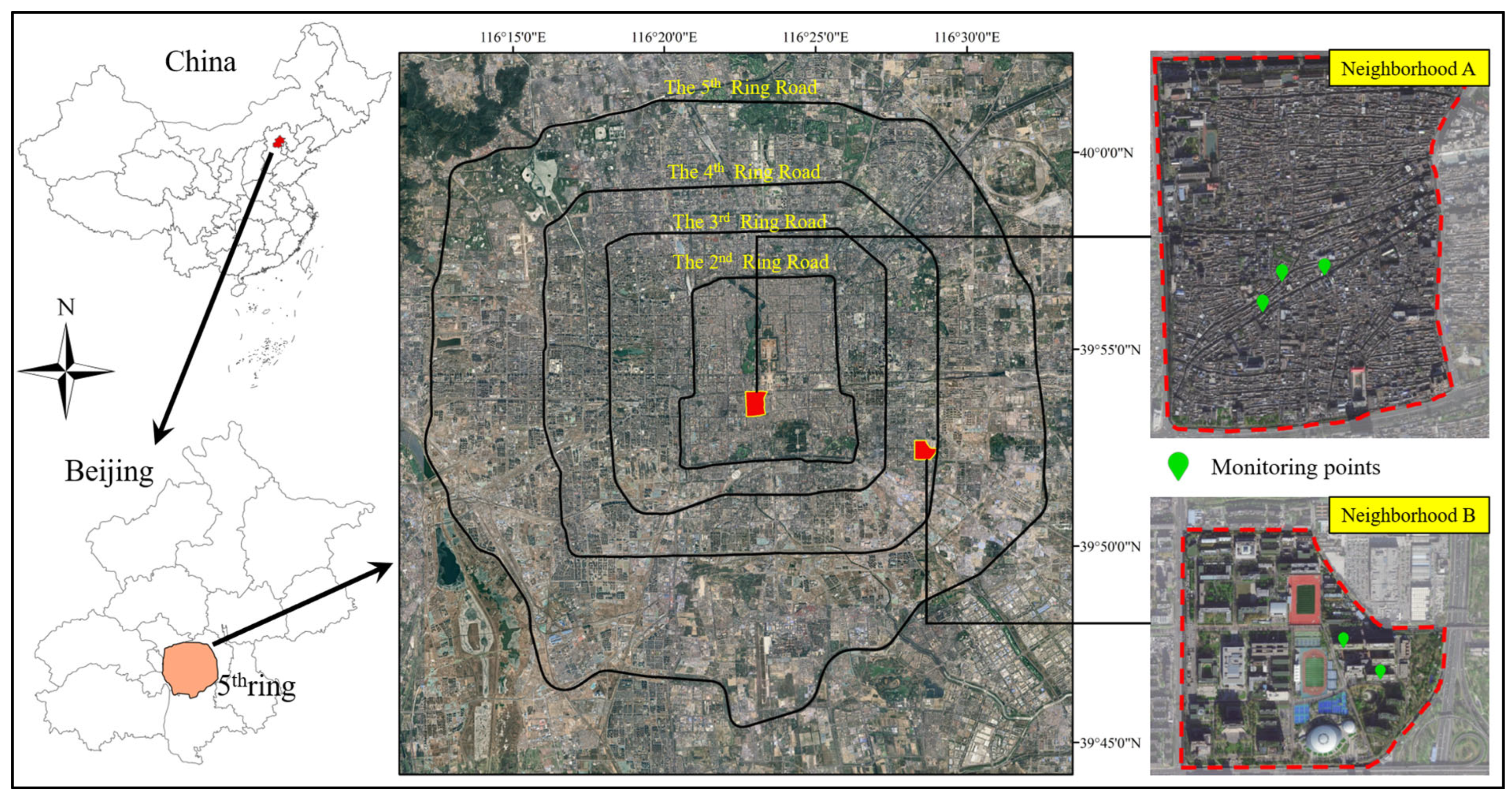
2.1. Study Area

With rapid socioeconomic development, Beijing’s urban green coverage expanded from 22.3% in 1978 to 49.3% in 2021 [30]. The city’s core urbanized area (116.2–116.5° E, 39.8–40.0° N, Figure 1), delineated by the 5th Ring Road, is densely populated, containing 48.9% of the city’s population while covering only 4.1% of its total area. For this study, we selected the Dashilar Traditional Hutong Community (hereafter referred to as Neighborhood A) and the east campus of Beijing University of Technology Pingleyuan (hereafter referred to as Neighborhood B) as research sites. Neighborhood A lies within the 2nd Ring Road, while Neighborhood B is situated at the edge of the 4th Ring Road, each displaying distinct vegetation characteristics.

2.2. Neighborhood Types and Data Collection

Using the 2nd Ring Road as a boundary, we divided Beijing’s core urbanized region into inner and outer areas based on the city’s “figure–ground relationship” and urban growth history. In each area, we selected representative neighborhood types—traditional-style communities in the inner area and cluster-building campus spaces in the outer area—to examine the relationship between their green features and pollution purification effects.
Traditional-style neighborhoods, such as Neighborhood A, occupy 22.09% of the total area and 39.1% of the impermeable surface area (building coverage) in the inner region. In contrast, cluster-building campus spaces, like Neighborhood B, account for 5.56% of the total area and 15.28% of the impermeable surface area in the outer region.
Neighborhood A, one of Beijing’s well-preserved historical and cultural neighborhoods, is characterized by low-rise, beam-framed buildings with a few plate tower structures. It has a dense network of streets and lanes but lacks a cohesive spatial planning scheme. In contrast, Neighborhood B, a cluster-building campus area, is defined by high-rise board tower structures and follows a systematic planning and design approach.
These two are similar in neighboring area size (0.96 and 0.72 km2), population density (301.93 and 291.85 persons/ha), floor area ratio (0.88 and 1.03), and transportation patterns, and both neighborhoods are significantly impacted by traffic pollution due to their proximity to three main and one auxiliary route. However, they differ in building density (63.91% in Neighborhood A vs. 19.62% in Neighborhood B), building height (4.12 m vs. 20.82 m), and green coverage rate (14.33% vs. 48.85%). In the inner area, green coverage in older communities typically falls below 30%, whereas in the outer area, it generally exceeds 30% [31,32].
Data on buildings and streets in traditional-style neighborhoods were obtained from the Beijing Institute of Surveying and Mapping (https://www.bism.cn/ (accessed on 21 September 2023)) and field investigations. Campus space data in the outer area were sourced from 2021 Amap information (via MapOnline, https://www.databox.store/Account/Reg (accessed on 20 September 2023)) and supplemented with building classification details from OpenStreetMap (OSM) (https://download.bbbike.org/osm/ (accessed on 24 September 2023)). Impermeable surface coverage in urban areas was determined using OSM data, with building coverage calculated by excluding natural elements from these surfaces.

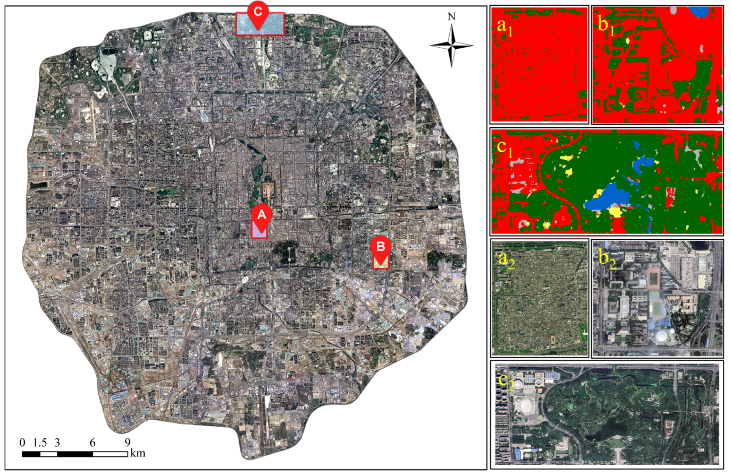
2.3. Mapping of Vegetation Greening

To map the detailed distribution of vegetation greening within the study area, the 10 m resolution greening data from European Space Agency (ESA) WorldCover 2021 [33] was upgraded to a 1 m resolution, following the methodology in [34] and incorporating data from OSM and Google Earth imagery (https://www.google.com/earth/ (accessed on 12 November 2023)). The 1 m resolution greening distribution results provide valuable insights for vegetation selection and identification at the neighborhood scale, serving as a foundation for further exploring the impact of greening distribution on air quality. Detailed vegetation classification information can be found in Supplementary Materials.
Neighborhood A, a historical and cultural district, features a vegetation distribution characterized by fragmented, dispersed, and relatively small patches. To improve the accuracy of vegetation data, this study recalibrated the greening results using ultra-high-resolution 0.3 m imagery from the French Pleiades-NEO satellite, supplemented with local vegetation information obtained through on-site visits. Preprocessing of the remote sensing imagery was carried out using ENVI (v5.2) software to minimize interference and enhance image accuracy. This process included geometric correction, radiometric calibration, atmospheric correction, image stitching, cropping, and other procedures. In Neighborhood B, the vegetation was more concentrated, with larger patches. Recalibration in this area was performed using Google georeferenced images, Amap imagery, campus concept maps, and additional on-site research data for refinement. The accuracy of the vegetation classification results was validated using overall classification accuracy (OA) and the Kappa coefficient. The larger the OA value, the more pixels are correctly classified into their respective categories, while the Kappa coefficient reflects the degree of consistency between the predicted results and the actual classification results. Detailed verification methods can be found in Supplementary Materials.

2.4. Simulation Preprocessing

To ensure the accuracy of the model construction, this study incorporated on-site surveys and satellite image comparisons to calibrate the locations and areas of buildings, vegetation (trees), and public spaces. For Neighborhood A, the underlying data were derived from the 2021 basic survey provided by the Beijing Survey and Design Research Institute. These data underwent dual verification through on-site visits and comparison with remote sensing data to confirm building outlines, footprint areas, heights, and the number of buildings. In Neighborhood B, spatial modeling primarily involved delineating building base outlines through on-site reconnaissance and remote sensing data. Actual building heights and morphological features were cross-referenced with data from BMCHUD [35] and ECBUTY [36]. The model construction process is illustrated in Figure 2.
To investigate the relationship between vegetation distribution and atmospheric pollutants in the neighborhood environment, this study was conducted during the summer season when vegetation exhibited robust growth and had the most significant purification effects on surrounding pollutants. Given the feasibility of on-site monitoring, this research was conducted from 10–24 July 2021. To minimize the influence of drastic meteorological changes on the atmospheric environment, simulated experiments for PM2.5 and CO were performed under clear and breezy weather conditions.
Additionally, the experiment required a comprehensive set of air quality and microclimate data as background information. In this paper, air quality data were collected from national and provincial ambient air quality monitoring stations (https://data.epmap.org/product/nationair (accessed on 18 November 2023)), while microclimate data were derived from surface observations at China Meteorological Administration stations (http://data.cma.cn (accessed on 18 November 2023)). Taking into account factors such as geographical location, wind direction, and surface characteristics, observation data from the Guanyuan and Temple of Heaven national monitoring stations were used as background concentrations for Neighborhood A and Neighborhood B, respectively. The selected days and microclimate characteristics are presented in Supplementary Materials.
To provide the emission source input parameters for the numerical simulation, traffic flow around the research area was investigated during the monitoring period of this study. Since there were no significant point-source emissions around the study area, emissions from motorized traffic on urban roads were identified as the primary source of pollutants. To assess the pollution emission information from roads surrounding the study area, the experiment surveyed the length and width of both the surrounding and internal roads. Using the on-site counting method, a traffic survey was conducted during the period from 10:00 to 11:00 a.m. to capture traffic flow data around Neighborhoods A and B. Additionally, traffic flow data from within the campus road network of Neighborhood B were also collected. The road traffic flow and emission intensity data are detailed in Supplementary Materials.

2.5. CFD Numerical Simulation

This study used ANSYS-Fluent 2020R1 for CFD solving to simulate the comprehensive spatiotemporal dispersion of pollutants within the research area [37], focusing on the greening purification effects of two representative urban neighborhoods on the diffusion and absorption of gaseous pollutants. To evaluate the purification effect of neighborhood green coverage on environmental pollutants, assuming relatively stable atmospheric conditions, this study employed scenario analysis by conducting numerical simulation experiments for two parallel scenarios: BIO and NOBIO. The BIO scenario incorporated a 3D model that included both buildings and vegetation cover, while the NOBIO scenario used a 3D model of buildings alone for comparison.
The simulation conditions were based on the guidelines provided by Franke et al. [38] and Goddard et al. [39]. The Reynolds-averaged Navier–Stokes RNG K-ε model, as recommended by Antoniou et al. [40] and Issakhov and Omarova [41], was selected to model air pollution dispersion in complex urban geometries. The finite volume method was employed to discretize the governing equations. The pressure-coupled SIMPLE algorithm (second-order upwind scheme) was used for the solution process. Euler equations were applied for numerical concentration calculations of pollutants. To prevent divergence during the iteration process, under-relaxation techniques were implemented for pressure, density, momentum, turbulent kinetic energy, and the turbulence dissipation rate. Convergence residuals for continuity, momentum, turbulent kinetic energy, and dissipation rate equations were set to 10−4. Additional boundary condition information can be found in Supplementary Materials.
Based on the two-dimensional mapping of the research area and actual building heights, this study conducted detailed modeling within the designated red-line boundaries using AutoCAD (v2020). The model incorporated the calibrated existing building structures, vegetation data models, and roads that allow vehicular traffic emissions of air pollutants. While retaining geometric features, the model simplified non-smooth appearances. The computational domain’s horizontal and vertical spacing was maintained at a distance of 5 H (where H is the height of the tallest building in the model) from the outermost points of the modeling area, as recommended by Franke et al. [42]. The final dimensions of the computational domain are illustrated in Figure 2.
To reduce computational costs, a non-structured grid system, dominated by hexahedral elements, was employed to partition the computational domain. Local refinement was applied around buildings, with an adjacent grid growth rate of less than 1.2. Additionally, prism grids were generated near the walls to accommodate wall function conditions. Considering the hardware capabilities of the computer, three grid schemes (coarse, medium, and fine) were established to simulate the same environment according to best practices to ensure the numerical results were independent of the grid count. After performing grid independence tests, the minimum and maximum grid sizes were set to 0.5 m and 10 m, respectively. The final number of grid nodes for Neighborhood A and Neighborhood B were determined to be 1.3 × 10⁸ and 4.2 × 10⁶, respectively, with grid quality exceeding 0.3 in both cases.
According to the results of the vegetation classification, the greening within the 5th Ring Road area of the city was primarily composed of deciduous tree species, while other vegetation types such as shrubs and grasslands were predominantly found outside the 5th Ring Road. Consequently, all vegetation within the study area was modeled as arbor trees. Based on the greening survey information, the CFD model assumed an average tree height of 5 m and a homogeneous tree structure. To account for the impact of trees on the surrounding airflow, which reduces wind speed and increases airflow disturbance, this study employed a porous medium model for the tree canopy. This was achieved by adding a momentum source (sink) term to the standard fluid flow equations. The source term consists of two components: a viscous loss term (Darcy) and an inertial loss term. The porosity was set at 0.7, the inertial resistance at 0.18, and the viscous resistance at 1.67 [43]. Further details on conventional parameterization are provided in Supplementary Materials.
To enhance the sample data for parameters and optimize statistical processing, the research neighborhoods were rasterized into 20 units, each with a base size of 250 m × 250 m, as shown in Figure 3. A cross-section at a height of 1.5 m above the ground (typical breathing height for pedestrians) was chosen to illustrate the spatial distribution of PM2.5 and CO pollutants. During the simulation process, area-weighted average pollutant concentration values were extracted from the 20 units for comparative analysis after the pollutant dispersion reached convergence.

2.6. Validation of CFD Results

Field monitoring was conducted to validate the reasonableness of the simulated results for pollutant concentrations. This study employed the XL68 environmental monitoring equipment (Xinli Technology Co., Ltd., Shenzhen, China) to monitor the microclimate and pollutant concentrations within the neighborhoods. A real-time air environment monitoring system was established to enable 24 h automated data collection. Detailed information about the sensor instrumentation is provided in Supplementary Materials.
The operation of the environmental monitoring equipment adhered to technical specifications [44], with sensors positioned approximately 3 m above the ground. The monitoring points were chosen in areas free from obstructing high-rise buildings, trees, or other obstacles, ensuring unobstructed air circulation. Additionally, monitoring points were placed in the central areas of the study area to minimize the influence of nearby road traffic pollution. Finally, 3 monitoring points for Neighborhood A and 2 for Neighborhood B were chosen, with their locations shown in Figure 1.
Field monitoring data from 39 stations, including national and provincial ambient air quality automatic monitoring stations, as well as neighborhood monitoring stations, were used. The spatial distribution of pollutant concentrations was interpolated using the Empirical Bayes Kriging method. The resulting spatial distributions of PM2.5 and CO concentrations during the monitoring period were mapped in ArcGIS to predict pollutant levels in the study neighborhoods. In the simulated neighborhood, concentration data from 20 equidistant points were extracted for comparison and validation with the simulation results. The simulation results were considered valid if the magnitude of PM2.5 and CO volume fractions matched the observed concentrations in the monitoring data [45].
To assess the validity of the simulation, SPSS (v25.0) software was used, and a t-test was applied to determine whether there was a significant difference between the observed and simulated values. The results, shown in Table 1 with a significance value (sig.) greater than 0.05, indicated no significant difference between the observed and simulated data, confirming that the simulation accurately predicts the actual environmental conditions [46].

2.7. Vegetation Absorption Coefficient

Additionally, the greening purification effects in the BIO scenario were validated using the vegetation absorption coefficient. Vegetation absorbs various gaseous pollutants and aerosols through leaf stomata, with varying absorption capacities for each pollutant. In this study, the total amount of pollutants absorbed by vegetation in the neighborhoods during the study period was calculated based on the actual greening area and the vegetation absorption coefficient for CO and PM2.5.
Considering that the simulation experiment in this study was conducted during clear summer weather, the average dust retention index of PM2.5 per unit leaf area for tree species in the study area was determined to be 0.09 g/m2 based on the summer dust retention data on various northern dominant tree species (see Supplementary Materials). Referring to the research by Jin et al. [47] and Chen et al. [48], the absorption capacity of vegetation for PM2.5 within a specific range was calculated using Equation (1).
Q = L A I v · C · S
where Q (kg·hm−2·h−1) is the PM2.5 absorption capacity, LAIv is the leaf area index per unit area, C is the dust retention index, and S (hm2) is the total green coverage area within the study area. The LAI for the study area within the 5th Ring Road of Beijing was obtained by collecting and reclassifying the 2021 HiQ-LAI product [49]. The results were then extracted and weighted averaged to obtain a unified LAIv of 4.0.
For CO, the absorption coefficient was derived by converting the CO2 absorption coefficient based on the relative molecular mass ratio. The results for the CO2 absorption coefficients of different vegetation cover types were referenced from Aly et al. [19], and the conversion formula is as follows. The vegetation absorption coefficient for CO was calculated as 82.68 g·ha−1·h−1.
M R C O M R C O 2 = M C O M C O 2
where MRCO (g·ha−1·h−1) and MRCO2 (g·ha−1·h−1) are the CO absorption coefficient and CO2 absorption coefficient, respectively. MCO (g) and MCO2 (g) are the relative molecular weights of CO and CO2, respectively.

3. Results

3.1. Vegetation Greening Distribution

The distribution of vegetation greening within the neighborhoods is illustrated in Figure 4. The validation results showed that, within the 5th Ring Road in Beijing in 2021, the OA of the greening classification was 80.7%. Among the three validation neighborhoods, the OA ranked as follows: Olympic Forest Park (82.3%) > Neighborhood B (79.2%) > Neighborhood A (74.5%). The Kappa coefficient was 0.73, indicating a good consistency between the classified results and the actual land cover types.

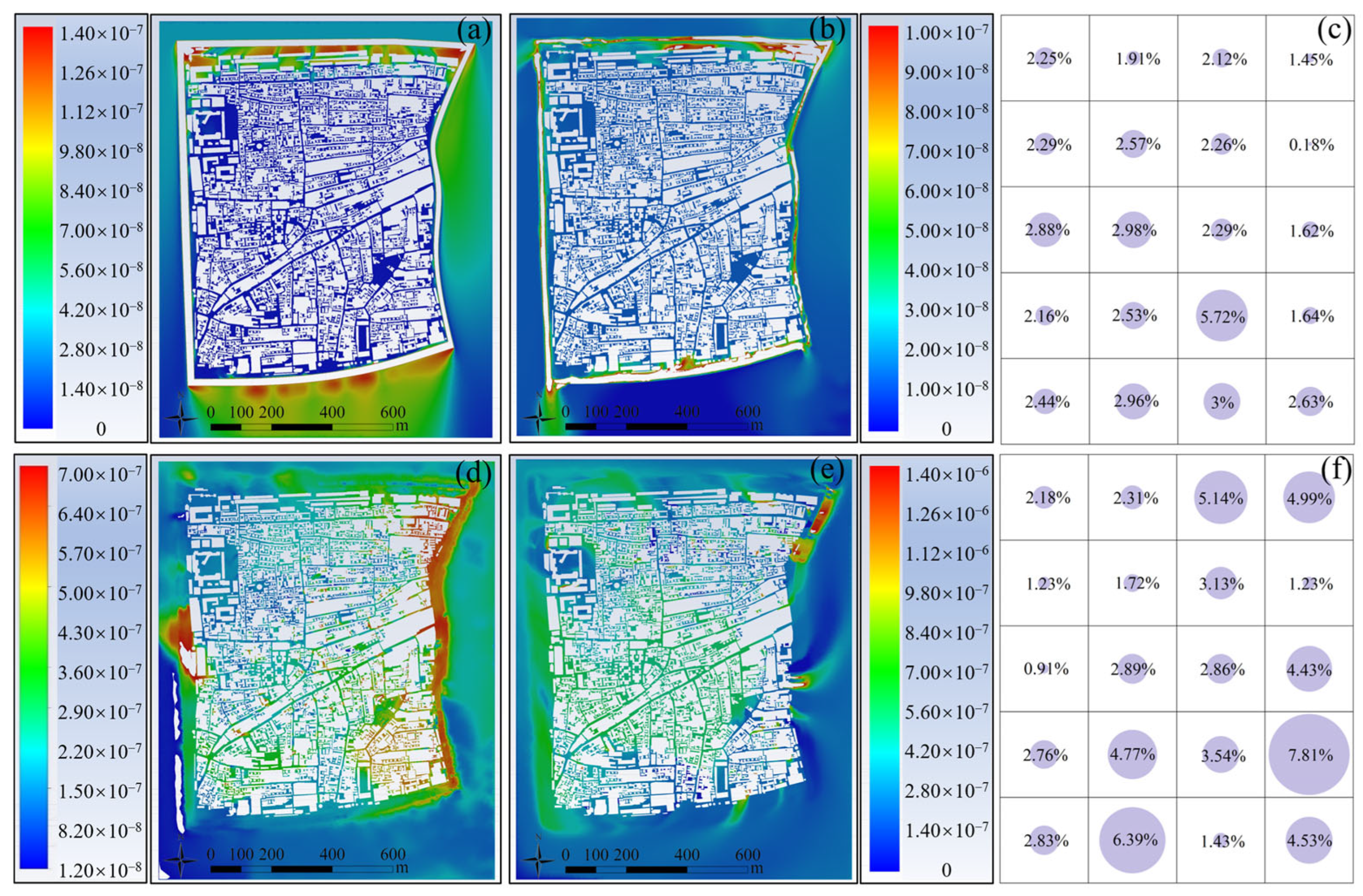
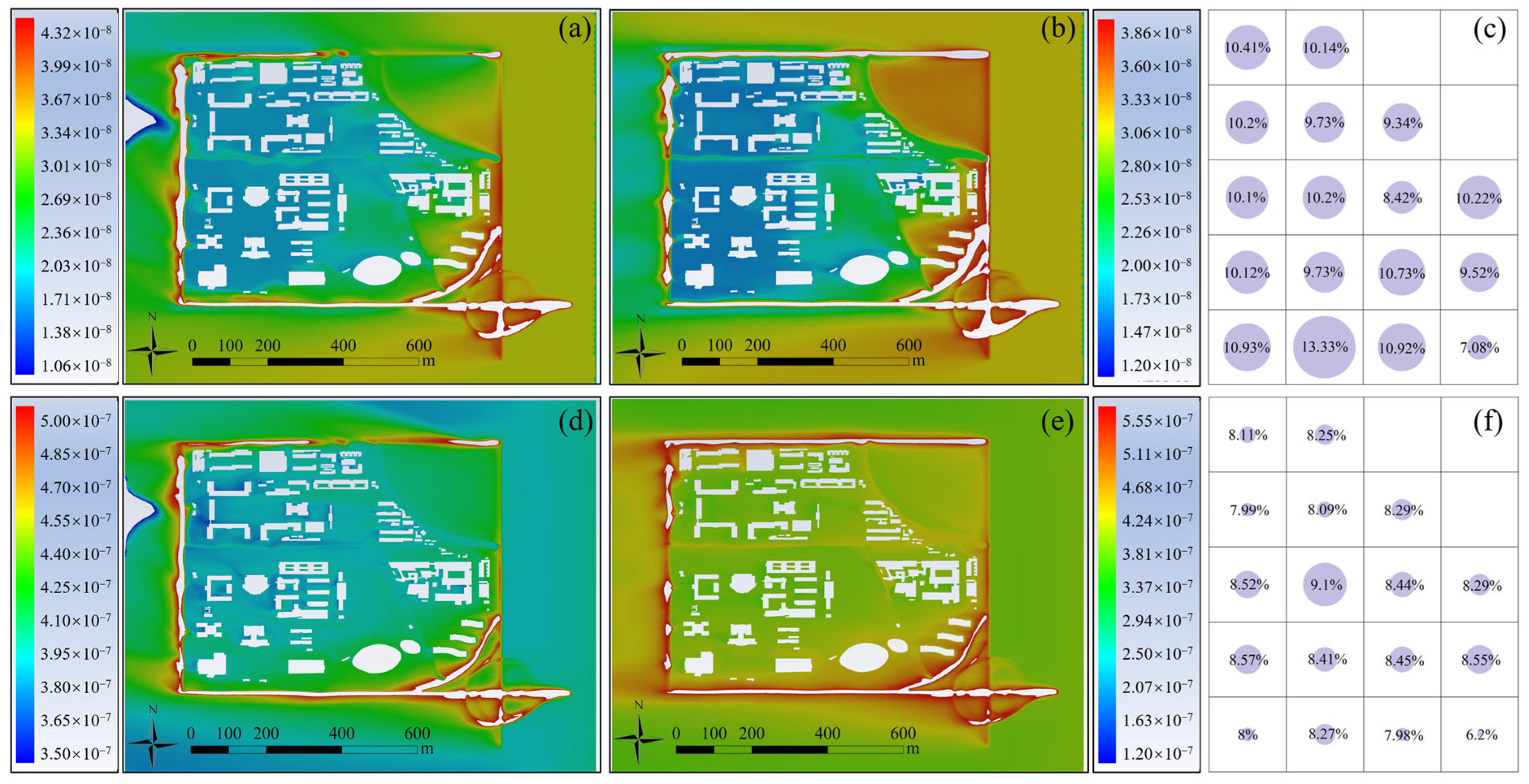
3.2. Pollutant Concentration Difference in Neighborhoods

By comparing the simulated air pollutant concentrations in Neighborhoods A and B under the BIO/NOBIO scenarios, insights into the impact of greening on regional PM2.5 and CO concentrations within urban neighborhoods can be gained, as well as an understanding of how the greening purification effects vary across different neighborhood types.
Comparative analysis was conducted using the simulated pollutant concentration values of the 20 research units in Neighborhood A, with the mean simulation values representing pollutant concentration variations across the entire neighborhood. Comparing the simulation results between the BIO and NOBIO scenarios, it was evident that the greening in Neighborhood A led to a 2.39% decrease in the PM2.5 concentration, closely matching the 2.63% decrease in the simulated values at three monitoring points. The CO concentration decreased by 3.35%, aligning well with the 3.67% reduction in the simulated values at these points. The pollutant dispersion effect is illustrated in Figure 5.
In the overall neighborhood environment, pollutants exhibited a diffusion pattern along the road network, particularly in the downwind direction of the dominant wind. A comparative analysis of simulated values at the 20 points revealed that the reduction in PM2.5 concentration was more spatially varied than CO. Specifically, the concentration reduction in PM2.5 at points 1–8 in the northern part of the study area was significantly lower than at points 9–20 in the southern part, with the northern points showing an average reduction of 1.88% and the southern points showing a 2.74% reduction, which was 45.74% higher.
Considering that research units 3, 4, and 8 are outside Neighborhood B, the pollutant concentration values of the remaining 17 research units were selected for comparative analysis. The mean simulation values were used to represent pollutant concentration variations across the entire neighborhood. Comparing the simulation results between the BIO and NOBIO scenarios, it is evident that the greening in Neighborhood B led to a 10.07% decrease in the PM2.5 concentration, which closely matched the 8.69% decrease in the simulated values at two monitoring points. The CO concentration decreased by 8.21%, aligning well with the 8.25% reduction in the simulated values at these points. The pollutant dispersion effect is illustrated in Figure 6.

3.3. Vegetation Greening Absorption

In Neighborhood A, the greening area measures 13.76 hectares, allowing for the purification of 495.4 g of PM2.5 and 1137.77 g of CO from the air. In Neighborhood B, with a greening area of 31.26 hectares, the vegetation can purify 1125.42 g of PM2.5 and 2584.7 g of CO.
Based on the BIO scenario, emission levels from road traffic were incrementally increased using a trial-and-error approach, with PM2.5 and CO source intensities in the Fluent model raised to match pollution dispersion levels observed in the NOBIO scenario while keeping other conditions constant. This adjustment reflects the actual impact of vegetation on PM2.5 and CO absorption and deposition in the environment. Figure 7 illustrates the relationship between increased source emissions and environmental pollutant concentrations. The results show that when PM2.5 source emissions increased by 370 g and CO emissions by 950 g, the simulated PM2.5 and CO concentrations in Neighborhood A were comparable to those in the NOBIO scenario. Similarly, in Neighborhood B, the simulated PM2.5 and CO concentrations closely matched those of the NOBIO scenario with an increase of 860 g in PM2.5 and 2250 g in CO source emissions.

4. Discussion

4.1. Greening Purification Effects in Neighborhoods

Overall, the NOBIO scenario exhibited higher PM2.5 and CO concentrations compared to the BIO scenario, indicating that open green spaces contribute to improved environmental quality in Neighborhoods A and B. Greening, unlike artificial surfaces, can more effectively remove atmospheric pollutants and eliminate particles through deposition [2,50]. Compared with the simulation results for Neighborhood A, Neighborhood B experienced a significantly greater reduction in pollutant concentrations, likely due to its noticeably higher green coverage. This finding suggests that expanding green areas within a certain range enhances environmental benefits. Selmi et al. [51] similarly noted that larger greenspace areas, such as forests and parks, in urban regions lead to greater reductions in particulate matter levels. When green coverage in the neighborhood environment reached nearly 50%, ambient pollutant concentrations for PM2.5 and CO were effectively reduced by 8% to 10%.
In Neighborhoods A and B, vegetation greening exhibited varying effects on PM2.5 and CO purification. In Neighborhood A, the reduction in CO concentration was greater than that for PM2.5 in the BIO scenario, whereas the opposite trend was observed in Neighborhood B. The greening in Neighborhood B was arranged in larger, more concentrated patches with fewer, more cohesive areas, leading to good connectivity. In contrast, Neighborhood A’s green spaces were highly fragmented, with many smaller and scattered patches. For particle deposition and absorption, the clustered greening distribution in Neighborhood B appeared to favor its scale effect, preventing fine particles adhered to vegetation surfaces from being re-suspended into the air by airflow or released after entrapment, which could otherwise elevate local PM2.5 concentrations. Similar findings have been reported in previous studies [52,53]. Additionally, clustered tree plantings can create a multi-layered greening structure [54,55], effectively reducing the atmospheric particulate circulation. For neighborhoods facing high particulate matter pollution and fixed green areas, avoiding a fragmented green patch distribution and encouraging the clustering of greening can improve pollutant removal and reduce wind resistance effects while fulfilling residents’ needs.
In the northern units of Neighborhood A, the green cover rate is significantly higher than in other units; however, the overall vegetation purification effect remains limited. Considering the arrangement of high-rise buildings along the road edges in units 1 and 2, it can be assumed that planting substantial greening near high-rise buildings may not be optimal, as the purification effect is constrained. Firstly, the close proximity and narrow spacing of these high-rise structures obstruct sunlight, which impedes surrounding plants from reaching their full growth potential and results in reduced foliage density. Since foliage is essential for pollutant deposition and absorption, particularly for pollutants like PM2.5 and CO [56,57], sparse foliage lowers the efficacy of greening in purifying air. Secondly, the significant height contrast between high-rise buildings and nearby low-rise structures generates complex eddy currents that create high wind speeds in these areas [58]. These wind patterns disrupt stable pollutant deposition, as the air pollutant exchange rate decreases, hindering consistent purification and absorption by greening [59]. Consequently, the conditions around densely packed high-rises are less conducive to effective pollutant removal through vegetation.
During the simulation period, the prevailing wind in Neighborhood B was observed to blow from the east, leading to a significant impact from pollutant emissions originating from eastern roads. In the eastern part of the neighborhood, large concentrations of greening blocked and retained PM2.5 and CO emissions, effectively preventing these pollutants from permeating further into the neighborhood environment. As shown in Figure 6, PM2.5 and CO concentrations are relatively high on the eastern edge of the neighborhood but decrease markedly after passing through the eastern greening, with PM2.5 levels showing a more substantial reduction than CO. This difference is attributed to the nature of PM2.5, which, as solid particles, is denser than air and more susceptible to gravitational settling. Consequently, the spread of PM2.5 pollutants from the east becomes more stagnant and precipitates out more readily. In contrast, CO, with a density almost identical to air, is less affected by gravity, allowing for stronger downwind diffusion. For future neighborhood planning and design, it is advisable to plant vegetation in areas exposed to prevailing winds, particularly in zones where pollutant emissions are prevalent. Strategically positioned greening can act as a natural barrier between residential spaces and external pollution sources, effectively reducing the entry of pollutants into the neighborhood.

4.2. Comparison and Verification of the Vegetation Absorption Coefficient

Compared to the simulation results, both methods displayed relatively good consistency, with PM2.5 and CO reductions based on the vegetation absorption coefficient appearing slightly higher than simulated values. This difference is anticipated, as the absorption coefficient reflects a macroscopic statistical estimate of vegetation’s pollutant absorption capacity, whereas actual absorption depends on factors such as vegetation characteristics, meteorological conditions, and ambient pollutant concentrations [60]. This leads to some discrepancies with simulation results, which account for building layouts, local microclimate, gravity effects, greening structure, and other details.
One reason for the difference is that the absorption coefficient method overlooks vegetation’s influence on surrounding wind fields, focusing solely on pollutant absorption. Wind is critical in gas pollutant transport; however, vegetation can also impede airflow, reducing pollutant dispersion and dissipation in the environment. As a result, PM2.5 disperses less effectively. Additionally, high-rise building configurations can create eddy zones on the windward side under low-wind conditions, obstructing fresh air inflow and facilitating PM2.5 accumulation in surrounding areas.
Furthermore, there is also potential for overestimation despite using a synthesized dust retention index derived from pre-human findings. This coefficient assumes saturation on the leaf surface, although, in practice, absorption and deposition rarely reach this level. PM2.5 absorption on leaf surfaces increases with higher PM2.5 concentrations [60]. However, PM2.5 levels in the study area were relatively low during the monitoring period, meaning that the dust retention index may be somewhat inflated.

4.3. Research Limitations and Future Directions

This study has several limitations despite addressing some research gaps in previous studies. First, while plants absorb atmospheric pollutants and influence air exchange and ventilation [61], they also emit volatile organic compounds that can impact atmospheric composition [62]. Some of these compounds act as precursors in the formation of fine particles, and under certain environmental conditions, their interactions with atmospheric compounds may locally increase PM2.5 concentrations. Second, this study treated a limited number of shrubs and herbaceous plants as trees and set a uniform tree height and porosity for all trees due to the difficulty of gathering thorough information on tree height and branch structure and the time expense. Finally, in order to study the relationship between vegetation greening and pollutant distribution under stable conditions, this study assumed that the input rate of road traffic emissions is constant to achieve steady-state simulation. However, in reality, various emission rates and intensities will occur during vehicle operation due to idling, congestion, and other factors.
Future studies could extend the geographical area, including dynamic variables (e.g., climate change), refine models with advanced techniques, or integrate broader environmental factors while considering the potential negative effects of vegetation on pollutants for a more comprehensive study [63]. This sets directions for further research.

5. Conclusions

The relationship between urban populations and neighborhood atmospheric conditions is closely connected, with open green spaces in neighborhoods contributing significantly to improved air quality. This study combined neighborhood greening information from high-resolution imagery and field surveys with spatial building data, using the Fluent model to assess the impact of greening distribution and planting levels on PM2.5 and CO pollutants within inner-ring, traditional-style neighborhoods and outer-ring, campus-style neighborhoods. This study’s findings offer architects, urban planners, and policymakers a scientific foundation for urban design strategies aimed at enhancing urban air quality. The main conclusions are as follows:
(1)
Increasing the green coverage rate can be conducive to the purification of PM2.5 and CO when the rate is below 50%. According to this study’s results, a neighborhood green coverage of nearly 50% can effectively reduce ambient pollutant concentrations by 8% to 10%.
(2)
The size of green patches directly influences their purification effect on PM2.5 particles. In neighborhoods with severe PM2.5 pollution, more thought should be given to arranging fewer, clustered green patches rather than fragmented ones, which can more effectively remove PM2.5 and other particulates from the environment.
(3)
Large-scale greening has little effect on air purification in areas with dense high-rise buildings. In community design, greening should be arranged more in open spaces with less height variation between buildings. For high-rise structures, vertical greening might be a viable option.
(4)
Future neighborhood planning and design should prioritize vegetation in areas aligned with prevailing wind patterns, which can significantly reduce PM2.5 and CO pollutant influx.

Supplementary Materials

The following supporting information can be downloaded at: https://www.mdpi.com/article/10.3390/buildings15070995/s1, References [48,64,65,66,67,68,69,70,71,72,73,74,75,76].

Author Contributions

Conceptualization, B.C. and H.C.; methodology, B.C.; formal analysis, B.C.; investigation, F.X.; software, F.X.; data curation, H.W. and T.K.; writing—original draft preparation, B.C.; writing—review and editing, H.C.; resources, H.W.; visualization, F.X.; supervision, H.C. and T.K.; funding acquisition, H.C. All authors have read and agreed to the published version of the manuscript.

Funding

This work was supported by the National Natural Science Foundation of China (No. 52170174).

Data Availability Statement

The data presented in this study are available on request from the corresponding author.

Conflicts of Interest

The authors declare no conflicts of interest.

References

  1. Nielsen, A.B.; van den Bosch, M.; Maruthaveeran, S.; van den Bosch, C.K. Species richness in urban parks and its drivers: A review of empirical evidence. Urban Ecosyst. 2014, 17, 305–327. [Google Scholar] [CrossRef]
  2. Janhäll, S. Review on urban vegetation and particle air pollution—Deposition and dispersion. Atmos. Environ. 2015, 105, 130–137. [Google Scholar]
  3. Matos, P.; Vieira, J.; Rocha, B.; Branquinho, C.; Pinho, P. Modeling the provision of air-quality regulation ecosystem service provided by urban green spaces using lichens as ecological indicators. Sci. Total Environ. 2019, 665, 521–530. [Google Scholar] [CrossRef] [PubMed]
  4. Liu, W.; Zhao, H.; Sun, S.; Xu, X.; Huang, T.; Zhu, J. Green space cooling effect and contribution to mitigate heat island effect of surrounding communities in Beijing metropolitan area. Front. Public Health 2022, 10, 870403. [Google Scholar]
  5. Wang, Y.; Yang, S. Identification of surface thermal environment differentiation and driving factors in urban functional zones based on multisource data: A case study of Lanzhou, China. Front. Environ. Sci. 2024, 12, 1466542. [Google Scholar]
  6. Guyot, M.; Araldi, A.; Fusco, G.; Thomas, I. The urban form of Brussels from the street perspective: The role of vegetation in the definition of the urban fabric. Landsc. Urban Plan. 2021, 205, 103947. [Google Scholar]
  7. Buccolieri, R.; Jeanjean, A.P.; Gatto, E.; Leigh, R.J. The impact of trees on street ventilation, NOx and PM2.5 concentrations across heights in Marylebone Rd street canyon, central London. Sustain. Cities Soc. 2018, 41, 227–241. [Google Scholar]
  8. Borna, M.; Turci, G.; Marchetti, M.; Schiano-Phan, R. Evaluating the influence of urban blocks on air pollution concentration levels: The case study of Golden Lane Estate in London. Sustainability 2024, 16, 696. [Google Scholar] [CrossRef]
  9. Zhang, Z.; Li, Y.; Li, M.; Meng, H.; Zhang, T.; Peng, Z.; Zhang, W. Improving atmospheric particulate matter removal of residential green space based on landscape patterns and plant functional types. Air Qual. Atmos. Health 2023, 16, 401–413. [Google Scholar]
  10. Xu, J.; Liu, M.; Chen, H.; Luo, M. Spatially heterogeneous influence of street greenery on street-level PM2.5 pollution using mobile monitoring from a three-dimensional perspective. Urban Clim. 2023, 48, 101414. [Google Scholar]
  11. Bahr, S. The relationship between urban greenery, mixed land use and life satisfaction: An examination using remote sensing data and deep learning. Landsc. Urban Plan. 2024, 251, 105174. [Google Scholar] [CrossRef]
  12. Bachir, N.; Bounoua, L.; Aiche, M.; Maliki, M.; Nigro, J.; El Ghazouani, L. The simulation of the impact of the spatial distribution of vegetation on the urban microclimate: A case study in Mostaganem. Urban Clim. 2021, 39, 100976. [Google Scholar]
  13. Mohammadi, M.; Tien, P.W.; Calautit, J.K.S. Influence of wind buffers on the aero-thermal performance of skygardens. Fluids 2020, 5, 160. [Google Scholar] [CrossRef]
  14. Karttunen, S.; Kurppa, M.; Auvinen, M.; Hellsten, A.; Järvi, L. Large-eddy simulation of the optimal street-tree layout for pedestrian-level aerosol particle concentrations—A case study from a city-boulevard. Atmos. Environ. X 2020, 6, 100073. [Google Scholar]
  15. Komalasari, D.; Shi, Z.; Harrison, R.M. Optimisation of a numerical model to simulate the dispersion and chemical transformations within the oxides of nitrogen/ozone system as traffic pollution enters an urban greenspace. Earth Syst. Environ. 2021, 5, 927–937. [Google Scholar]
  16. Tiwari, A.; Kumar, P. Integrated dispersion-deposition modelling for air pollutant reduction via green infrastructure at an urban scale. Sci. Total Environ. 2020, 723, 138078. [Google Scholar] [PubMed]
  17. Lin, C.; Ooka, R.; Kikumoto, H.; Sato, T.; Arai, M. CFD simulations on high-buoyancy gas dispersion in the wake of an isolated cubic building using steady RANS model and LES. Build. Environ. 2021, 188, 107478. [Google Scholar] [CrossRef]
  18. Lin, X.; Fu, Y.; Peng, D.Z.; Liu, C.-H.; Chu, M.; Chen, Z.; Yang, F.; Tse, T.K.T.; Li, C.Y.; Feng, X. CFD- and BPNN-based investigation and prediction of airpollutant dispersion in urban environment. Sustain. Cities Soc. 2024, 100, 105029. [Google Scholar]
  19. Aly, S.H.; Zakaria, R.; Kondorura, C.F. The capability of green open space in absorbing carbon monoxide and carbon dioxide emissions in Balai Kota Makassar. IOP Conf. Ser. Earth Environ. Sci. 2020, 419, 012169. [Google Scholar]
  20. Leonard, R.J.; McArthur, C.; Hochuli, D.F. Particulate matter deposition on roadside plants and the importance of leaf trait combinations. Urban For. Urban Green. 2016, 20, 249–253. [Google Scholar]
  21. Liu, J.; Zheng, B. A simulation study on the influence of street tree configuration on fine particulate matter (PM2.5) concentration in street canyons. Forests 2023, 14, 1550. [Google Scholar] [CrossRef]
  22. Fellini, S.; Marro, M.; Del Ponte, A.V.; Barulli, M.; Soulhac, L.; Ridolfi, L.; Salizzoni, P. High resolution wind-tunnel investigation about the effect of street trees on pollutant concentration and street canyon ventilation. Build. Environ. 2022, 226, 109763. [Google Scholar] [CrossRef]
  23. Carlo, O.S.; Fellini, S.; Palusci, O.; Marro, M.; Salizzoni, P.; Buccolieri, R. Influence of obstacles on urban canyon ventilation and air pollutant concentration: An experimental assessment. Build. Environ. 2024, 250, 111143. [Google Scholar] [CrossRef]
  24. Wang, Y.; Flageul, C.; Maison, A.; Carissimo, B.; Sartelet, K. Impact of trees on gas concentrations and condensables in a 2-D street canyon using CFD coupled to chemistry modeling. Environ. Pollut. 2023, 323, 121210. [Google Scholar] [CrossRef] [PubMed]
  25. Ysebaert, T.; Koch, K.; Samson, R.; Denys, S. Green walls for mitigating urban particulate matter pollution—A review. Urban For. Urban Green. 2021, 59, 127014. [Google Scholar] [CrossRef]
  26. Qian, Y.; Zhou, W.; Li, W.; Han, L. Understanding the dynamic of greenspace in the urbanized area of Beijing based on high resolution satellite images. Urban For. Urban Green. 2015, 14, 39–47. [Google Scholar] [CrossRef]
  27. Guo, J.; Liu, Z.; Zhu, X. Assessing the macro-scale patterns of urban tree canopy cover in Brazil using high-resolution remote sensing images. Sustain. Cities Soc. 2024, 100, 105003. [Google Scholar] [CrossRef]
  28. Ludwig, C.; Hecht, R.; Lautenbach, S.; Schorcht, M.; Zipf, A. Mapping public urban green spaces based on OpenStreetMap and Sentinel-2 imagery using belief functions. ISPRS Int. J. Geo-Inf. 2021, 10, 251. [Google Scholar] [CrossRef]
  29. Yan, L.; Jia, W.; Zhao, S. The cooling effect of urban green spaces in metacities: A case study of Beijing, China’s capital. Remote Sens. 2021, 13, 4601. [Google Scholar] [CrossRef]
  30. BMBS (Beijing Municipal Bureau of Statistics). Beijing Statistical Yearbook 2022; China Statistics Press: Beijing, China, 2022. [Google Scholar]
  31. GB 50137-2011; Code for Classification of Urban Land Use and Planning Standards of Development Land. MHUDPRC (Ministry of Housing and Urban-Rural Development of the People’s Republic of China): Beijing, China; China Architecture & Building Press: Beijing, China, 2011.
  32. CJJ/T 85-2017; Standard for Classification of Urban Green Space. MHUDPRC (Ministry of Housing and Urban-Rural Development of the People’s Republic of China): Beijing, China; China Architecture & Building Press: Beijing, China, 2017.
  33. Zanaga, D.; Van De Kerchove, R.; Daems, D.; De Keersmaecker, W.; Brockmann, C.; Kirches, G.; Wevers, J.; Cartus, O.; Santoro, M.; Fritz, S. ESA WorldCover 10 m 2021 v200. Zenodo 2022. [Google Scholar] [CrossRef]
  34. Li, Z.; Zhang, H.; Lu, F.; Xue, R.; Yang, G.; Zhang, L. Breaking the resolution barrier: A low-to-high network for large-scale high-resolution land-cover mapping using low-resolution labels. ISPRS. J. Photogramm. 2022, 192, 244–267. [Google Scholar]
  35. BMCHUD (Beijing Municipal Commission of Housing and Urban-Rural Development). Beijing Construction Yearbook 2021; Beijing University of Technology Press: Beijing, China, 2021. [Google Scholar]
  36. ECBUTY (Editorial Committee of Beijing University of Technology Yearbook). Beijing University of Technology Yearbook 2021; Beijing University of Technology Press: Beijing, China, 2021. [Google Scholar]
  37. ANSYS Inc. FLUENT Training Material—ANSYS 2020 Version R1, Lecture Transient Flow Modeling, Introduction to ANSYS Fluent; ANSYS Inc.: Canonsburg, PA, USA, 2020. [Google Scholar]
  38. Franke, J.; Hellsten, A.; Schlunzen, K.H.; Carissimo, B. The COST 732 best practice guideline for CFD simulation of flows in the urban environment: A summary. Int. J. Environ. Pollut. 2011, 44, 419–427. [Google Scholar] [CrossRef]
  39. Goddard, K.A.; Craig, K.J.; Schoombie, J.; le Roux, P.C. Investigation of ecologically relevant wind patterns on Marion Island using computational fluid dynamics and measured data. Ecol. Model. 2022, 464, 109827. [Google Scholar] [CrossRef]
  40. Antoniou, N.; Montazeri, H.; Wigo, H.; Neophytou, M.K.A.; Blocken, B.; Sandberg, M. CFD and wind-tunnel analysis of outdoor ventilation in a real compact heterogeneous urban area: Evaluation using “air delay”. Build. Environ. 2017, 126, 355–372. [Google Scholar] [CrossRef]
  41. Issakhov, A.; Omarova, P. Numerical simulation of pollutant dispersion in the residential areas with continuous grass barriers. Int. J. Environ. Sci. Technol. 2020, 17, 525–540. [Google Scholar] [CrossRef]
  42. Franke, J.; Sturm, M.; Kalmbach, C. Validation of OpenFOAM 1.6.x with the German VDI guideline for obstacle resolving micro-scale models. J. Wind. Eng. Ind. Aerodyn. 2012, 104, 350–359. [Google Scholar]
  43. Zhang, P.; Cheng, H.; Jiang, Z.; Xiang, F. How sensitive morphological parameters influence on the PM2.5 diffusion: An empirical study of two neighborhoods in central Beijing. Atmosphere 2022, 13, 921. [Google Scholar] [CrossRef]
  44. HJ 664-2013; Technical Regulation for Selection of Ambient Air Quality Monitoring Stations. MEEPRC (Ministry of Ecology and Environment of the People’s Republic of China): Beijing, China; China Environmental Science Press: Beijing, China, 2013.
  45. Zheng, L.; Lu, W.; Wu, L.; Zhou, Q. A review of integration between BIM and CFD for building outdoor environment simulation. Build. Environ. 2023, 228, 109862. [Google Scholar]
  46. Xu, X.; Gao, Z.; Zhang, M. A review of simplified numerical approaches for fast urban airflow simulation. Build. Environ. 2023, 234, 110200. [Google Scholar]
  47. Jin, E.J.; Yoon, J.H.; Bae, E.J.; Jeong, B.R.; Yong, S.H.; Choi, M.S. Particulate matter removal ability of ten evergreen trees planted in Korea urban greening. Forests 2021, 12, 438. [Google Scholar] [CrossRef]
  48. Chen, B.; Lu, S.W.; Zhao, Y.G.; Li, S.N.; Yang, X.B.; Wang, B.; Zhang, H.J. Pollution remediation by urban forests: PM2.5 reduction in Beijing, China. Pol. J. Environ. Stud. 2016, 25, 1873–1881. [Google Scholar]
  49. Yan, K.; Wang, J.; Weiss, M.; Myneni, R.B. A High-Quality Reprocessed MODIS Leaf Area Index Dataset (HiQ-LAI; v1). Zenodo 2023. [Google Scholar] [CrossRef]
  50. Buccolieri, R.; Santiago, J.-L.; Rivas, E.; Sanchez, B. Review on urban tree modelling in CFD simulations: Aerodynamic, deposition and thermal effects. Urban For. Urban Green. 2018, 31, 212–220. [Google Scholar]
  51. Selmi, W.; Weber, C.; Rivière, E.; Blond, N.; Mehdi, L.; Nowak, D. Air pollution removal by trees in public green spaces in Strasbourg city, France. Urban For. Urban Green. 2016, 17, 192–201. [Google Scholar]
  52. Pallozzi, E.; Guidolotti, G.; Mattioni, M.; Calfapietra, C. Particulate matter concentrations and fluxes within an urban park in Naples. Environ. Pollut. 2020, 266, 115134. [Google Scholar]
  53. Yin, Z.; Zhang, Y.; Zhang, R.; Chen, G.; Cong, Y.; Ma, K. Structure of an urban green space indirectly affects the distribution of airborne particulate matter: A study based on structural equation modelling. Urban For. Urban Green. 2022, 72, 127581. [Google Scholar]
  54. Chen, X.; Wu, J.; Yang, W.; Wang, Z.; Chen, S.; Hu, X.; Lu, K.; Fan, Z.; Lin, M.; Chen, P. Measuring and modeling the effects of green barriers on the spatial distribution of fine particulate matter at roadside. Urban Clim. 2023, 52, 101727. [Google Scholar]
  55. Wu, J.; Long, J.; Liu, H.; Sun, G.; Li, J.; Xu, L.; Xu, C. Biogenic volatile organic compounds from 14 landscape woody species: Tree species selection in the construction of urban greenspace with forest healthcare effects. J. Environ. Manag. 2021, 300, 113761. [Google Scholar] [CrossRef]
  56. Duan, X.; Gu, H.; Lam, S.S.; Sonne, C.; Lu, W.; Li, H.; Chen, X.; Peng, W. Recent progress on phytoremediation of urban air pollution. Chemosphere 2024, 349, 140821. [Google Scholar] [CrossRef]
  57. Li, H.; Zhu, X.; Kong, W.; Zheng, M.; Guo, X.; Wang, T. Physiological response of urban greening shrubs to atmospheric particulate matter pollution: An integral view of ecosystem service and plant function. Environ. Exp. Bot. 2023, 213, 105439. [Google Scholar]
  58. Kuo, C.; Wang, R.; Lin, Y.; Lai, C. Urban design with the wind: Pedestrian-level wind field in the street canyons downstream of parallel high-rise buildings. Energies 2020, 13, 2827. [Google Scholar] [CrossRef]
  59. Wen, Y.; Huang, Z.; Tang, Y.; Li, D.; Zhang, Y.; Zhao, F. Air exchange rate and pollutant dispersion inside compact urban street canyons with combined wind and thermal driven natural ventilations: Effects of non-uniform building heights and unstable thermal stratifications. Sci. Total Environ. 2022, 851, 158053. [Google Scholar] [PubMed]
  60. Lind’en, J.; Gustafsson, M.; Uddling, J.; Watne, A.; Pleijel, H. Air pollution removal through deposition on urban vegetation: The importance of vegetation characteristics. Urban For. Urban Green. 2023, 81, 127843. [Google Scholar] [CrossRef]
  61. Jeanjean, A.P.R.; Buccolieri, R.; Eddy, J.; Monks, P.S.; Leigh, R.J. Air quality affected by trees in real street canyons: The case of Marylebone neighbourhood in central London. Urban For. Urban Green. 2017, 22, 41–53. [Google Scholar]
  62. Hsu, K.-W.; Chao, J.-C. Economic valuation of green infrastructure investments in urban renewal: The case of the station district in Taichung, Taiwan. Environments 2020, 7, 56. [Google Scholar] [CrossRef]
  63. Adler, A.W.; Bennett, D.H.; Modera, M.P. Reducing inter-unit pollutant transfer through multifamily unit compartmentalization. Indoor Environ. 2024, 1, 100014. [Google Scholar]
  64. Jiang, Z.; Cheng, H.; Zhang, P.; Kang, T. Influence of urban morphological parameters on the distribution and diffusion of air pollutants: A case study in China. J. Environ. Sci. 2021, 105, 163–172. [Google Scholar]
  65. Kong, F.; Sun, C.; Liu, F.; Yin, H.; Jiang, F.; Pu, Y.; Cavan, G.; Skelhorn, C.; Middel, A.; Dronova, I. Energy saving potential of fragmented green spaces due to their temperature regulating ecosystem services in the summer. Appl. Energy 2016, 183, 1428–1440. [Google Scholar]
  66. Lin, M.; Hang, J.; Li, Y.; Luo, Z.; Sandberg, M. Quantitative ventilation assessments of idealized urban canopy layers with various urban layouts and the same building packing density. Build. Environ. 2014, 79, 152–167. [Google Scholar]
  67. Moradpour, M.; Afshin, H.; Farhanieh, B. A numerical investigation of reactive air pollutant dispersion in urban street canyon with tree planting. Atmos. Pollut. Res. 2017, 8, 253–266. [Google Scholar]
  68. Santiago, J.L.; Borge, R.; Martin, F.; de la Paz, D.; Martilli, A.; Lumbreras, J.; Sanchez, B. Evaluation of a CFD-based approach to estimate pollutant distribution within a real urban canopy by means of passive samplers. Sci. Total Environ. 2017, 576, 46–58. [Google Scholar] [PubMed]
  69. Amorim, J.H.; Rodrigues, V.; Tavares, R.; Valente, J.; Borrego, C. CFD modelling of the aerodynamic effect of trees on urban air pollution dispersion. Sci. Total Environ. 2013, 461, 541–551. [Google Scholar] [PubMed]
  70. Hong, B.; Qin, H.; Lin, B. Prediction of wind environment and indoor/outdoor relationships for PM2.5 in different building-tree grouping patterns. Atmosphere 2018, 9, 39. [Google Scholar] [CrossRef]
  71. Salim, M.H.; Schlünzen, K.H.; Grawe, D. Including trees in the numerical simulations of the wind flow in urban areas: Should we care? J. Wind Eng. Ind. Aerodyn. 2015, 144, 84–95. [Google Scholar]
  72. Song, Y. Dust retention and influencing factors of nine common greening tree species in Beijing. S-Cent Agric. Sci. Technol. 2022, 43, 100–104. [Google Scholar]
  73. Li, S.; Liu, B.; Lu, X.; Lu, S.; Chen, J.; Li, H. Relationship between leaf surface morphology and PM2.5 adsorption capacity of common greening tree species in Beijing. Environ. Sci. Technol. 2016, 39, 62–68. [Google Scholar]
  74. Luo, J.; Niu, Y.; Zhang, Y.; Zhang, M.; Tian, Y.; Zhou, X. Dynamic analysis of retention PM2.5 by plant leaves in rainfall weather conditions of six tree species. Energy Sources Part A Recovery Util. Environ. Eff. 2020, 42, 1014–1025. [Google Scholar]
  75. Zhang, W.; Wang, B.; Niu, X. Relationship between leaf surface characteristics and particle capturing capacities of different tree species in Beijing. Forests 2017, 8, 92. [Google Scholar] [CrossRef]
  76. Zhao, X.; Yan, H.; Liu, M.; Kang, L.; Yu, J.; Yang, R. Relationship between PM2.5 adsorption and leaf surface morphology in ten urban tree species in Shenyang, China. Energy Sources Part A Recovery Util. Environ. Eff. 2019, 41, 1029–1039. [Google Scholar] [CrossRef]
Figure 1. Study area showing two typical neighborhoods in the region within the 5th Ring Road of Beijing, China.
Buildings 15 00995 g001
Figure 2. Schematic illustration of numerical simulation information for Neighborhoods A and B, including computational domain construction, 3D building model, localized distribution of buildings and vegetation greening in the neighborhoods, grid partition information, and boundary condition settings.
Buildings 15 00995 g002
Figure 3. Unit division of research neighborhoods.
Buildings 15 00995 g003
Figure 4. Comparison of classification results for the three validation neighborhoods. Panels (a1,a2), (b1,b2) and (c1,c2) correspond to Neighborhood A, Neighborhood B, and the Olympic Park, respectively. Built-up areas and greening are represented by red and green, respectively, in panels (a1c1).
Buildings 15 00995 g004
Figure 5. The steady-state dispersion charts of pollutants in Neighborhood A for July 18 are presented. Panels (a,b) depict the distribution of PM2.5 under the NOBIO and BIO scenarios. Panels (c,d) illustrate the distribution of CO under the NOBIO and BIO scenarios. Panels (e,f) represent the spatial distribution of the reduction in PM2.5 and CO, respectively. The unit for PM2.5 is volume fraction (m3/m3), and the unit for CO is mass fraction (%).
Buildings 15 00995 g005
Figure 6. The steady-state dispersion charts of pollutants in Neighborhood B for July 18 are presented. Panels (a,b) depict the distribution of PM2.5 under the NOBIO and BIO scenarios. Panels (c,d) illustrate the distribution of CO under the NOBIO and BIO scenarios. Panels (e,f) represent the spatial distribution of the reduction in PM2.5 and CO, respectively. The unit for PM2.5 is volume fraction (m3/m3), and the unit for CO is mass fraction (%).
Buildings 15 00995 g006
Figure 7. Relationship between source emission increase and pollutant concentration gradient. Panels (a,b) correspond to neighborhoods A and B, respectively.
Buildings 15 00995 g007
Table 1. Error verification of simulation results.
NeighborhoodVariable(Math.) Pairwise Difference
MeanStandard DeviationMean Standard ErrorDifference 95% Confidence IntervaltSig.
Lower LimitUpper Limit
A (23)PM2.5−1.084942.737990.57091−2.268940.09905−1.90.071
CO−0.005270.067790.01414−0.034590.02404−0.3730.713
B (22)PM2.5−0.475363.261580.69537−1.921460.97075−0.6840.502
CO0.004270.012620.00269−0.001330.009861.5860.128
Note: A (23) represents 23 verification data in Neighborhood A, whereas B (22) represents 22 verification data in Neighborhood B.
Disclaimer/Publisher’s Note: The statements, opinions and data contained in all publications are solely those of the individual author(s) and contributor(s) and not of MDPI and/or the editor(s). MDPI and/or the editor(s) disclaim responsibility for any injury to people or property resulting from any ideas, methods, instructions or products referred to in the content.

