Article

An Edge-Computing-Driven Approach for Augmented Detection of Construction Materials: An Example of Scaffold Component Counting

by
Xianzhong Zhao
1,2,
Bo Cheng
1,2,
Yujie Lu
1,* and
Zhaoqi Huang
1
1
College of Civil Engineering, Tongji University, Shanghai 200092, China
2
Shanghai Qi Zhi Institute, Shanghai 200232, China
*
Author to whom correspondence should be addressed.
Buildings 2025, 15(7), 1190; https://doi.org/10.3390/buildings15071190
Submission received: 3 March 2025 / Revised: 25 March 2025 / Accepted: 2 April 2025 / Published: 5 April 2025

Abstract

Construction material management is crucial for project progression. Counting massive amounts of scaffold components is a key step for efficient material management. However, traditional counting methods are time-consuming and laborious. Utilizing a vision-based method with edge devices for counting these materials undoubtedly offers a promising solution. This study proposed an edge-computing-driven approach for detecting and counting scaffold components. Two algorithm refinements of YOLOX, including generalized intersection over union (GIoU) and soft non-maximum suppression (Soft-NMS), were introduced to enhance detection accuracy in conditions of occlusion. An automated pruning method was proposed to compress the model, achieving a 60.2% reduction in computation and a 9.1% increase in inference speed. Two practical case studies demonstrated that the method, when deployed on edge devices, achieved 98.9% accuracy and reduced time consumption for counting tasks by 87.9% compared to the conventional method. This research provides an edge-computing-driven framework for counting massive materials, establishing a comprehensive workflow for intelligent applications in construction management. The paper concludes with limitations of the current study and suggestions for future work.

1. Introduction

The management of construction materials, particularly those used in large quantities, plays a vital role in enhancing the efficiency of construction projects. On construction sites, managers need precise quantities of materials including rebars, steel pipes, and others for effective management and control of cost. Consequently, the counting of these materials has become a routine, yet critical, daily task.
The scaffold, which is used to support workers and prevent falls on construction sites, is one of these materials. Statistical data indicate that, in 2022, the demand for scaffold in China reached an astounding 22.15 million tons. On site, such scaffolds are frequently used and prone to being misplaced, necessitating repeated inventory checks. Managing a substantial quantity of scaffolds thus becomes a challenging issue. Additionally, a survey conducted among certain construction companies revealed that the budgetary allocation for scaffolding investment accounts for more than 10% of the total project cost, with a trend indicating an increase [1]. These circumstances underscore the critical importance of efficient management of scaffolds.
Traditionally, the methods for counting scaffolds include estimation based on weight and manual counting. However, the former is plagued by instability and inaccuracy, while the latter, albeit precise, is notably laborious and time-consuming. With the escalation in construction activities, traditional methods can no longer meet the need for counting massive quantities of scaffolds efficiently. Despite the fact that recent studies have demonstrated considerable success in employing deep learning and computer vision techniques for the detection and counting of construction materials such as rebar [2,3,4], wood [5,6], and others [7,8], existing research remains inappropriate for the counting of scaffolds primarily for two reasons. Firstly, unlike other materials, scaffold components are prone to occlusion, a trait that significantly reduces the accuracy of material-related studies. Secondly, numerous studies fail to provide an adequately rapid response speed, posing challenges to meeting the requirements for swift on-site scaffold counting.
The first fact stems from the occlusion of scaffold components, which is a significant distinction between scaffold and other materials such as rebar and wood. The occluded scaffold components show partial invisibility, leading to a reduction in detection and counting accuracy. As illustrated in Figure 1a, the primary components of scaffolding encompass plug-attached scaffold tubes, couplers, and standards. Typically, the couplers and standards are welded together, exhibiting cross-sectional characteristics akin to a steel pipe. The detection and counting of such components are relatively straightforward, and existing methods [3,7] have been proficient in accomplishing this task. However, the other component proves to be more challenging. Plug-attached scaffold tube, hereinafter referred to as scaffold tube, is a thick-walled, circular steel structure with plugs at both ends. When stored, the tubes are densely arranged within a narrow space, featuring characteristics of occlusion and dense arrangement, as shown in Figure 1c. These characteristics often lead to decreased accuracy and missed detections in conventional detection and counting methodologies, thereby underlining the necessity for research.
The second fact is that existing research focuses more on accuracy, yet the response speed is not sufficiently rapid. For most studies [2,3,4,5,6,7,8,9,10,11], cloud-computing-based methods are employed to guarantee high accuracy, where the photographic data collected on site must be transmitted to high-performance computers or cloud platforms for processing and computation, with the results then sent back to the site. This entire process suffers from low response speed and high latency. For the frequently and extensively used scaffolds, construction workers require a method with faster response and lower latency. To meet the demand for rapid response in counting tasks on construction sites, the support of edge computing is imperative. Edge computing involves processing data directly at the source or near the data generation points, leveraging edge devices like smartphones, Raspberry Pi, NVidia Jetson, etc. By adopting edge computing for material detection and counting, it is possible to complete data collection, processing, and computation directly on site, thereby reducing the time required for transmitting massive image data.
To enhance the response speed of scaffold counting while maintaining a high level of accuracy, this study proposes a method encompassing three key components: algorithm refinement, model compression, and edge computing. To mitigate the impact of occlusion, two algorithmic refinements are introduced. The detecting model’s capability under occlusion conditions is enhanced by incorporating the generalized intersection over union (GIoU) loss function and an improved soft non-maximum suppression (Soft-NMS) post-processing method. An automated pruning method is proposed to reduce the model’s computational burden and accelerate the inference speed. In the final deployment phase, the study adopts a computing strategy predominantly anchored in edge computing, aiming to guarantee quick response, reduced latency, and enhanced convenience in construction sites.
The remainder of the article is organized as follows. Section 2 provides a literature review of related research. The methodology is described in Section 3. Section 4 presents comparative experiments, and the results, which demonstrate the superiority of the improved method, are discussed in Section 5. Section 6 is dedicated to discussions, and the final section provides a comprehensive summary of the study.

2. Related Works

2.1. Vision-Based Construction Material Detection and Counting

The rapid development of deep learning and computer vision in recent years has led to its extensive application in the field of the construction industry, especially in material-related tasks such as classification, detection, and measurement.
In the material classification task, scholars [5] classified construction materials such as timber, steel bars, and concrete based on their visual features. They inferred construction progress by analyzing the frequency of material appearances on work surfaces, achieving an accuracy of over 91% for construction progress determination. To recycle the construction materials, researchers [9] also classified different materials with a deep convolutional neural network, with an accuracy of 94%. For detection tasks, Wang et al. [2] proposed rebar detection and counting methods based on image processing and CNNs. Their counting methods achieved an accuracy rate exceeding 95%. However, their methods took several seconds, which is relatively slow. Li et al. [3] employed the improved YOLOv3 algorithm for rebar counting, attaining an average precision of more than 95% and a real-time speed. For the inspection of cracks in steel structures, researchers [10] employed an enhanced version of YOLOv3 to automatically detect and localize cracks from UAV-captured images, achieving an average precision of 92%. However, this study did not address images with occlusion. Within the realm of material measurement, Kamari, Ham et al. [11] used deep learning methods to semantically segment 3D point clouds of stacked materials. With the semantic point cloud models, they realized volume measurement for materials, aiding in on-site material management and decision making. Another study [12] measured the volume of concrete spalling using Faster R-CNN combined with a depth camera. Their approach exhibited an AP of 90.8% with the CNN and a precision error of 9.45% for volume measurements.
Despite the continuous emergence of studies related to construction materials, research focusing on scaffolds remains scarce. Moreover, the occlusion characteristics of scaffolds lead to lower accuracy and higher risks of missed detection when using existing detection and counting methods. A method that quickly and accurately determines the number of scaffold tubes at construction sites is needed in the field.

2.2. Edge Computing in Construction

Edge computing represents a novel computational paradigm, wherein data collection, computation, and output are undertaken on edge devices. In contrast to cloud computing, edge computing accomplishes data processing and analyzing locally, leading to reduced computational latency and communication bandwidth. This offers advantages like rapid response, lower energy consumption, and heightened data security. In sectors such as transportation and energy management, edge computing finds extensive applications. Wang et al. [13] introduced edge-sensing-based intelligent transportation systems to bolster sustainable monitoring. Habib et al. [14] leveraged edge computing to design an efficient energy management system (EMS), and their EMS exhibited an energy-saving enhancement of 6.23% relative to conventional systems.
In the realm of the construction industry, generally, edge devices are utilized to collect data. Akhavian et al. [15] used smartphones as wearable accelerometers and gyroscope sensors to collect workers’ data. Then the obtained data were fed to different machine learning methods to recognize workers’ activity, with an accuracy ranging from 87% to 97%. For structural health monitoring tasks, Abner et al. [16] proposed battery lifespan enhancement for edge-computing-enabled networks to serve structural health monitoring better. Maalek et al. [17] proposed an approach for progress reporting of mechanical pipes in construction projects using edge devices. In this study, smartphones were utilized to obtain image data. Then a 3D point cloud model was reconstructed on a computer, and mechanical pipes were recognized and finally estimated in the model, with classification F-measure and length estimation percent errors of 96.4% and 5.0%, respectively. For a hard-hat detection task, Chen et al. [18] utilized Raspberry Pi, an edge device, to solve the problem of security issues and time delays due to data transmission. However, the low computing power of Raspberry Pi resulted in a relatively slow inference speed.
This study analyzes the edge computing strategies employed in the aforementioned studies, summarized in Table 1. It is evident from Table 1 that many studies typically adopt strategies where edge devices are primarily used as sensors and display terminals. In these strategies, edge devices mainly focus on data collection, transmission, and displaying results, while a considerable portion of data processing and analysis relies on cloud servers or off-site computing terminals. Such strategies do not fully harness the computational power of edge devices and are plagued by issues like data loss, bandwidth limitations, and unbearable latency. To circumvent these issues, our study has opted for an edge-dominant computing strategy.

2.3. Model Compression Techniques

Model compression refers to techniques that reduce the number of model parameters while not significantly compromising accuracy [23]. This paper has compiled the computing power of different hardware devices used in deep learning and calculated the computational power index of each device with the RTX3090 as a reference, as shown in Table 2. According to Table 2, there is a substantial gap in computing power between professional devices and edge devices (more than fivefold). Most of the current mainstream deep learning algorithms are designed for professional devices, with high computational demands that edge devices cannot support. Therefore, it is necessary to compress these algorithm models to meet the computational power limitations of edge devices. Predominant methods of model compression encompass network pruning, parameter quantization, and knowledge distillation [24]. Among these, network pruning is a commonly employed technique in construction-related research.
Network pruning [25,26] entails the elimination of redundant structures within a network, such as channels, neurons, and connections of neurons. Structures that are pruned no longer participate in model computations, leading to reductions in both parameters and computational demands. Pertinent to the realm of construction, pruning-related research has emerged. For instance, in the task of excavator pose estimation, Guo et al. [27] employed pruning techniques to optimize layer channels and eliminate redundant parts of their model, achieving over 95% recognition accuracy at a reduced computational cost. Another notable study [28] implemented model compression for crack detection, compacting a YOLOv4 model through pruning. This refined model retained 54.9% of the original model’s weight, yet still upheld a commendable average precision. Existing pruning research in the field of construction typically targets specific network architectures, involving intricate and complex pruning processes. The selection of pruning parameters largely relies on experiential judgment, presenting certain practical challenges. There is a notable absence of a straightforward and user-friendly pruning method within this domain.
Quantization [29] is a technique that maps high-precision parameters to lower precision, minimizing storage and computational cost by reducing parameter bit-width. Employing quantization can markedly reduce the storage and computational demands of model parameters, concurrently boosting inference speed. Knowledge distillation, introduced by Hinton et al. [30], is a model compression strategy whereby a high-performing, larger model (termed the ‘teacher model’) is utilized to train a smaller model (the ‘student model’). The objective is for the student model to attain the performance levels of its teacher while retaining fewer parameters. Notably, there exists research focusing on quantization and knowledge distillation within the construction domain [31,32]. However, given this study’s primary focus on pruning, we will not delve extensively into quantization and distillation.
As reviewed above, there still exist two challenges for scaffold tube counting with edge devices: (1) low detection and counting accuracy due to occlusion and (2) the inability of edge devices with large computing burden. In this study, two algorithmic improvements are introduced to enhance accuracy under occlusion. Additionally, an automated network pruning method is proposed to cut down both model parameters and computational demands. The ultimate goal is to ensure that the deep-learning-based counting method operates on edge devices swiftly and accurately.

3. Methodology

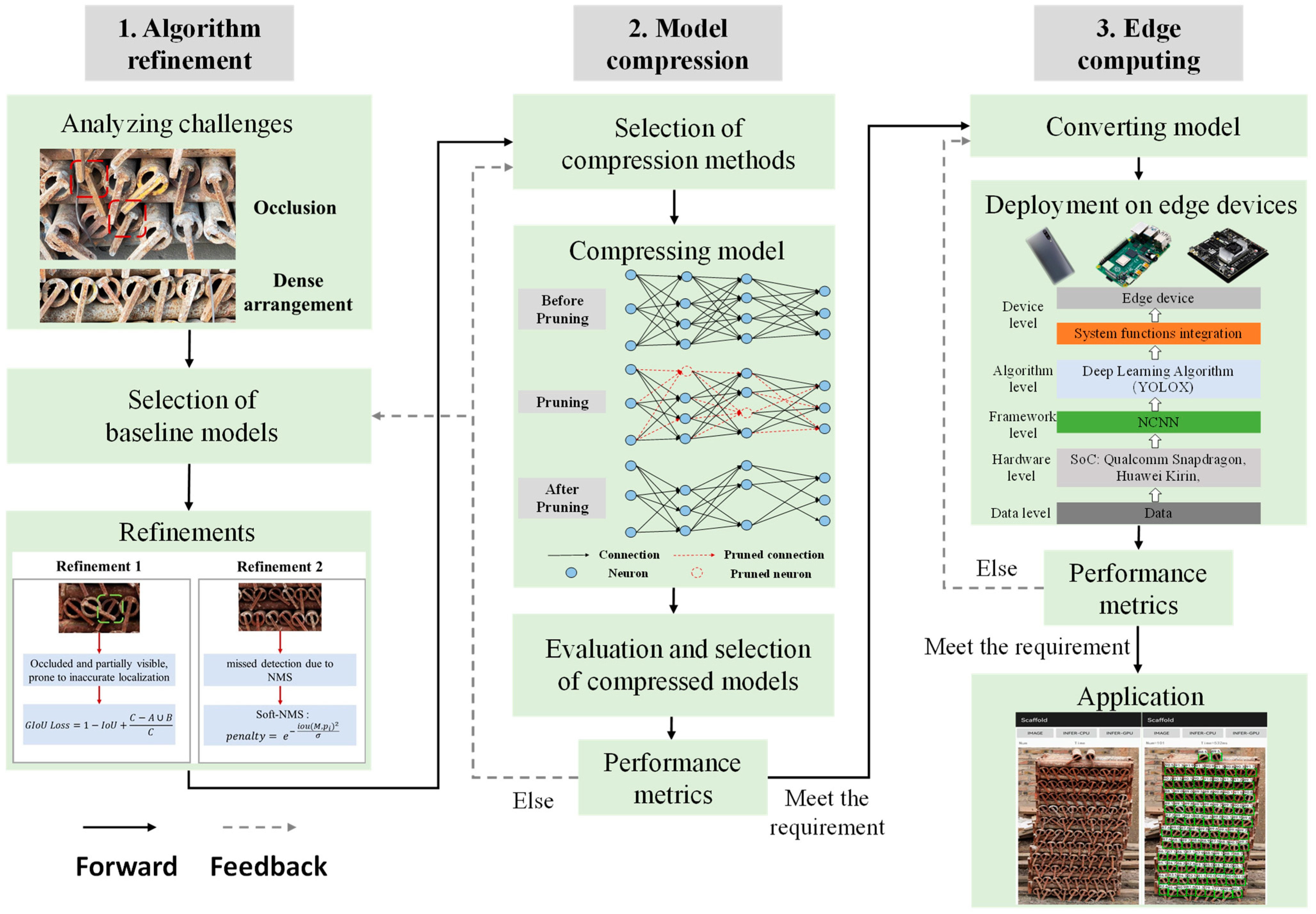
3.1. Overview of Workflow

The approach proposed in this study is depicted in Figure 2. It is composed of three interconnected segments—algorithm refinement, model compression, and edge computing—along with the flow of information between these segments. The framework encompasses the following steps:
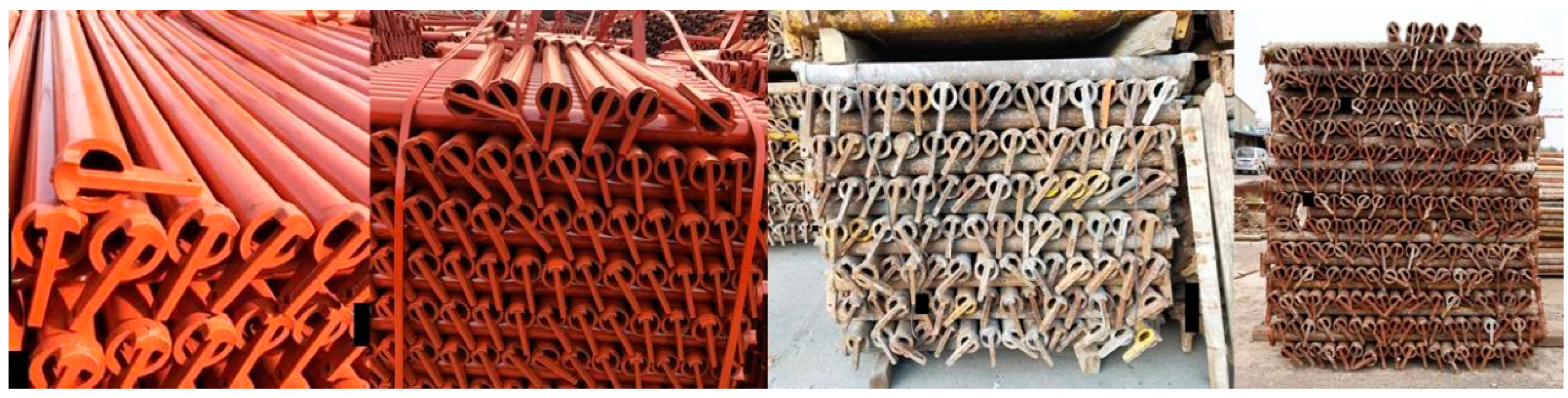
  • Challenge Analysis: Examine the characteristics of the tasks to identify the challenges and issues. For scaffold counting, the primary challenges are occlusion and dense arrangement.
  • Baseline Model Selection: Choose a baseline model that essentially aligns with the real-time and accuracy requirements of the tasks.
  • Algorithm Refinement: Propose a series of algorithmic refinements to address the identified challenges. Refined modules can range from pre-processing and post-processing algorithms to network architecture, loss function, and training strategies.
  • Compression Method Selection: Decide on the method for model compression. Options include network pruning, knowledge distillation, quantization, etc.
  • Execute Model Compression: Compress the refined model.
  • Model Evaluation: Evaluate the compressed models and select the most appropriate one based on the performance metrics.
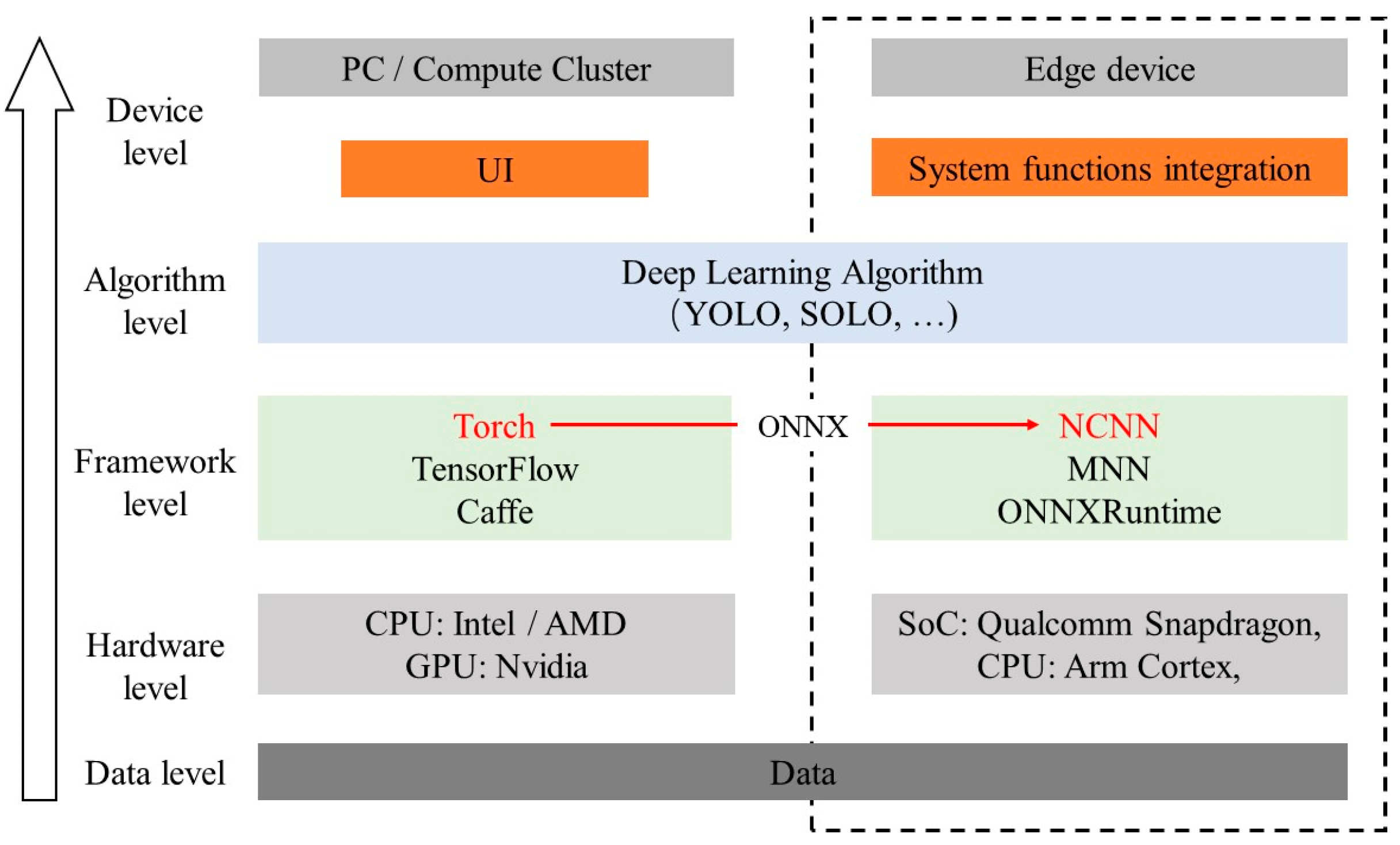
  • Model Conversion: Convert the selected model into a format that is compatible with edge devices.
  • Model Deployment: Deploy the model on the edge devices, integrating functionalities like data collection, pre-processing, post-processing, and model computing.
  • Application: Incorporate visualization and interaction functionalities on the edge device for enhanced user experience and interaction.
Beyond the steps mentioned above, the flow of information between different segments is a vital component of the framework. The forward information flow ensures the implementation of the whole method, while feedback information guides adjustments in the segments to obtain better performance.

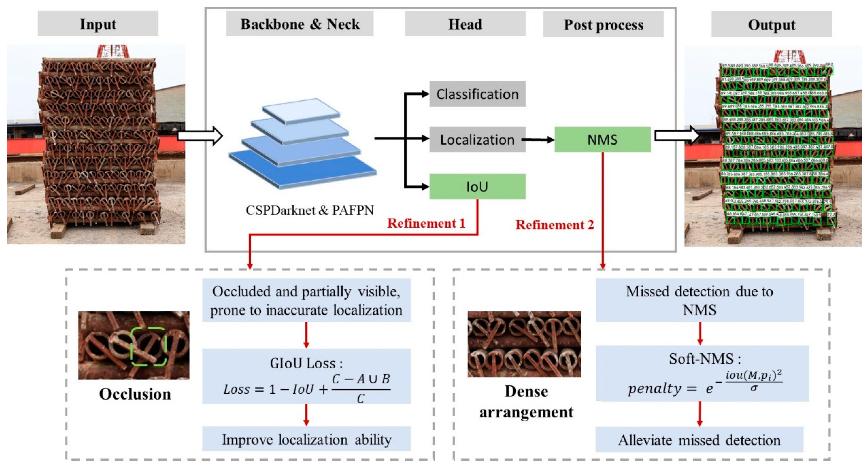
3.2. Algorithm Refinement

To address the challenges of occlusion and dense arrangement in scaffold tubes, two significant algorithmic refinements are introduced: generalized intersection over union (GIoU) and soft non-maximum suppression (Soft-NMS). This study selects the YOLOX [33] detector for its high speed and accuracy as the baseline model. As shown in Figure 3, YOLOX incorporates CSPDarknet as its backbone and PAFPN as the neck. It features a decoupled head, specifically engineered to resolve the inherent conflict between classification and regression tasks found in the YOLO series. This design distinctly separates three branches: classification, localization, and IoU. For the post-processing stage, non-maximum suppression (NMS) is employed to eliminate superfluous predictions.
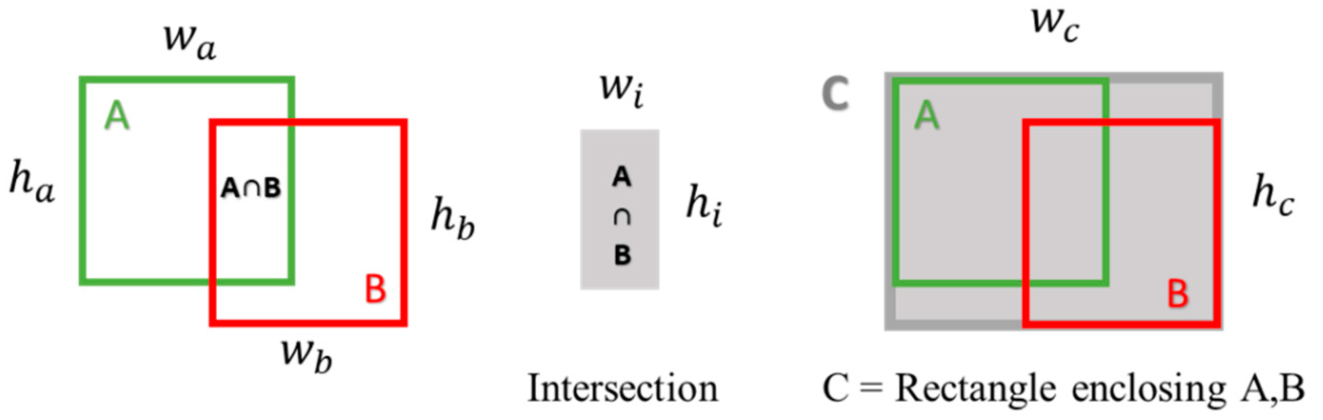
  • Generalized intersection over union (GIoU)
The original loss function of YOLOX is the IoU loss. For two areas A and B, the definition of IoU, as shown in Equation (1), is the intersection over union, where A∩B represents the intersection of the two areas, and A∪B denotes their union. The limitation of employing IoU as a loss function is its relatively weak capacity to quantify the spatial separation between A and B. For instance, in scenarios where A and B do not overlap, the IoU loss consistently remains at 1 and the gradient of the loss stabilizes at 0, regardless of the extent of their separation. This aspect highlights that IoU is insufficient for effective distance measurement between A and B, and this drawback leads to poor localization ability for targets.
To address the issue, this paper introduces GIoU [34], defined in Equation (3), where C represents the smallest enclosing rectangle bounding both A and B, as shown in Figure 4. GIoU enhances the original IoU by incorporating a penalty term related to the distance between areas A and B, expressed as (C − A∪B)/C. This term more effectively quantifies the relative distance. Furthermore, employing GIoU as a loss function mitigates the issue of gradient vanishing in IoU, thereby bolstering the model’s performance for detection and counting.
IoU = A B A B = h i w i h a w a + h b w b h i w i
IoU   Loss = 1 IoU
GIoU = IoU C A B C = h i w i h a w a + h b w b h i w i h c w c h a w a h b w b + h i w i h c w c
GIoU   Loss = 1 GIoU
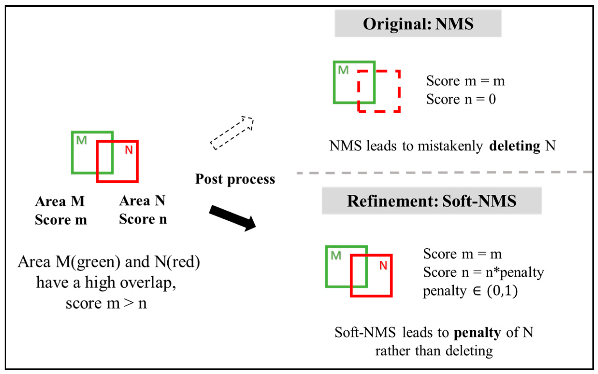
  • Soft non-maximum suppression (Soft-NMS)
The dense arrangement and occlusion of scaffold tubes can lead to a significant challenge for detection algorithms: overlapping predictions, or ‘overlapping bounding boxes’, as illustrated in Figure 5. Such overlaps often result in predictions being erroneously discarded by non-maximum suppression (NMS), the original post-processing algorithm utilized by YOLOX. This deletion of prediction boxes is not a desired outcome, as it can lead to potential missed detection. To address this issue without increasing computational cost, this study introduces Soft-NMS [35] as a substitute for the traditional NMS algorithm. When overlapping of prediction boxes occurs, Soft-NMS introduces a penalty factor to reduce the scores of the prediction boxes rather than eliminating them outright. This strategy significantly reduces the likelihood of erroneously deleting boxes, which, in turn, minimizes missed detections and enhances the overall performance of the detection and counting model.
Algorithm 1 illustrates the implementation process of Soft-NMS, wherein the penalty function, f ( M , p i ) , can be either a linear or a Gaussian function. In our study, a Gaussian function is employed, and its form is as follows:
f M , p i = e IoU ( M , p i ) 2 σ
Algorithm 1: Soft-NMS
Input P = { p 1 , p 2 , , p i } , S = { s 1 , s 2 , , s i } , f
P is the list of initial predictions
S contains the confidence score of every prediction i
f is the penalty function for Soft-NMS
Output: R is the result after Soft-NMS
S contains the confidence score of every prediction after Soft-NMS
1: S
2: while P is not empty do
3:  m arg max ( S )
4:  M p m
5:  R R M
6:  P P M
7: for p i in P do
8:   f M , p i e IoU ( M , p i ) 2 σ
9:   s i s i f M , p i
10: end for
11: end while
12: return R , S

3.3. Model Compression

This research proposes an automated network pruning method to speed up the enhanced model. Network pruning typically involves four steps: determining pruning parameters, executing pruning, retraining model, and performance evaluation. These steps require cumbersome operations, making the application of pruning challenging. To achieve network pruning automatically and efficiently, this study innovates by automating the typical steps of model pruning, retraining, and performance evaluation via a script. In contrast to conventional pruning methods, which require manual execution, the presented method is efficient and easy to use, which consists of the following 4 steps:
  • Determination of Pruning Hyperparameters.
  • Weight Assessment and Branch Elimination.
  • Retraining.
  • Performance Evaluation.
Algorithm 2 outlines the pseudocode necessary for the implementation of this automated pruning method. Leveraging this methodology, the research further explores the impacts of varying the pruning factor λ. By adjusting λ and repeating the entire pruning process, models with different levels of compression can be efficiently generated and evaluated.
Algorithm 2: Pruning
Input Ω = { c 1 , c 2 , , c i } , W = { w 1 , w 2 , , w n } , λ [ 0 , 1 ]
Ω is the list of network structures to be pruned
W contains all the weights of network structures
λ is the pruning factor
Output: Performance metrics is the evaluation result of pruned network
1: r a n k S o r t W , a s c e n d i n g _ o r d e r
2: while Ω is not empty do
3:  for c i in Ω do
4:    k i r a n k ( c i )
5:   if k i < n λ then
6:     R R c i
7:     Ω Ω c i
8:   end if
9:  end for
10: end while
11: retrain network with structure Ω
12:  Performance   metrics E v a l u a t i o n ( network Ω )
13: return Performance metrics
With the pruning method, a series of compressed models can be obtained by different pruning factors λ. From these models, the most suitable one must be selected for deployment on edge devices. The challenge lies in how to evaluate a series of compressed models and select an optimal (or approximately optimal) one for deployment. This problem can be transformed into an optimization problem under various constraints. The key metric, algorithm accuracy (AP), is selected as the optimization objective. Other performance metrics, such as inference speed, computing power (measured in giga floating point operations per second, GFLOPs), the number of model parameters, and runtime memory, are considered constraints. This optimization problem is formulated as Function (6). The optimization problem can be addressed through methods like mathematical programming and heuristic algorithms.
argmax λ   p e r f o r m a n c e ( AP , AR ) s . t .   inference   speed > r 1 computing   power < r 2 model   parameters < r 3 runtime   memory < r 4

3.4. Model Deployment on Edge Devices

The edge-computing-driven approach for scaffold tube counting can be implemented through model converting and deployment. Model converting refers to the process of transforming models, which were trained, refined, and compressed on servers or computers, into formats compatible with edge devices. Typically, deep learning models developed for execution on standard computing hardware, such as desktop computers, workstations, and computing clusters, are not inherently compatible with edge devices. To bridge this gap, a conversion process is necessitated. Open Neural Network Exchange [36] (ONNX) emerges as a critical tool in this context. ONNX offers an open-source format that facilitates the conversion of models into an architecture suitable for various platforms and environments. In our research, ONNX is utilized to transform the models into a format that is compatible with the NCNN framework [37], a high-performance framework optimized for edge devices, as shown in Figure 6.
For the model deployment, the study emphasizes an edge-dominant computing strategy to guarantee quick response. This necessitates a comprehensive integration of all operational modules, including data collection, pre-processing, model inference, post-processing, results visualization, and user interaction. To achieve this integration, the study employs Android Studio, a widely used development environment for building Android applications. By using Android Studio, we successfully amalgamate all these functionalities into a singular, cohesive application. As a result, the entire process, from data input to visualization of results, is streamlined to function efficiently and autonomously on the edge device.

4. Experiments

4.1. Dateset and Devices

The dataset utilized in this research is a specialized collection of scaffold images, consisting of 907 images featuring approximately 165,901 scaffold tubes. The dataset encompassed five distinct construction sites with deliberate variations in lighting conditions (dawn/dusk, full daylight, cloudy), camera perspectives (different angles, 0.5–10 m working distances), and structural complexity (2–13 scaffold layers, partial/complete stacked). The size of these images varies, ranging from 500 to 1300 pixels. To facilitate accurate model training, each image in the dataset was meticulously annotated with bounding box information. These annotations were stored in two prominent formats: COCO format [38] and VOC format [39], ensuring compatibility and ease of use across different training frameworks. A selection of images from this dataset is presented in Figure 7 to provide visual insights into the data characteristics.
For the training of the detection model, this study employed the PyTorch 1.7 framework. The hardware setup for this task included a robust 48-core Intel® Xeon® Gold 5220R CPU operating at 2.20 GHz and a high-performance GeForce RTX 3090 GPU. The dataset was strategically divided into a training set and a testing set, following a 7:3 ratio, to ensure a balanced approach to model learning and validation. In pursuit of enhancing the diversity and robustness of the training data, the study applied various data augmentation techniques. These techniques included mosaic augmentation [40], hue, saturation, value (HSV) enhancement, and random flipping. These methods were crucial in creating a more varied and comprehensive training dataset, leading to improved model performance. However, it was noted through testing that the mixup data augmentation technique [41] did not yield significant benefits in the context of scaffold tube counting and was consequently not incorporated into our training process.
For the deployment phase on edge devices, this study selected two widely used smartphones with robust specifications: the HUAWEI P30, equipped with a Kirin980 System on Chip (SoC) and 8 GB RAM, and the XIAOMI MIX2S, featuring a SnapDragon845 SoC and 6 GB RAM.

4.2. Performance Metrics

The metrics applied in this study were of two types: accuracy and efficiency.
(1)
Accuracy
Accuracy is the most commonly used metric for counting methods, defined as
Accuracy = 1 F P + F N G T
where false positive (FP) denotes the number of false detections, false negative (FN) denotes the number of missed detections, and ground truth (GT) is the total amount of entities.
Another performance metric is average precision (AP), which is defined as
AP = r = 0 1 p ( r )   a t   IoU = 0.50 : 0.05 : 0.95
where p ( r ) is the maximum precision at recall r , and the intersection over union (IoU) threshold increases from 0.50 to 0.95 with a step of 0.05.
AP @ α = r = 0 1 p ( r )   a t   IoU = α
AP @ α measures the average precision at a fixed IoU threshold of α . In this study, AP @ 50 (coarse metric) and AP @ 75 (strict metric) are used.
(2)
Efficiency
Inference time measures the inference speed of the model. Normally this metric is defined as the average time consumption of multiple inference tests.
inference   time = 1 N i = 1 N t ( i )
Network parameters are the total parameters of the model, and this metric is calculated as
Network   parameters = j l a y e r s p a r a m ( j ) for   each   CNN   layer ,   p a r a m = C o u t ( k w k h C i n + 1 )
where p a r a m j is the parameters of layer j, C o u t and C i n are the numbers of output channels and input channels, k w and k h are the width and height of the kernel.
The total computation amount is measured by floating point operations (FLOPs) of a network, defined as:
Network   FLOPs = k l a y e r s FLOPs ( k ) for   each   CNN   layers ,   FLOPs = 2 H W ( C i n k w k h + 1 ) C o u t
where F L O P s k is the FLOPs of layer k, W and H are the width and height of the input feature map, C o u t and C i n are the number of output channels and input channels, k w and k h are the width and height of the kernel.

5. Results

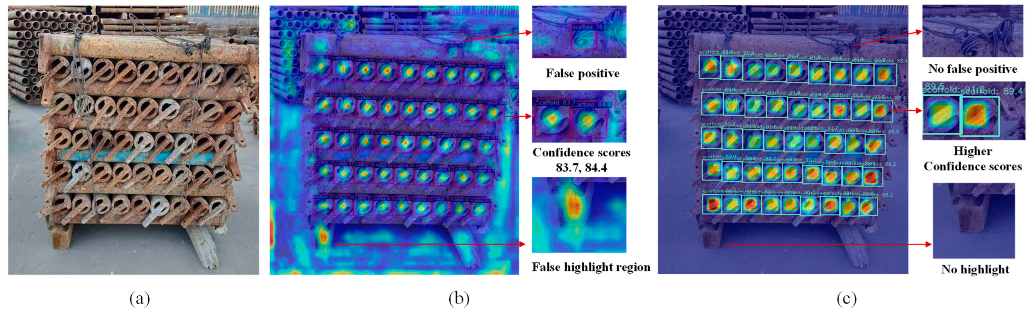
5.1. Results of Scaffold Detection

To evaluate the impact and efficacy of the two proposed algorithmic refinements, this study designed a structured ablation experiment. The results of this experiment are summarized in Table 3. The baseline for comparison is the performance metrics of the original YOLOX model, as detailed in the table’s second row. This serves as a reference point to understand the incremental benefits brought about by each refinement. In the experiment’s third row, the performance outcomes following the incorporation of Soft-NMS into YOLOX are presented. This refinement leads to a slight improvement in the average precision (AP) of the model, indicating its positive effect on detection accuracy. The fourth row of the table displays the performance after enhancing the original model with the GIoU loss function. This modification results in a more pronounced increase in the model’s AP, signifying its substantial contribution to improving detection accuracy. Furthermore, the fifth row combines both algorithmic refinements—Soft-NMS and GIoU loss function. Here, the results demonstrate that the synergy of these enhancements maximizes the AP performance of the model, outstripping the individual contributions of each refinement. Moreover, as indicated by the inference time column, there is a negligible change in the inference time before and after algorithmic refinement, suggesting that the refinements have almost no negative impact on the inference speed.
To validate the superior performance of our improved YOLOX model in terms of accuracy and inference time, a comparative experiment with different detection methods, including Faster R-CNN [42], SSD [43], YOLOv5 [44], and YOLOv7 [45], was performed. To ensure fairness and objectivity, the input image size was fixed at 960 pixels, though it is important to note that SSD only supports inputs of 512 pixels due to its inherent algorithmic constraints. The findings from this comparative experiment are detailed in Table 4. These results show that our improved YOLOX algorithm not only achieves higher average precision (AP and AP@50) but also demonstrates a reduction in inference time compared to its counterparts.

5.2. Results of Model Compression and Deployment

With the automated network pruning method delineated in Section 3.3, a series of compressed models were obtained, each with its corresponding performance metrics. Table 5 shows the metrics for both the original model A and the ultimately adopted model D. The pruning factor λ = 0 for model A indicates no pruning, with the results serving as a reference. The computing power demand for model A is 59.93 GFLOPs, which equals 59.93 × 10⁹ floating point operations, and the model has 8.94 million parameters. This model is more suitable for running on professional computers, as the computational burden is heavy for edge devices, resulting in poor real-time inference performance. When pruning factor λ scales from 0 to 0.375, the model size decreases by 60.9% (from 8.94 M to 3.50 M parameters), GFLOPs drop by 60.2%, and inference time decreases by 8.4%, enabling the model to meet deployment requirements. However, the average precision (AP) only decreased by a modest 3.9%. This analysis indicates that the pruning method substantially reduces the model’s parameter and computational cost, and accelerates inference speed, without significant loss of model accuracy.
For deployment, the edge devices used in this study were the HUAWEI P30 and XIAOMI MIX2S. Deploying the model on these edge devices for scaffolding tube count tests, the results revealed that the size of the model on the edge devices was only 39.1 MB, with an inference speed per image ranging from 400–800 ms, with an accuracy of 98.8%. Note that all computations were executed by the edge device during the counting task.

6. Discussion

6.1. The Rationale for Improved Algorithm

To provide a clearer understanding of the efficacy and logic behind the algorithmic improvements implemented in this research, this study utilized Grad-CAM [46] for generating visual explanations for the models before and after improvement. Grad-CAM is a visual explanation tool that works by creating heat maps of the input images, indicating which parts of the images were pivotal for the predictions of the model. The heat maps of two models, the original YOLOX and our improved version, were generated using Grad-CAM. As shown in Figure 8, the original YOLOX model demonstrated issues with false positives and incorrect attention allocation. In contrast, the improved model rectified these errors, while achieving higher confidence scores for the target objects (i.e., scaffold tubes). The results from the visual explanations substantiate that our algorithmic refinements have indeed enhanced the model’s performance.
This study also attempts to theoretically analyze the effectiveness of using GIoU instead of IoU as the loss function. Figure 9 demonstrates two cases of these loss functions. In both scenarios, regions A and B have the same width and height l . The line charts, depicting the variation of GIoU and IoU losses with the change in horizontal distance x , are plotted. The following findings were observed:
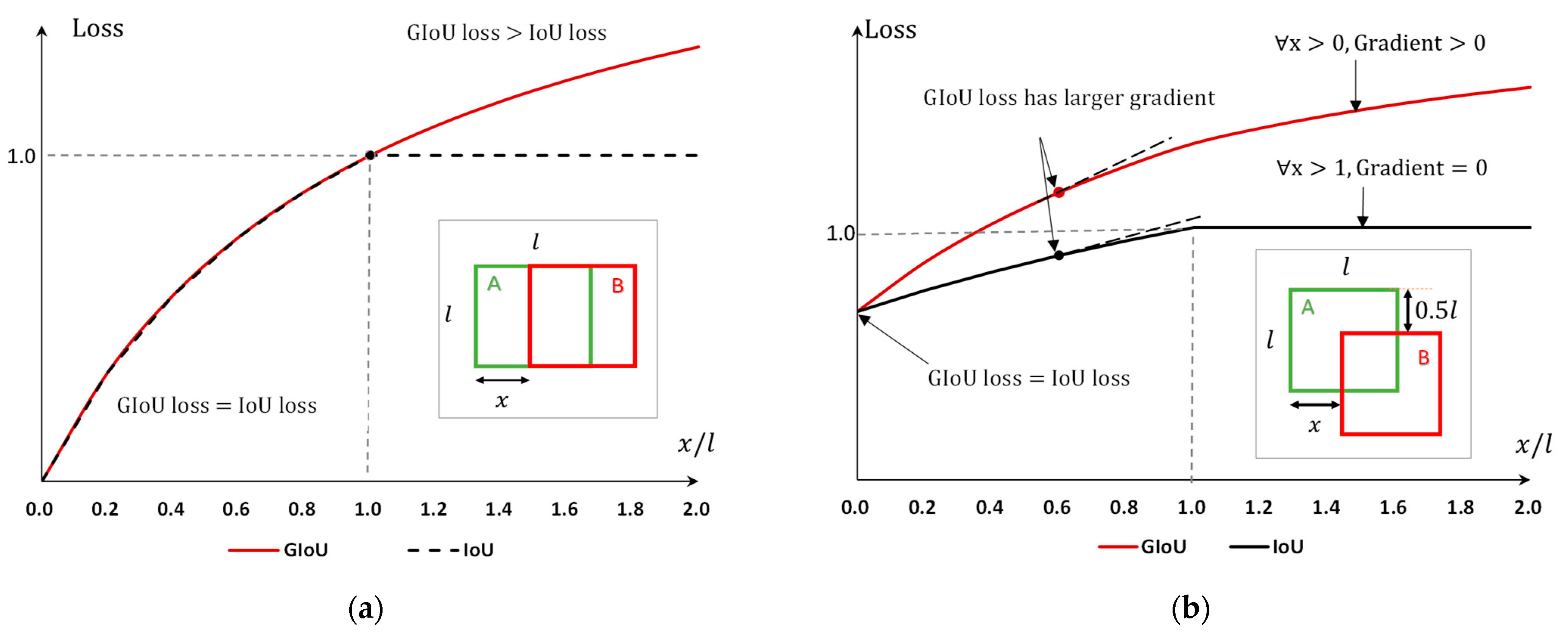
  • GIoU loss ≥ IoU loss. GIoU loss always serves as an upper bound for IoU loss. This implies that the GIoU loss provides a more comprehensive error measurement by considering both the overlap and the relative positions.
  • Greater gradient in GIoU loss. In the second case, the gradient of the GIoU loss is larger compared to that of the IoU loss. This larger gradient is beneficial for the convergence of the training process, as it provides a stronger correction signal for the model when the prediction is far from the actual target.
  • Non-zero gradient for GIoU. When x > l (i.e., when there is no overlap between the two areas), the IoU loss remains at 1, leading to a zero gradient. In such cases, optimization using IoU loss becomes infeasible since the loss function fails to provide a direction for improvement. In contrast, the gradient of GIoU loss remains greater than zero even in these scenarios, ensuring continuous optimization potential.
From these findings, it is evident that GIoU offers advantageous features for the training process, particularly in situations where traditional IoU fails to provide valid gradients for optimization. Therefore, GIoU is a superior choice for a loss function in detection models, enhancing both the accuracy and efficiency of training.

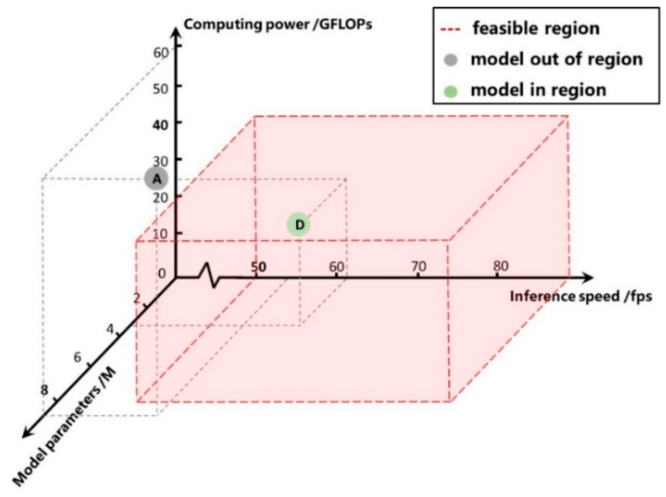
6.2. Optimal Selection of Compressed Models

This section aims to explore how to select a compressed model. Based on the automated network pruning method introduced in Section 3.3, we have derived multiple compressed models and assessed their performance metrics, as detailed in Table 6. Additionally, Section 3.3 reformulates the selection of models into an optimization problem, subject to constraints such as inference speed and computing power. In line with the practical engineering needs of the scaffold tube counting, the constraints were specifically set as an inference speed exceeding 50 fps, computing power less than 40 GFLOPs, and model parameters below 8 million. This optimization problem is outlined as follows:
argmax λ   AP s . t .   i n f e r e n c e   s p e e d > 50 f p s c o m p u t i n g   p o w e r < 40 G F L O P s m o d e l   p a r a m e t e r s < 8 M
We solve this problem using mathematical programming techniques. The solution space and the feasible region of this issue can be visualized in a three-dimensional space. Figure 10 displays the solution space across three dimensions: model parameters, inference speed, and computing power, with the feasible region marked by a red dashed line. The eight models from Table 6 are projected into this space, represented by solid circles, where grey circles denote models whose performance metrics fall outside the feasible region, and green indicates models within it. Models A and D, for instance, were visualized in the solution space, with model A out of the feasible region while D was inside of it. Integrating Figure 10 with the mathematical model, model D, having the highest AP within the feasible region, is selected as the optimal solution through our mathematical programming approach.

6.3. Generalization Across Unseen Scenarios

To evaluate the generalization capacity of the proposed methodology, we conducted comprehensive validation experiments using completely unseen data from a new construction site containing 249 scaffold components, which was explicitly excluded from the original training dataset. As illustrated in Figure 11, this testing environment presents particularly challenging operational conditions characterized by severe backlighting effects and suboptimal illumination levels. Despite these adverse conditions, the proposed model achieved a mean average precision of 76.3% in scaffold component detection. Notably, the system exhibited complete absence of false negatives or false positives in the unseen scenarios. These empirical results substantiate the model’s robust generalization capabilities across diverse real-world construction environments, particularly in handling complex lighting variations that commonly impair visual detection systems.

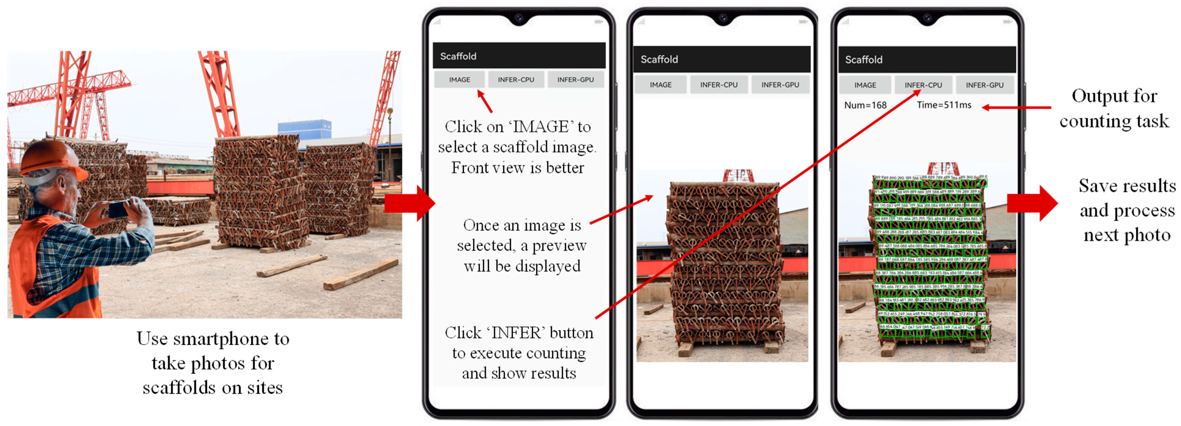
6.4. Field Application
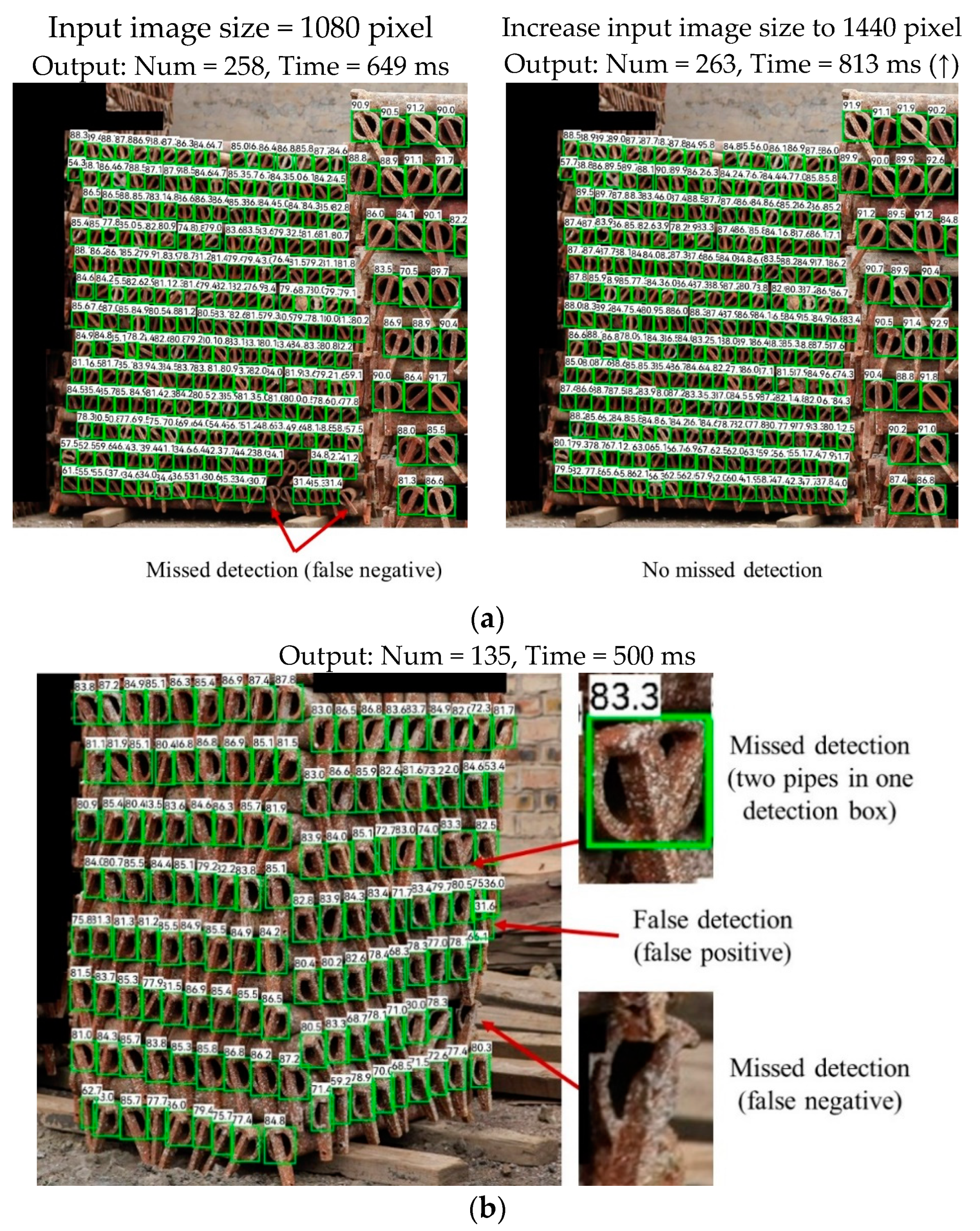
Building upon the research conducted in this study, we have designed and developed a scaffold tube counting application. The guideline of this application is illustrated in Figure 12. With this application, users can finish counting tasks with several clicks of buttons. To reveal the efficiency and accuracy of our counting application, we conducted scaffold tube counting tasks in two construction projects in China. For the proposed automated counting method, a single worker operated the edge-computing-driven system to complete the entire counting task. In parallel, two workers collaboratively performed counts of the scaffold components for comparison. The total manual counting time was calculated as the sum of both workers’ completion times. The project information and statistical results are displayed in Table 7. The results show that, in a residential building project with a total area of approximately 35,225.2 m2, about 34,650 scaffold tubes were used throughout the construction process. Each scaffold tube has to be counted when entering and leaving the construction site, totaling 69,300 counts. If performed manually, this task would take about 8.09 h, equivalent to the workload of 2–3 workers. In contrast, using the application presented in this study required less than one hour, reducing the workload by 87.9%, significantly alleviating the workers’ burden while also achieving higher accuracy. In another field test conducted at a bridge project site, similar conclusions were drawn: for the same scaffold tube counting task, the method proposed in this paper not only demonstrated higher accuracy compared to manual effort but also saved 86.9% in terms of time consumption.
The case studies reveal that the method proposed in this paper can be applied for the rapid and accurate counting of scaffold tubes in various scenarios such as production, transportation, usage, and storage. Compared to manual counting, this method can save a considerable amount of time, substantially reducing both labor and time costs.
Compared to existing studies [2,3,5], our approach integrates a novel pruning method and edge computing optimization, and the model size decreases by 60.9%, FLOPs drop by 60.2%, and inference time decreases by 8.4%. These optimizations substantially reduce computational overhead while accelerating detection speed. Crucially, the proposed method maintains high practical performance, achieving 98.8% counting accuracy for scaffold on site. This balance between precision and efficiency eliminates manual verification requirements, reducing labor costs by approximately 86% (based on time consumption) and enabling rapid, scalable material management.
Beyond the scaffold tube counting case, the method proposed in this paper can be applied to various materials. The algorithmic improvements, including the GIoU loss function and the Soft-NMS post-processing algorithm, are particularly effective for objects with dense occlusions, such as rebar, bricks, and timber. Additionally, the approach is not only suitable for deploying detection algorithms to edge devices but also applicable to other algorithms for tasks like object classification, pose estimation, and semantic segmentation. Researchers can leverage the methodologies outlined in this paper to utilize edge devices for sophisticated applications in construction sites, such as posture analysis, progress management, and structural health monitoring.
This study presents methods that support a wide range of edge devices. These methods enable researchers to deploy our models across various platforms through model conversion, encompassing devices such as smartphones, tablets, Raspberry Pi, drones, and VR/AR devices. With the widespread availability of high-performance smart devices, the edge computing paradigm emerges as a significant enabler for innovative and intelligent applications within the architecture, engineering, and construction (AEC) sector.

6.5. Limitations

During practical applications, certain limitations of our counting method have been identified, mainly reflected in two aspects: (1) an excessive number of small targets in the image can result in missed detections; (2) side-view images may lead to missed and false detections. Figure 13 demonstrates two cases of these issues.
  • Case 1
In Case 1, the image contains a total of 263 scaffold tubes. Using the proposed method, 258 targets were successfully detected, with five missed and no false detections. The accuracy is 98.1%, and the whole process took 0.649 s. The visualization results are shown in Figure 13a, where five tubes at the bottom of the image were missed. The analysis suggests that the possible reason for this error is the small target size of the scaffold tubes, which contain few pixels, leading to a detection confidence level below the threshold and ultimately resulting in missed detections. To verify this viewpoint, the resolution of the same input image was increased to 1440 pixels, so that each scaffold tube could contain more pixels. We saw a significant improvement in the accuracy of counting results, with no missed detections in the outcomes. However, this adjustment also increased the computation time from 0.649 s to 0.813 s. This case reveals a trade-off between the accuracy and the computation time in this study.
  • Case 2
Case 2, shown in Figure 13b, demonstrates the outcome of photographing scaffolds from a side view. The total number of scaffold tubes is 136. The method identified 135 targets, with two missed and one false detection. The accuracy was calculated at 97.8%, and the process was completed in 0.5 s. The results indicated that the majority of the scaffold tubes were successfully detected, but missed detections and false positives occurred on the far right of the image. The reason for this is that the tubes on the extreme right were severely occluded from a side view, making their shape and contours difficult to recognize, leading to missed detections and false positives. To avoid such issues, it is recommended to shoot scaffolds from the front view when using the proposed method. When shooting from the side view, the tilt angle should not be too large.
Despite some limitations of the method described in this study, it remains capable of achieving rapid and accurate scaffold counting in most scenarios. During practical on-site tests, the overall error rate was maintained below 1.5%, which is deemed acceptable. More critically, the method significantly reduces the time required for scaffold counting, offering a faster and more accurate alternative compared to existing methods.

7. Conclusions

Scaffold tube counting is a tough task on construction sites and there is a need for counting scaffold components accurately and swiftly. This study proposed an edge computing-driven approach based on the YOLOX detector for both accurate and swift scaffold counting. Firstly, two algorithm refinements for YOLOX were introduced to improve accuracy under occlusion scenarios. Secondly, an automated pruning method was proposed to accelerate the model. Then the counting model was deployed on edge devices to guarantee quick response. Finally, comparative studies and two practical case studies were performed. The conclusions can be drawn as follows:
  • The proposed approach effectively achieves accurate and rapid scaffold tube counting on edge devices, demonstrating an accuracy rate of 98.8% and a latency ranging from 0.4 to 0.8 s per image.
  • The introduction of two algorithmic refinements enhanced the mean average precision by 5.3% (from 72.3% to 77.6%), without increasing the inference time. The improved YOLOX outperformed other state-of-the-art detectors in scaffold detection and counting.
  • The implementation of an automated pruning method streamlined the compression process. This approach resulted in a 60.2% reduction in computational demand and a 9.1% increase in inference speed, with no significant compromise in accuracy.
Our study contributes to the research field from two aspects. (1) An enhanced counting method is proposed to improve accuracy in occlusion scenarios. (2) An automated pruning method is proposed to efficiently compress and accelerate the counting model. Additionally, the proposed method inherently supports functional extensibility through its modular architecture. By collecting domain-specific data from additional construction materials (e.g., steel tubes, rebars) and performing lightweight finetuning—such as adjusting partial network layers and leveraging a pruning method—the model can efficiently adapt to new material counting tasks.
While this study acknowledges its contributions, it also identifies limitations. First, the vision-based approach may exhibit compromised performance in scenarios where images are captured from suboptimal viewing angles, potentially leading to inaccurate component detection. Second, the heterogeneity of edge computing devices introduces uncertainties in model adaptability, particularly regarding variations in detection accuracy, energy efficiency, and robustness under harsh environmental conditions (e.g., extreme weather, dust interference). Third, the influence of diverse model compression techniques—such as quantization, knowledge distillation, and neural architecture search (NAS)—on system performance remains insufficiently characterized.
To address these challenges, future research will focus on three key directions:
  • Multi-sensor fusion for enhanced robustness. The framework could integrate 2D images and RFID tag signals through a multi-sensor fusion mechanism to address occlusion and environmental interference in material management. This cross-modal alignment compensates for limitations in single sensing modalities—for instance, RFID provides spatial identity under low visibility, while visual data resolve tag collisions.
  • Edge device performance benchmarking. Systematic evaluations of edge devices will be conducted to quantify their impacts on model accuracy, computational latency, energy consumption, and environmental resilience. This analysis will inform hardware selection and optimization strategies for real-world deployment.
  • Model compression technique optimization. A comparative study will assess how advanced compression methods—including but not limited to quantization-aware training, teacher–student distillation, and NAS—affect the trade-off between model efficiency and accuracy performance. The findings will guide the development of lightweight yet accurate models for edge computing platforms.
These extensions aim to advance the robustness, generalizability, and practicality of edge-computing-driven solutions for construction material management.

Author Contributions

Conceptualization, X.Z. and B.C.; methodology, B.C.; software, B.C.; validation, B.C.; formal analysis, Y.L. and Z.H.; investigation, B.C.; resources, X.Z.; data curation, B.C.; writing—original draft preparation, B.C.; writing—review and editing, Y.L. and Z.H.; visualization, B.C.; supervision, X.Z.; project administration, X.Z.; funding acquisition, X.Z. and Y.L. All authors have read and agreed to the published version of the manuscript.

Funding

This research was funded by the National Key Research & Development Program of China (2022YFC3801700), Chinese Academy of Engineering (2024-XZ-37), Fundamental Research Funds for the Central Universities (2024-1-ZD-02, 22120240236), Science and Technology Commission of Shanghai Municipality (22dz1207100), Shanghai Qi Zhi Institute (SQZ202309).

Data Availability Statement

The data presented in this study are available on request.

Acknowledgments

The authors acknowledge Glodon Company Limited for their support in terms of data collection.

Conflicts of Interest

The authors declare no conflicts of interest.

Abbreviations

The following abbreviations are used in this manuscript:
GIoUGeneralized intersection over union
Soft-NMSSoft non-maximum suppression
NMSNon-maximum suppression
FLOPsFloating point operations
GFLOPsGiga Floating Point Operations per Second
HSVHue, saturation, value
FPFalse positive
FNFalse negative
GTGround truth
APAverage precision
ONNXOpen Neural Network Exchange

References

  1. Hou, L.; Zhao, C.; Wu, C.; Moon, S.; Wang, X. Discrete Firefly Algorithm for Scaffolding Construction Scheduling. J. Comput. Civ. Eng. 2017, 31, 04016064. [Google Scholar] [CrossRef]
  2. Wang, H.; Polden, J.; Jirgens, J.; Yu, Z.; Pan, Z. Automatic Rebar Counting using Image Processing and Machine Learning. In Proceedings of the 2019 IEEE 9th Annual International Conference on CYBER Technology in Automation, Control, Suzhou, China, 29 July–2 August 2019, and Intelligent Systems (CYBER); pp. 900–904.
  3. Li, Y.; Lu, Y.; Chen, J. A deep learning approach for real-time rebar counting on the construction site based on YOLOv3 detector. Autom. Constr. 2021, 124, 103602. [Google Scholar] [CrossRef]
  4. Xiang, Z.; Rashidi, A.; Ou, G. An improved convolutional neural network system for automatically detecting rebar in GPR data. In Proceedings of the ASCE International Conference on Computing in Civil Engineering, Atlanta, GA, USA, 17–19 June 2019; American Society of Civil Engineers: Reston, VA, USA, 2019; pp. 422–429. [Google Scholar]
  5. Han, K.K.; Golparvar-Fard, M. Appearance-based material classification for monitoring of operation-level construction progress using 4D BIM and site photologs. Autom. Constr. 2015, 53, 44–57. [Google Scholar] [CrossRef]
  6. Lauer, A.P.R.; Benner, E.; Stark, T.; Klassen, S.; Abolhasani, S.; Schroth, L.; Gienger, A.; Wagner, H.J.; Schwieger, V.; Menges, A.; et al. Automated on-site assembly of timber buildings on the example of a biomimetic shell. Autom. Constr. 2023, 156, 105118. [Google Scholar] [CrossRef]
  7. Li, Y.; Chen, J. Computer Vision–Based Counting Model for Dense Steel Pipe on Construction Sites. J. Constr. Eng. Manag. 2022, 148, 04021178. [Google Scholar]
  8. Katsigiannis, S.; Seyedzadeh, S.; Agapiou, A.; Ramzan, N. Deep learning for crack detection on masonry façades using limited data and transfer learning. J. Build. Eng. 2023, 76, 107105. [Google Scholar]
  9. Davis, P.; Aziz, F.; Newaz, M.T.; Sher, W.; Simon, L. The classification of construction waste material using a deep convolutional neural network. Autom. Constr. 2021, 122, 103481. [Google Scholar]
  10. Han, Q.; Liu, X.; Xu, J. Detection and Location of Steel Structure Surface Cracks Based on Unmanned Aerial Vehicle Images. J. Build. Eng. 2022, 50, 104098. [Google Scholar] [CrossRef]
  11. Kamari, M.; Ham, Y. Vision-based volumetric measurements via deep learning-based point cloud segmentation for material management in jobsites. Autom. Constr. 2021, 121, 103430. [Google Scholar]
  12. Beckman, G.H.; Polyzois, D.; Cha, Y.-J. Deep learning-based automatic volumetric damage quantification using depth camera. Autom. Constr. 2019, 99, 114–124. [Google Scholar] [CrossRef]
  13. Wang, P.; Yan, Z.; Han, G.; Yang, H.; Zhao, Y.; Lin, C.; Wang, N.; Zhang, Q. A2E2: Aerial-assisted energy-efficient edge sensing in intelligent public transportation systems. J. Syst. Archit. 2022, 129, 102617. [Google Scholar] [CrossRef]
  14. Habib, M.; Bollin, E.; Wang, Q. Edge-based solution for battery energy management system: Investigating the integration capability into the building automation system. J. Energy Storage 2023, 72, 108479. [Google Scholar] [CrossRef]
  15. Akhavian, R.; Behzadan, A.H. Smartphone-based construction workers’ activity recognition and classification. Autom. Constr. 2016, 71, 198–209. [Google Scholar] [CrossRef]
  16. Abner, M.; Wong, P.K.-Y.; Cheng, J.C.P. Battery lifespan enhancement strategies for edge computing-enabled wireless Bluetooth mesh sensor network for structural health monitoring. Autom. Constr. 2022, 140, 104355. [Google Scholar] [CrossRef]
  17. Maalek, R.; Lichti, D.D.; Maalek, S. Towards automatic digital documentation and progress reporting of mechanical construction pipes using smartphones. Autom. Constr. 2021, 127, 103735. [Google Scholar]
  18. Chen, C.; Gu, H.; Lian, S.; Zhao, Y.; Xiao, B. Investigation of Edge Computing in Computer Vision-Based Construction Resource Detection. Buildings 2022, 12, 2167. [Google Scholar] [CrossRef]
  19. Chen, K.; Zeng, Z.; Yang, J. A deep region-based pyramid neural network for automatic detection and multi-classification of various surface defects of aluminum alloys. J. Build. Eng. 2021, 43, 102523. [Google Scholar] [CrossRef]
  20. Wang, N.; Zhao, X.; Zhao, P.; Zhang, Y.; Ou, J. Automatic damage detection of historic masonry buildings based on mobile deep learning. Autom. Constr. 2019, 103, 53–66. [Google Scholar]
  21. Alexander, Q.G.; Hoskere, V.; Narazaki, Y.; Maxwell, A.; Spencer, B.F., Jr. Fusion of thermal and RGB images for automated deep learning based crack detection in civil infrastructure. AI Civ. Eng. 2022, 1, 3. [Google Scholar]
  22. Kizilay, F.; Narman, M.R.; Song, H.; Narman, H.S.; Cosgun, C.; Alzarrad, A. Evaluating fine tuned deep learning models for real-time earthquake damage assessment with drone-based images. AI Civ. Eng. 2024, 3, 15. [Google Scholar]
  23. Cheng, Y.; Wang, D.; Zhou, P.; Zhang, T. A Survey of Model Compression and Acceleration for Deep Neural Networks. arXiv 2017, arXiv:1710.09282. [Google Scholar]
  24. Cheng, J.; Wang, P.S.; Gang, L.I.; Qing-Hao, H.U.; Han-Qing, L.U. Recent advances in efficient computation of deep convolutional neural networks. Front. Inf. Technol. Electron. Eng. 2018, 19, 64–77. [Google Scholar] [CrossRef]
  25. Lecun, Y. Optimal Brain Damage. Neural Inf. Proceeding Syst. 1990, 2, 598–605. [Google Scholar]
  26. Hassibi, B.; Stork, D.G. Second order derivatives for network pruning: Optimal brain surgeon. In Proceedings of the 6th International Conference on Neural Information Processing Systems, San Francisco, CA, USA, 30 November–3 December 1992; pp. 164–171. [Google Scholar]
  27. Guo, Y.; Cui, H.; Li, S. Excavator joint node-based pose estimation using lightweight fully convolutional network. Autom. Constr. 2022, 141, 104435. [Google Scholar]
  28. Wu, P.; Liu, A.; Fu, J.; Ye, X.; Zhao, Y. Autonomous surface crack identification of concrete structures based on an improved one-stage object detection algorithm. Eng. Struct. 2022, 272, 114962. [Google Scholar]
  29. Gong, Y.; Liu, L.; Yang, M.; Bourdev, L. Compressing Deep Convolutional Networks using Vector Quantization. arXiv 2014, arXiv:1412.6115. [Google Scholar]
  30. Hinton, G.; Vinyals, O.; Dean, J. Distilling the Knowledge in a Neural Network. Comput. Sci. 2015, 14, 38–39. [Google Scholar]
  31. Chen, Z.; Yang, J.; Chen, L.; Feng, Z.; Jia, L. Efficient railway track region segmentation algorithm based on lightweight neural network and cross-fusion decoder. Autom. Constr. 2023, 155, 105069. [Google Scholar]
  32. Hong, Y.; Chern, W.-C.; Nguyen, T.V.; Cai, H.; Kim, H. Semi-supervised domain adaptation for segmentation models on different monitoring settings. Autom. Constr. 2023, 149, 104773. [Google Scholar] [CrossRef]
  33. Ge, Z.; Liu, S.; Wang, F.; Li, Z.; Sun, J. YOLOX: Exceeding YOLO Series in 2021. arXiv 2021, arXiv:2107.08430. [Google Scholar]
  34. Rezatofighi, H.; Tsoi, N.; Gwak, J.; Sadeghian, A.; Reid, I.; Savarese, S. Generalized Intersection Over Union: A Metric and a Loss for Bounding Box Regression. In Proceedings of the 2019 IEEE/CVF Conference on Computer Vision and Pattern Recognition (CVPR), Long Beach, CA, USA, 15–20 June 2019; pp. 658–666. [Google Scholar]
  35. Bodla, N.; Singh, B.; Chellappa, R.; Davis, L.S. Improving Object Detection with One Line of Code. arXiv 2017, arXiv:1704.04503. [Google Scholar]
  36. ONNX. Open Neural Network Exchange. Available online: https://github.com/onnx/onnx (accessed on 28 April 2022).
  37. NCNN. A High-Performance Neural Network Inference Framework Optimized for the Mobile Platform. Available online: https://github.com/Tencent/ncnn (accessed on 28 April 2022).
  38. Lin, T.-Y.; Maire, M.; Belongie, S.; Hays, J.; Perona, P.; Ramanan, D.; Dollár, P.; Zitnick, C.L. Microsoft COCO: Common Objects in Context; Fleet, D., Pajdla, T., Schiele, B., Tuytelaars, T., Eds.; Computer Vision—ECCV 2014; Springer International Publishing: Cham, Switzerland, 2014; pp. 740–755. [Google Scholar]
  39. Everingham, M.; Eslami, S.M.A.; Van Gool, L.; Williams, C.K.I.; Winn, J.; Zisserman, A. The Pascal Visual Object Classes Challenge: A Retrospective. Int. J. Comput. Vis. 2015, 111, 98–136. [Google Scholar] [CrossRef]
  40. Bochkovskiy, A.; Wang, C.-Y.; Liao, H.-Y.M. Yolov4: Optimal speed and accuracy of object detection. arXiv 2020, arXiv:2004.10934. [Google Scholar]
  41. Zhang, H.; Cisse, M.; Dauphin, Y.N.; Lopez-Paz, D. mixup: Beyond Empirical Risk Minimization. arXiv 2017, arXiv:1710.09412. [Google Scholar]
  42. Ren, S.; He, K.; Girshick, R.; Sun, J. Faster R-CNN: Towards Real-Time Object Detection with Region Proposal Networks. IEEE Trans. Pattern Anal. Mach. Intell. 2017, 39, 1137–1149. [Google Scholar] [CrossRef]
  43. Berg, A.C.; Fu, C.Y.; Szegedy, C.; Anguelov, D.; Erhan, D.; Reed, S.; Liu, W. SSD: Single Shot MultiBox Detector. arXiv 2015, arXiv:1512.02325. [Google Scholar]
  44. U. LLC. YOLOv5. 2020. Available online: https://github.com/ultralytics/yolov5 (accessed on 28 April 2022).
  45. Wang, C.-Y.; Bochkovskiy, A.; Liao, H.-Y.M. YOLOv7: Trainable bag-of-freebies sets new state-of-the-art for real-time object detectors. In Proceedings of the IEEE/CVF Conference on Computer Vision and Pattern Recognition, Vancouver, BC, Canada, 17–24 June 2023; pp. 7464–7475. [Google Scholar]
  46. Selvaraju, R.R.; Cogswell, M.; Das, A.; Vedantam, R.; Parikh, D.; Batra, D. Grad-CAM: Visual Explanations from Deep Networks via Gradient-Based Localization. In Proceedings of the 2017 IEEE International Conference on Computer Vision (ICCV), Venice, Italy, 22–29 October 2017. [Google Scholar]
Figure 1. Plug-attached scaffold tubes. (a) Illustration of scaffold components. (b,c) Stacked scaffold tubes. (d) Characteristic: dense arrangement. (e) Characteristic: occlusion. This study is dedicated to effective counting of such components.
Buildings 15 01190 g001
Figure 2. Workflow of the proposed approach.
Buildings 15 01190 g002
Figure 3. Network architecture of YOLOX and our refinements.
Buildings 15 01190 g003
Figure 4. Illustration of Intersection and Union of A, B.
Buildings 15 01190 g004
Figure 5. Illustration of Soft-NMS for post-processing. The green square frames represent bounding box M, while the red frames represent bounding box N.
Buildings 15 01190 g005
Figure 6. Framework for deployment on the edge and other devices.
Buildings 15 01190 g006
Figure 7. Images from the scaffold dataset.
Buildings 15 01190 g007
Figure 8. Heat maps generated by Grad-CAM. (a) Input image. (b) Original YOLOX. (c) Our improved YOLOX.
Buildings 15 01190 g008
Figure 9. Comparison of GIoU loss and IoU loss. A and B represent two regions where loss needs to be calculated (a) Case 1: the vertical distance between A and B is zero. (b) Case 2: the vertical distance between A and B equals 0.5 l .
Buildings 15 01190 g009
Figure 10. Illustration of solution space and feasible region.
Buildings 15 01190 g010
Figure 11. Generalization across unseen scenarios. (a) Backlighting condition; (b) insufficient illumination.
Buildings 15 01190 g011
Figure 12. Practical application guideline.
Buildings 15 01190 g012
Figure 13. Two cases of missed detection and false detection. (a) Case 1: missed detection due to small target size; (b) Case 2: errors due to side-view image.
Buildings 15 01190 g013
Table 1. Types of strategy in edge computing.
Type of StrategyData
Collection
Data Processing & AnalyzingResult & FeedbackReferenceAdvantageDisadvantage
Cloud-dominantEdgeCloudCloud[2,4,9,11,12,19]High computing power,
extensibility
Data loss,
bandwidth pressure
Cloud–edge
collaboration
EdgeCloudEdge[3,7,14,15,16,17,20,21]High computing power,
extensibility
Data loss,
bandwidth pressure,
high latency
Edge-dominantEdgeEdgeEdge[18,22]Quick response,
data security,
convenience
Low computing power,
limited accuracy
Table 2. Computing power index of different devices.
DeviceTypeComputing Power Index
Windows computer
(i7-RTX3090)
Professional computer100
MacBook Pro
(M2 Pro)
Personal computer19
Huawei Mate40 pro
(Kirin9000)
Smartphone/Edge device18
iPhone14
(A16)
Smartphone/Edge device12
Jetson-TX1
(Cortex-A57)
Minicomputer/Edge device4
Raspberry Pi-4B
(Cortex-A72)
Minicomputer/Edge device1
Note: Device with RTX3090 is selected as reference for computing power index, with larger index value indicating better computing ability.
Table 3. Ablation experiment of YOLOX detector for scaffold tube detection.
YOLOXAP/%AP@50/%AP@75/%Inference Time/ms
Baseline72.391.589.517.9
+Soft-NMS73.0 (+0.7)92.9 (+1.4)90.0 (+0.5)18.1
+GIoU77.4 (+5.1)95.6 (+4.1)93.6 (+3.1)18.3
+GIoU and Soft-NMS77.6 (+5.3)95.9 (+4.4)93.9 (+3.4)17.8
Table 4. Comparative experiment of different detectors for scaffold tube detection.
ModelBackboneAP/%AP@50/%Inference Time/ms
Faster R-CNNResNet5073.191.161.1
SSDVGG1663.278.251.8
YOLOv5CSP-Darknet5377.192.923.0
YOLOv7ELAN77.293.121.9
YOLOX-GIoU and Soft-NMSCSP-Darknet5377.695.917.8
Table 5. Results of model compression.
Model RefPruning FactorAP/%Params/MComputing Power/GFLOPsInference Time/ms
A (unpruned)077.68.9459.9317.8
D0.37574.6
(↓3.9%)
3.50
(↓60.9%)
23.86
(↓60.2%)
16.3
(↓8.4%)
The arrows indicate the trend of change. Note: The Inference time data were obtained on a professional computer with RTX3090. It is not possible to test inference speed on edge devices because of high computing burden.
Table 6. Performance of the compressed models.
Model RefThree-Dimensional SpaceInside of Feasible RegionPerformance
Params/MComputing Power/GFLOPsInference Speed/fps AP/%
A8.9459.956.2No77.6
B6.8546.158.8No73.9
C5.0334.158.5Yes72.5
D3.5023.961.3Yes74.6
E2.2415.559.5Yes73.1
F1.268.960.2Yes71.0
G0.564.164.9Yes70.5
H0.141.172.5Yes67.8
Table 7. Two practical studies for scaffold counting.
Project InformationManualOur Method
IDTypeTotal Area
/m2
Number of ScaffoldsTotal CountTotal Time
/h
Accuracy
%
Total Time
/h
Accuracy
%
1Residential building35,225.2 34,65069,3008.09 98.50.98
(↓87.9%)
98.9
(↑0.4%)
2Bridge6375.725,50051,0005.95 98.10.78
(↓86.9%)
98.8
(↑0.7%)
The arrows indicate the trend of change.
Disclaimer/Publisher’s Note: The statements, opinions and data contained in all publications are solely those of the individual author(s) and contributor(s) and not of MDPI and/or the editor(s). MDPI and/or the editor(s) disclaim responsibility for any injury to people or property resulting from any ideas, methods, instructions or products referred to in the content.

