Performance-Based Design Assessment of a Chilean Prescriptive R.C. Shear Wall Building Using Nonlinear Static Analysis

Abstract

Performance-based seismic design (PBD) has emerged as a key approach for rationalizing prescriptive code provisions and improving the explicit assessment of structural performance. In Chile, where reinforced concrete shear wall buildings are the predominant structural typology, evaluating their seismic response beyond traditional linear methodologies is crucial. This study assesses the seismic performance of a representative Chilean shear wall residential building using the ACHISINA manual’s performance-based seismic design framework. A nonlinear static (pushover) analysis is performed to verify compliance with prescribed design criteria, incorporating capacity design principles and a moment envelope approach to prevent premature yielding in upper stories. The results confirm that the building meets the performance objectives for both Immediate Occupancy and Additional Deformation Capacity limit states. The application of capacity design effectively controls shear demand, preventing brittle failure, while the flexural design ensures the formation of the yielding mechanism (plastic hinge) at the intended critical section. Additionally, the study highlights the limitations of pushover analysis in capturing higher-mode effects and recommends complementary nonlinear time-history analysis (NLTHA) for a more comprehensive assessment. The computed response reduction factors exceed those used in the prescriptive design, suggesting a conservatively safe approach in current Chilean practice. This research reinforces the need to integrate performance-based methodologies into Chilean seismic design regulations, particularly for shear wall structures. It provides valuable insights into the advantages and limitations of current design practices and proposes improvements for future applications.

1. Introduction

Performance-based design emerged from the need to rationalize code provisions, which, although developed on an empirically validated basis through research and expert discussions, fail to explicitly demonstrate objective performance within the typical structural design process. Similarly, there is a need for a methodological framework that allows for the evaluation and demonstration of the feasibility of using innovative materials, architectural designs that exceed prescriptive limits—such as maximum building height—and/or structures with irregularities [1,2], among other cases, to the competent entities responsible for project review.

Moreover, decision-makers require a framework to assess the potential benefits of investing in a structure with enhanced seismic resistance, taking into account the expected damage and losses incurred throughout its service life. Additionally, societal needs regarding safety and potential losses during high-intensity earthquakes must also be considered, highlighting the objective of improving resilience against such events.

Although the theoretical foundation of performance-based design has been studied for several decades, as will be further explained in the following section, its application has become more feasible in recent years due to technological advancements, particularly in computational capacity, allowing for the development of more complex analytical models. Furthermore, ongoing research has led to the formulation of procedures and analysis methods that facilitate the transition from prescriptive methodologies to a more precise and explicit evaluation of the seismic behavior of structures.

In practice, seismic design codes in various countries have typically relied on linear response analysis, followed by the aforementioned prescriptive considerations. Chile is no exception, despite being a country with high seismic demand, where structures may undergo significant nonlinear response excursions.

This can be justified by the Chilean practice of structuring buildings using reinforced concrete shear walls as both gravitational and seismic-resistant elements, while also incorporating beams and slab lintels as coupling elements. In particular, it is common to use multiple wall segments with complex geometries, generally covering approximately 0.1% of the total area of all floors above the base level of the building in each direction. The effect of this configuration can be measured using performance indices such as the ultimate roof drift and the fundamental period relative to the building height, ${\displaystyle \frac{{\delta }_u}{H_o}}$ and ${\displaystyle \frac{H_o}{T}}$, respectively, which allow for the correlation between stiffness and deformation capacity [3,4,5].

Another factor that must be considered in structural design is the regulatory provisions for seismic design, particularly the interstory drift limits established by the Chilean code NCh433 [6], which provide considerable stiffness to the lateral load-resisting system. Additionally, due to changes in regulations prompted by the observed performance during the 2010 Maule earthquake [7,8,9,10], deformation capacity in shear walls is now verified by considering a roof displacement ${\delta }_u$ calibrated to the demands observed during that event. This has led to the prescriptive application of limits and specific detailing of boundary elements to ensure the necessary ductility. These advancements have enabled the implicit fulfillment of the Life Safety performance objective by achieving, through design, sufficient ductility in seismic-resistant elements, ensuring good performance under recurrent seismic events, and limiting structural damage due to high stiffness [4,5,11].

However, despite the validation of good performance in recent seismic events, there remains a need to develop a methodology that explicitly validates Chilean structural design practices. To address this, in 2017, the document “performance-based seismic design” [12] was introduced, providing guidelines for a more sophisticated analysis and design approach for buildings based on recent advancements in structural civil engineering. This document explains nonlinear static and dynamic analysis methods used to evaluate the Immediate Occupancy limit state of a structure under a Design Earthquake (DE), and a Collapse Prevention limit state under a Maximum Considered Earthquake (MCE).

Within this context, the seismic performance of a Chilean residential building designed according to Chilean regulations will be assessed using the ACHISINA manual [12], incorporating into the design the moment envelope and the capacity design for shear criteria. The objective is to verify the good performance of Chilean structures through a more advanced analysis that accounts for nonlinear structural excursions, identifies critical zones, evaluates seismic performance, and prevents the over-dimensioning of structural elements.

The results indicate that the structure, designed in accordance with Chilean regulations, meets the requirements of the Chilean performance-based design manual. It is observed that when performing a linear analysis considering capacity design and applying an overstrength factor, the shear demand does not exceed the value calculated by the method. Similarly, when applying the criterion of considering a moment envelope along the height, yielding of the upper stories is prevented due to moment redistribution once plastic hinging occurs in the critical section at the base. Furthermore, it is confirmed that the structure exhibits ductile behavior and a response reduction factor greater than that used in the linear design.

To achieve the stated objective and provide better context for the methodological framework used, it is necessary to review the state of the art of the performance-based design method, which will be addressed in the following section.

2. Performance-Based Design Background

2.1. First Developments of Performance-Based Design

The concepts underlying the performance-based design method have been incorporated into the provisions of various structural design codes, where the expected performance levels have been qualitatively defined since the 1960s [13]. These levels include the following:

• Minor seismic events without damage.
• Moderate seismic events, potentially sustaining damage in non-structural elements.
• Major seismic events, equal to the most severe historical earthquake experienced, prevent collapse while sustaining both structural and non-structural damage.

However, during this period, it was recognized that there was insufficient knowledge to establish and define parameters for evaluating these performance levels. Consequently, an empirical methodology for linear force-based analysis was developed, incorporating coefficients to account for the effects of nonlinear excursions within the expected seismic behavior. Under this context, most seismic-resistant design codes were developed, where compliance with prescriptive regulations—validated through experimentation—aims to achieve a design that ensures either Life Safety or Collapse Prevention, ensuring ductility in elements expected to undergo inelastic behavior through proper detailing, while, for other elements, failure due to excessive forces is prevented.

In the 1970s, the displacement-based method was developed. Based on observations of dynamic performance in laboratory tests, a correlation between structural displacement response and experienced damage was identified. By the 1990s, this approach evolved into what is now known as the Direct Displacement-Based Design Method [14]. These advancements enabled the calculation of the ultimate displacement of structures, whether considering nonlinearity or not, making it a standard practice in seismic-resistant engineering. This shift led to a design approach where the expected damage is defined at the outset, which is a fundamental characteristic of performance-based design.

Another notable development during this period is the philosophy of capacity design. Although its concepts were introduced as early as the 1960s through various studies and research efforts, it reached maturity in the 1970s and gained global recognition through bibliographic publications in the 1990s [15,16] and later incorporated into future design codes. Under this design approach, brittle failure of structural elements is prevented by ensuring, through deterministic design, the development of a ductile failure mechanism (usually controlled by flexure).

Simultaneously, in the 1990s, the first generation of performance-based design guidelines began to emerge, primarily aimed at establishing a framework for structural performance assessment. This initiative was mainly driven by the need to evaluate the condition of existing buildings affected by seismic events, where the structural engineer—upon the request of the owner—had to determine the performance of an already constructed structure to assess whether rehabilitation was necessary or feasible. Additionally, for future projects, evaluating the economic feasibility of investing in a structure with enhanced seismic resistance—compared to the minimum prescriptive code requirements—became an area of interest. Among the most significant guidelines from this period are VISION 2000 [17], FEMA 273 [18], and ATC-40 [19]. Given the limited scope of the article, they are not reviewed in detail. For readers interested in further exploring these documents, the following references provide an in-depth review of their contents [20,21].

2.2. Modern Guidelines

Through the first-generation guidelines, the foundations of the performance-based design method were established. In particular, the procedures introduced by FEMA 273 [18] significantly increased interest in nonlinear analysis within professional practice. It is important to emphasize that while this document was primarily developed for the rehabilitation of existing buildings, this did not prevent its application in the design of new structures. In many cases, this approach was used to achieve improved performance or, alternatively, to obtain an equivalent performance level at a lower cost, particularly in high-rise buildings.

Due to this growing interest and the gap in guidelines for the design of new structures, new publications were developed to integrate and standardize recent research through expert consensus. These efforts were further supported by technological advancements, enabling the development of more complex computational analyses. Among these publications, the most notable are EN-1998-1 [22], EN-1998-3 [23], ASCE 7 [24], ASCE/SEI-41 [25], TBI [26], and LATBSDC [27], which will be discussed in the following sections. However, a comprehensive review of their content is beyond the scope of this document; therefore, interested readers are encouraged to consult the following references [28,29,30,31].

2.2.1. ASCE 7-22

The following document was developed by the American Society of Civil Engineers (ASCE) with the primary objective of determining minimum loads and load combinations for structural design. This includes the determination of seismic hazard levels, which, when combined with material-specific provisions, allow for the design of new structures following established standards.

The most recent version of the standard, ASCE 7 [24], not only governs typical prescriptive design but also includes provisions for performance-based design, as presented in section 1.3 of this standard. For this purpose, the document provides guidelines for conducting a Response History Analysis (RHA), detailed in chapter 16, which was developed based on FEMA 273 [18]. The analysis incorporates seismic hazard levels, specifically the Design Basis Earthquake (DBE) and the Maximum Considered Earthquake (MCE). The DBE is primarily used to determine the structure’s stiffness, while the MCE is used to verify its stability, ductility, and force demands for elements classified as deformation- or force-controlled, respectively.

2.2.2. ASCE/SEI 41

As part of the standardization process of the previously mentioned guidelines, the publication of the ASCE standard under the name ASCE/SEI-41 [25] stands out, with its first edition released in 2006. Given that its contents are derived from FEMA 273 [18], its primary objective is to define the performance-based design method for the seismic evaluation of existing buildings. In its most recent edition, ASCE/SEI-41 [25], the document is closely interrelated with ASCE 7 [24], particularly in defining performance objectives, which include the Basic Performance Objective Equivalent to New Building Standards (BPON) and Enhanced Performance Objectives, corresponding to equivalent or superior performance levels, respectively. However, the standard acknowledges that existing buildings should not be evaluated using the same criteria as new buildings. Therefore, it introduces the Basic Performance Objective for Existing Buildings (BPOE), which establishes less stringent performance requirements for the same seismic hazard levels. For the BPON performance objective, for a building category I or II, hazards are defined according to ASCE 7 [24], considering either 2/3 $MC{E}_r$ for a Life Safety performance level and $MC{E}_r$ for a Collapse Prevention performance level. On the other hand, for the BPOE performance objective, it considers a hazard level of 20%/50 years for Life Safety performance level and 5%/50 years for a Collapse Prevention performance level.

2.2.3. PEER TBI and Alternative Procedure of LATBSDC

Due to the growing demand for high-rise buildings in the United States and the strict requirements imposed by design codes, performance-based design guidelines for this building category were developed. Notable among these are the following: “An Alternative Procedure for Seismic Analysis and Design of Tall Buildings”, developed by the Los Angeles Tall Building Structural Design Council (LATBSDC), and “Tall Building Initiative (TBI)”, developed by the Pacific Earthquake Engineering Research Center (PEER).

In this regard, an important aspect is that the ACHISINA manual [12] procedure is based on the LATBSDC document [27], in which the former defines different performance objectives: Immediate Occupancy for a Design Earthquake (SD) and Additional Deformation Capacity (comparable to Collapse Prevention in LATBSDC) for a Maximum Considered Earthquake (MCE). A notable similarity between the two methodologies is the allowance of nonlinear dynamic analysis, with ACHISINA manual [12] also permitting static pushover analysis for the Additional Deformation Capacity objective. Regarding acceptance criteria, both LATBSDC [27] and TBI [26] adopt the acceptance criteria from ASCE 41 [25]. However, LATBSDC aligns with the use of unit strain parameters for compression and tension in concrete and steel for reinforced concrete walls. Additionally, a key difference exists in global acceptance criteria, where interstory drift limits are defined in both documents (LATBSDC [27] and ACHISINA [12]) but with varying allowable values.

Table 1. Comparison between tall building and Chilean PBD guidelines.

		LATBSDC (2023) [27]	ACHISINA (2017) [12]
Performance objective	Performance level	Serviceability (SLE)	Immediate Occupancy
	Hazard level	50%/30 years, approximately equivalent to a return period of 43 years	Design Earthquake (SD), defined by design displacement spectrum or period of return of 475 years
	Global criteria	Interstory Drift: 0.5%	Interstory Drift: 0.5% and 0.7% for fragile and ductile non-structural elements, respectively
	Component criteria (walls)	ASCE 41 IO Acceptance Criteria hinge rotation for flexure controlled lateral translation for shear controlled	Strain limits: Unconfined concrete (compression): 0.3% Confined concrete (compression): 0.8% Reinforcement steel (tensile): 3%
Performance objective	Performance level	$\mathrm{Collapse}\mathrm{Prevention}\left(MC{E}_r\right)$	Additional Deformation Capacity
	Hazard level	$MC{E}_r$per ASCE 7	Maximum Considered Earthquake (MCE) by default, 30% greater displacement spectrum for SD or 950 period of return
	Global criteria	Loss in initial strength <20% Interstory Drift Transient: mean <3% peak <4.5% Residual: mean <1% peak <1.5%	Not applicable, checked implicitly by component criteria
	Component criteria (walls)	ASCE 41 CP Acceptance Criteria Additionally, LATBSDC recommends strain limits for flexure-controlled elements	Strain limits: Unconfined concrete (compression): 0.3% Confined concrete (compression): 1.5% Reinforcement steel (tensile): 5%

provides a comparison of the requirements between these documents.

Based on the above, the ACHISINA alternative procedure [12] can be regarded as an adaptation of the performance-based design method to Chilean engineering practice, integrating seismic hazard definitions, regulatory performance parameters, and societal expectations regarding building performance. This adaptation emphasizes Immediate Occupancy for Design-level earthquakes ($SD$) and Additional Deformation Capacity (comparable to Collapse Prevention) for a Maximum Considered Earthquake ($MCE)$, both based on the design displacement spectrum used in the Chilean code prescriptions.

2.3. Current Developments in Chilean Performance-Based Design

Even though Chile has had the ACHISINA procedure document since 2017, it is important to note that it is not yet officially standardized, and its use has been primarily limited to research applications and the review of high-rise buildings and/or structures with complex configurations. However, at the time of this article’s publication, several groups of professionals are actively working on the development of publications and updates to regulations relevant to this methodology, as listed below:

• Update of NCh433 [6] (Seismic Design of Buildings), which includes revisions to soil classification based on dynamic parameters (periods) and allows the performance-based design method as an alternative design approach.
• Update of NCh430 [32](Reinforced Concrete Design), which updates the referenced ACI 318 standard from the 2008 edition [33] to the 2019 edition [34]. Among various changes, this update incorporates capacity design principles.
• Development of the new NCh3792 [35] standard (performance-based seismic design), aimed at standardizing the methodology outlined in the ACHISINA [12] document for professional practice, as permitted under NCh433 [6].

3. Materials and Methods

3.1. Building, Material and Design Description

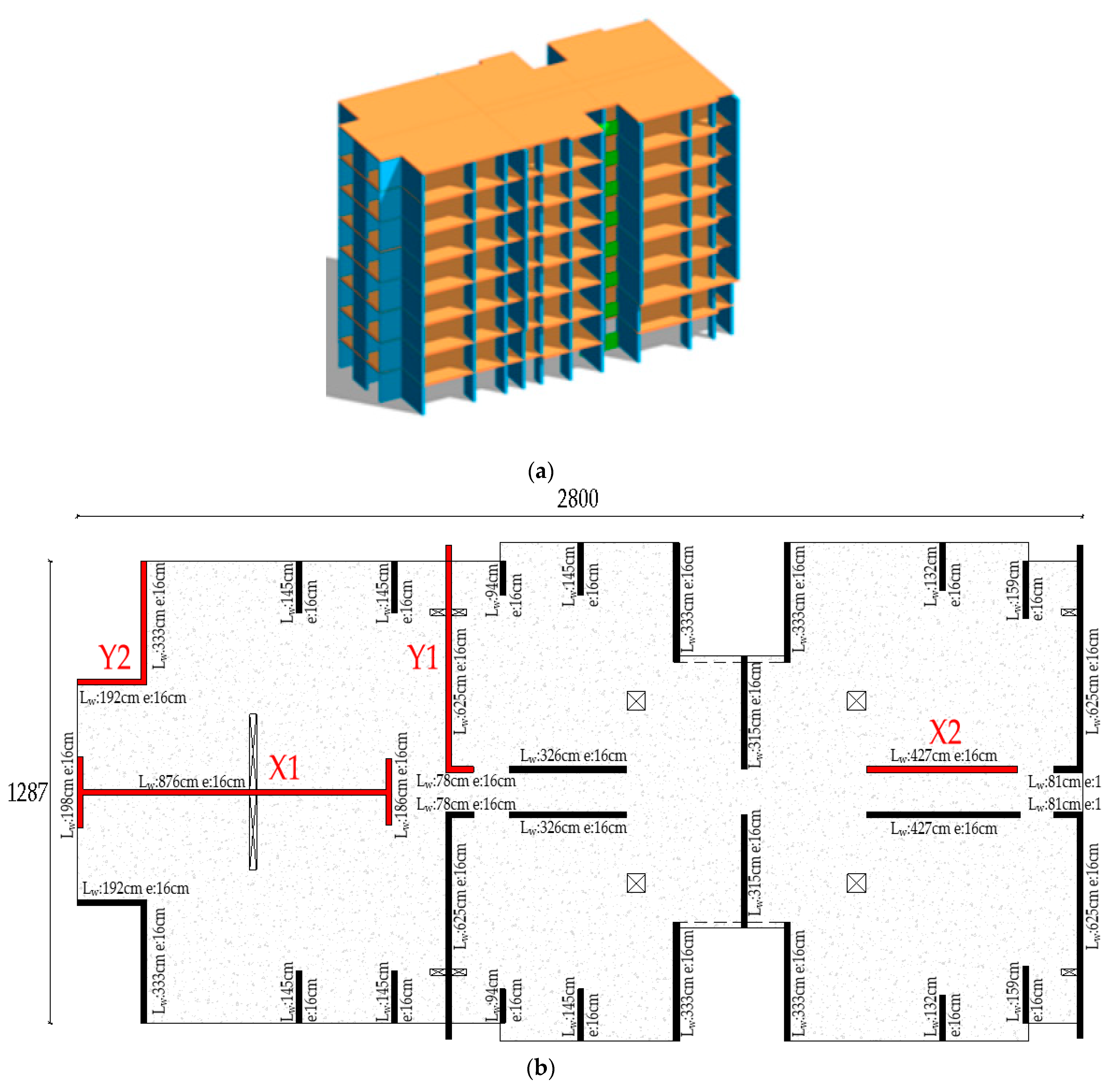
The analyzed building is a residential structure located in Seismic Zone 3 of Chile (effective acceleration = 0.4 g), situated on Soil Type B, according to the NCh433 code [6]. The intended use of the structure as a residential building classifies it as Category II, consisting of eight floors, each with a height of 2.52 m, except for the top floor, which has a height of 2.50 m, resulting in a total building height of 20.14 m. Each floor has a total plan area of 343 m².

Regarding its structural system, the building is composed of special reinforced concrete shear walls with a thickness of 16 cm, designed in accordance with Chilean regulations, which prescribes the following requirements to ensure ductile behavior:

• Limiting the shear wall slenderness by prescribing a minimum thickness $e\ge h/16$ where $h$ is the interstory height.
• Limiting the maximum compression in the shear wall to a maximum of $P_u\le 0.35f_c^{\prime }{A}_g$ where $f_c\prime$ and $A_g$ corresponds to the characteristic concrete resistance and gross section area, respectively.
• Special boundary elements (confinement) with a minimum thickness of $e\ge 30 \mathrm{cm}$ are required when the concrete compressive strain is ${\epsilon }_c\ge 0.3\%$ under the design roof displacement ${\delta }_u$.
• When special boundary elements are required, concrete compressive strain is limited to a maximum value of $0.8\%$ under the design roof displacement ${\delta }_u$.

The design of the structure is performed using a linear analytical model of the structure created using the commercial software ETABS (v2022) [36], where

• Walls and slabs are modeled as four-node shell elements.
• Beams, which in this specific case do not function as coupling elements, are modeled as two-node frame elements.
• The boundary condition at the base is assumed as fixed support.
• The horizontal force transfer system is explicitly modeled using the reinforced concrete slab, which is considered a rigid diaphragm.

Regarding the stiffness of the mathematical model, the Chilean code does not prescribe the use of a stiffness modifier to consider cracking in the concrete, using gross section properties instead. However, the following structure design criteria consider the ACI-318-08 [32] prescriptions in section 8.8.2, which specify 50% of the gross section properties, which represents the effect of cracking under the effects of a seismic event.

Regarding the loads applied to the model, dead and live loads are applied according to the Chilean regulation, which are summarized in Table 5.

To consider the seismic component for the design, modal spectral analysis is utilized, with the results summarized in

Table 2. Modal response spectral analysis results.

Parameter	X-Direction	Y-Direction
$\mathrm{Seismic}\mathrm{weight}(1D+0.25L$$\left)\right[\mathrm{k}\mathrm{N}]$	22,063.98
$\mathrm{Fundamental}\mathrm{period}\left[\mathrm{s}\right]$	0.50	0.375
$\mathrm{Response}\mathrm{reduction}\mathrm{factor}{R}^{*}$	7.64	6.85
$\mathrm{Elastic}\mathrm{base}\mathrm{shear}{Q}_{R=1}$$\left[\mathrm{k}\mathrm{N}\right]$	12,049.43	10,166.55
$\mathrm{Maximum}\mathrm{inelastic}\mathrm{base}\mathrm{shear}{Q}_{max}$$\left[\mathrm{k}\mathrm{N}\right]$	3089.09	3089.09
$\mathrm{Minimum}\mathrm{inelastic}\mathrm{base}\mathrm{shear}{Q}_{min}$$\left[\mathrm{k}\mathrm{N}\right]$	1470.99	1470.99
$\mathrm{Design}\mathrm{base}\mathrm{shear}{Q}_{design}$$\left[\mathrm{k}\mathrm{N}\right]$	1576.91	1483.75
$\mathrm{Inelastic}\mathrm{spectral}\mathrm{acceleration}{S}_a$$\left[{\mathrm{m}/\mathrm{s}}^2\right]$	0.96	1.42
$\mathrm{Inelastic}\mathrm{spectral}\mathrm{displacement}{S}_{de}$$\left[\mathrm{c}\mathrm{m}\right]$	4.9	3.5
$\mathrm{Computed}\mathrm{design}\mathrm{roof}\mathrm{displacement}{\delta }_u$$\left[\mathrm{c}\mathrm{m}\right]$	6.3	4.5
$\mathrm{Maximum}\mathrm{interstory}\mathrm{drift}\mathrm{in}\mathrm{CM}[\%]$	0.044	0.03
$\mathrm{Maximum}\mathrm{interstory}\mathrm{drift}[\%]$	0.005	0.045
Mode 1 period [s]	0.512	(Rotational)
Mode 2 period [s]	0.500	(Translational X)
Mode 3 period [s]	0.375	(Translational Y)
Mode 4 period [s]	0.135	(Translational X)

. The modal spectral analysis considers a design spectrum prescribed by the NCh433 [6] section §6.3.5.1, reduced to obtain the inelastic spectral acceleration ($S_a$), by a response reduction factor $R^{*}$ which is calculated according to section of §6.3.5.3, both dependent on the structure fundamental period and soil properties. A total of 11 modes are considered to comply with the 90% percentage of participating mass for the seismic action in both directions as required by NCh433 [6] section §6.3.3. These modes are then combined under CQC to obtain the maximum values in each direction; however, it is important to note that the standard does not prescribe the combination of direction effects in the seismic action. Subsequently, the standard limits the minimum ($Q_{min}$) and maximum $(Q_{max}$) value of base shear, as prescribed in section §6.3.7, which was not required to adjust for the structure under study. The design base shear ($Q_{design}$) considers the response reduction factor and the standard limits. Another parameter of interest is the design roof displacement (${\delta }_u)$, which is calculated as 1.3 times the displacement spectra ($S_{de}$) presented in the Supreme Decree DS61 [37], considering the aforementioned stiffness modifier under the effects of cracking. Finally, the building structure complies with the prescribed Center of Mass (CM) interstory drift limit of 0.2%, to ensure elevation regularity, and a maximum interstory drift of 0.1% (relative to the CM) for the plan regularity, as shown in Table 2.

Following these prescriptions, the walls are designed, which is shown in more detail in Section 3.2 of the following article. On the other hand, to evaluate the performance of the structural elements, four walls are selected in the following article for an in-depth analysis, see Figure 1. The building also includes reinforced concrete beams, shown in Figure 1 as dashed lines, commonly found in residential buildings, which serve as parapets for architectural purposes, with dimensions of 16 × 115 cm, as well as reinforced concrete slabs with a thickness of 15 cm.

Based on the parameters that relate stiffness to the deformation capacity of the building, according to the bio-seismic profile in Chile [3], the structure can be classified as rigid.

Regarding the materials, the concrete grade is G25 for both walls and beams, while the reinforcement steel used is A630-420H; the properties are listed in Table 6.

3.2. Element Design Description

A key aspect of the building is the design of the elements composing the seismic-resistant structure. For this purpose, the design follows current Chilean regulations, which require compliance with Supreme Decrees DS60 and DS61 [37,38], the former being a modification of the 2008 edition of the ACI 318 manual [33].

Within this framework, the critical section is designed by considering flexural demands for the Design Earthquake specified in NCh433 [6] and the ultimate roof displacement (${\delta }_u$) according to the values in Table 2, assuming that the critical section is located at the building’s base (first floor). It is important to emphasize that, due to the building’s characteristics—including its height, wall geometry, and seismic demand—it was not necessary to incorporate special boundary elements (confinement), as prescribed in Chilean regulations. 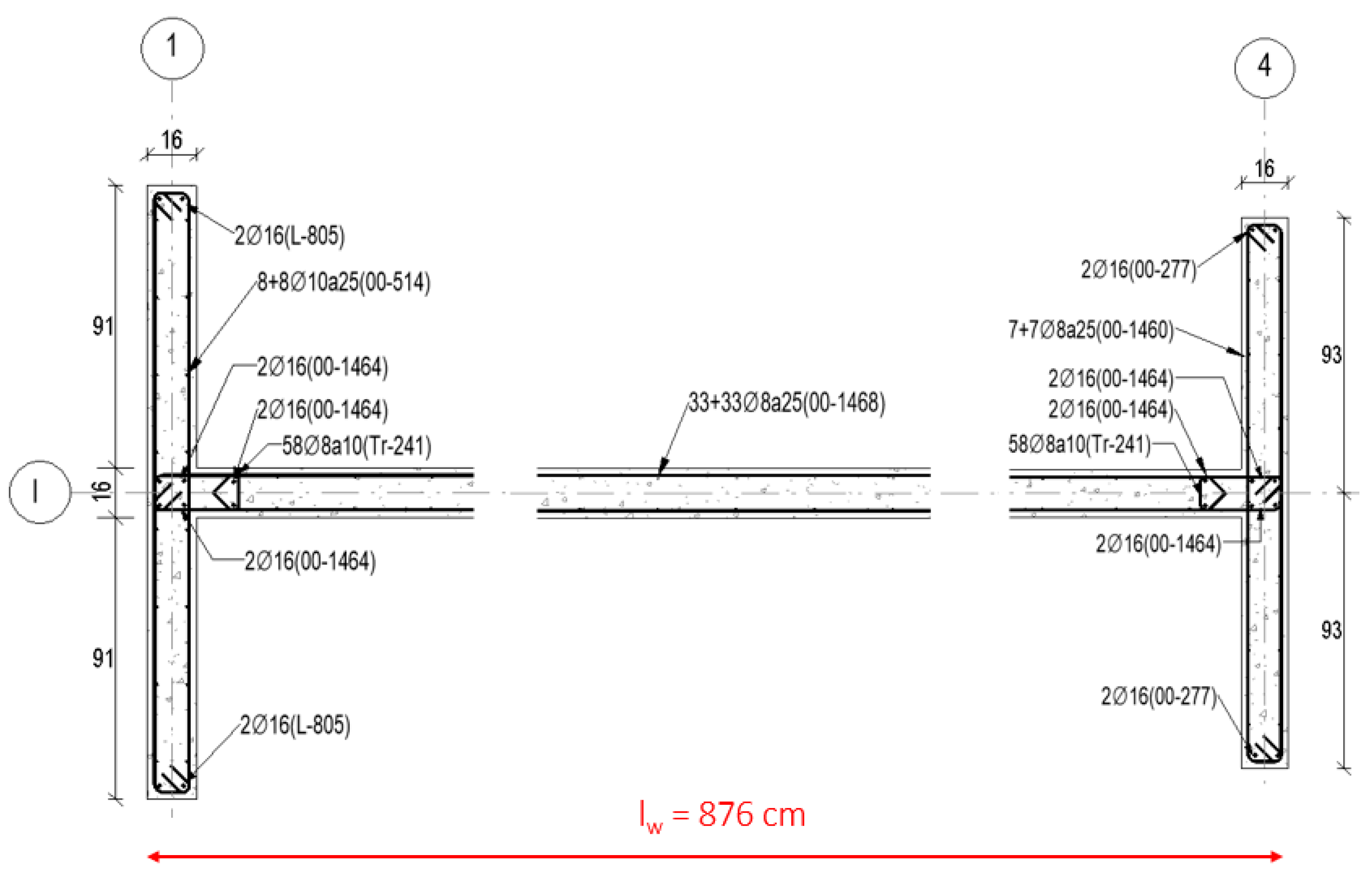Figure 2 shows an example of the reinforcement detail of one of the building’s walls.

As mentioned in Section 2.3 of this article, amendments are being proposed to the current Chilean regulations to consider the adoption of capacity design, which is not yet a mandatory requirement. However, for this study, capacity design was incorporated, using the following expression:

$$Vpr=Vu\ast {\displaystyle \frac{Mpr}{Mu}}=Vu\ast \Omega$$

(1)

$$Vpr\le \Phi Vn=0.75Vn$$

(2)

where $V_{pr}$ is the probable shear by design based on capacity, $V_u$ is the shear obtained from analysis, $V_n$ is the nominal shear of the element, $M_{pr}$ is the nominal moment of the element considering the expected material properties (Table 6), $M_u$ is the moment obtained from analysis, and $\Omega$ is the overstrength ratio. The above expressions are based on those presented in ACI 318-19 [34]. However, the dynamic shear amplification factor ($w_v$) is not considered, as the expression provided in the manual overestimates this effect in slender walls coupled by beams or slabs, which are common in Chile [39]. Consequently, it is assumed that $w_v=1$, and the capacity shear calculation is performed only considering the overstrength factor ($\Omega$), which can be significantly higher than the values suggested by ACI 318. The overstrength factor ($\Omega$) is derived from the flexural design, considering a 1.25 amplification of $f_y$ for the reinforcement, which represents the expected material strength. Under these assumptions, the values of $M_{pr}$ and $M_u$ are determined, and subsequently, the overstrength factor ($\Omega$) is calculated, taking the greater value from both principal directions.

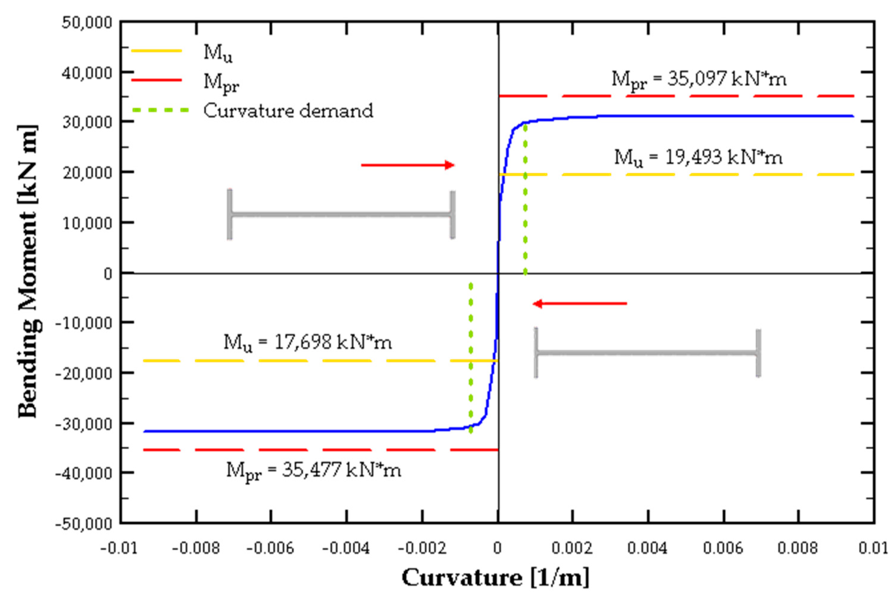
The moment–curvature curve of Wall X1 illustrates the determination of these parameters, as shown in Figure 3, where the blue line represents the nominal moment ($M_n$)–curvature relationship of the wall, obtained from section analysis; additionally, the curvature demand according to Chilean regulations [38] is also included. This demonstrates that the design is compliant with the code prescriptions, which ensures that the walls are capable of resisting the design roof displacement (${\delta }_u$) without exceeding the critical value of concrete strain (${\epsilon }_c=0.3\%$).

Subsequently, the required shear reinforcement for the walls is determined. According to the nominal shear strength calculation, this is obtained using the expressions provided in ACI 318-19 [34]:

$$V_n=A_{cv}(0.53\sqrt{f_c^{\prime }}+{\rho }_t{f}_y)$$

(3)

where $V_n$ is the nominal shear of the wall, $A_{cv}$ is the cross-sectional area of the wall, $f_c^{\prime }$ is the characteristic strength of the concrete, ${\rho }_t$ is the transverse reinforcement steel ratio, and $f_y$ is the characteristic yield strength of the steel.

From this procedure, the shear reinforcement detailing is determined, as summarized in

Table 3. Shear design example for Wall X1 considering demand and capacity design shear.

Floor	${\mathit{V}}_{\mathit{u}}$ [kN]	$\mathit{\Omega }$	${\mathit{V}}_{\mathit{p}\mathit{r}}$ [kN]	${\mathit{V}}_{\mathit{p}\mathit{r}}/\mathit{\Phi }$ [kN]	Rebar Layout	${\mathit{V}}_{\mathit{n}}$ [kN]
8	402	2	804	1072	Φ8 mm@25 cm	2797
7	696	2	1392	1856	Φ8 mm@25 cm	2797
6	961	2	1922	2563	Φ8 mm@20 cm	2797
5	1186	2	2372	3163	Φ10 mm@16 cm	5199
4	1373	2	2746	3661	Φ10 mm@16 cm	5199
3	1471	2	2942	3923	Φ10 mm@16 cm	5199
2	1451	2	2902	3869	Φ8 mm@10 cm	5297
1	1010	2	2020	2693	Φ8 mm@10 cm	5297

Note: $V_U$: Ultimate shear demand. $\Omega$: Overstrength ratio. $V_{pr}$: Capacity design shear. $V_n$: Nominal shear resistance.

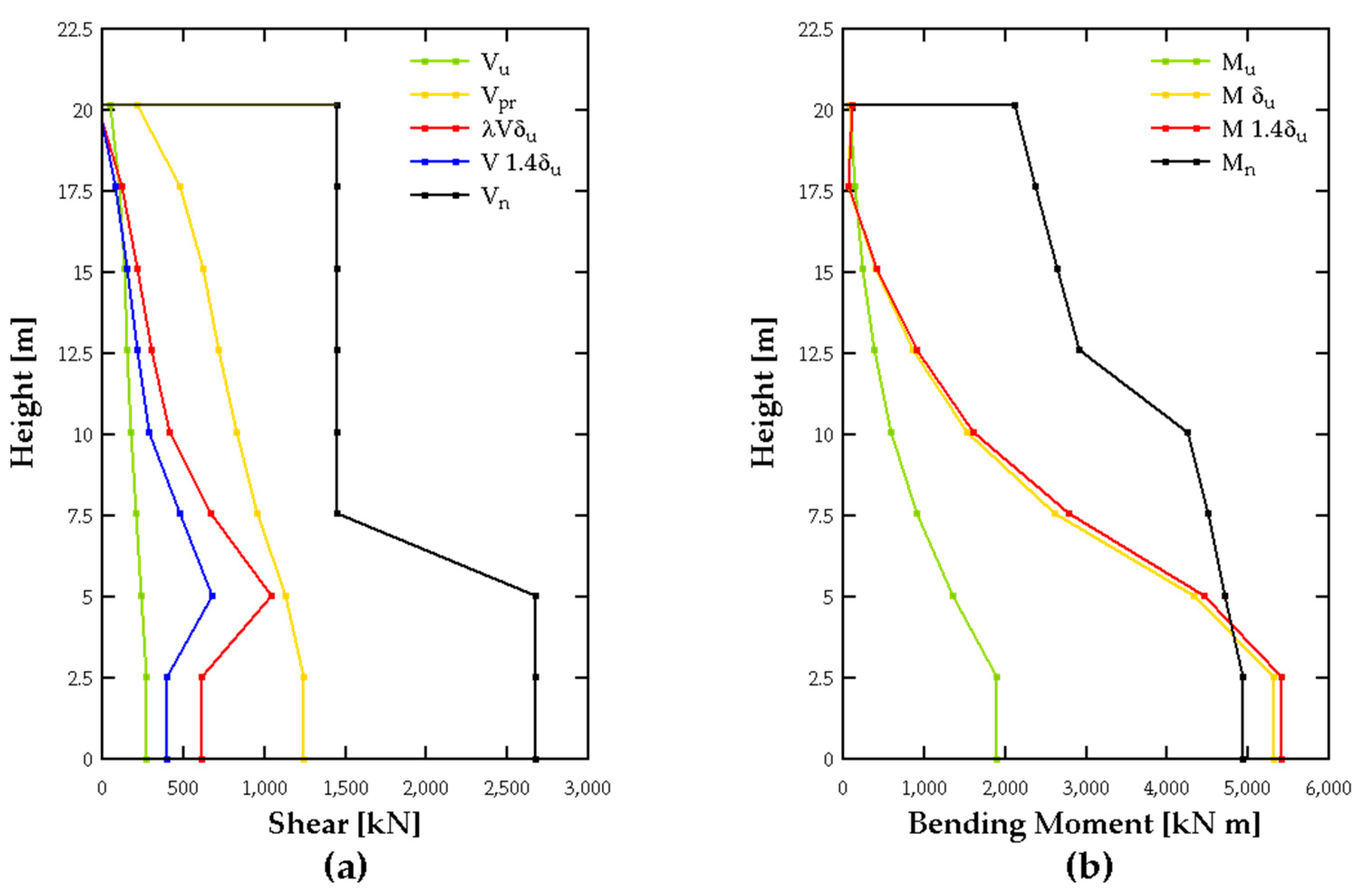
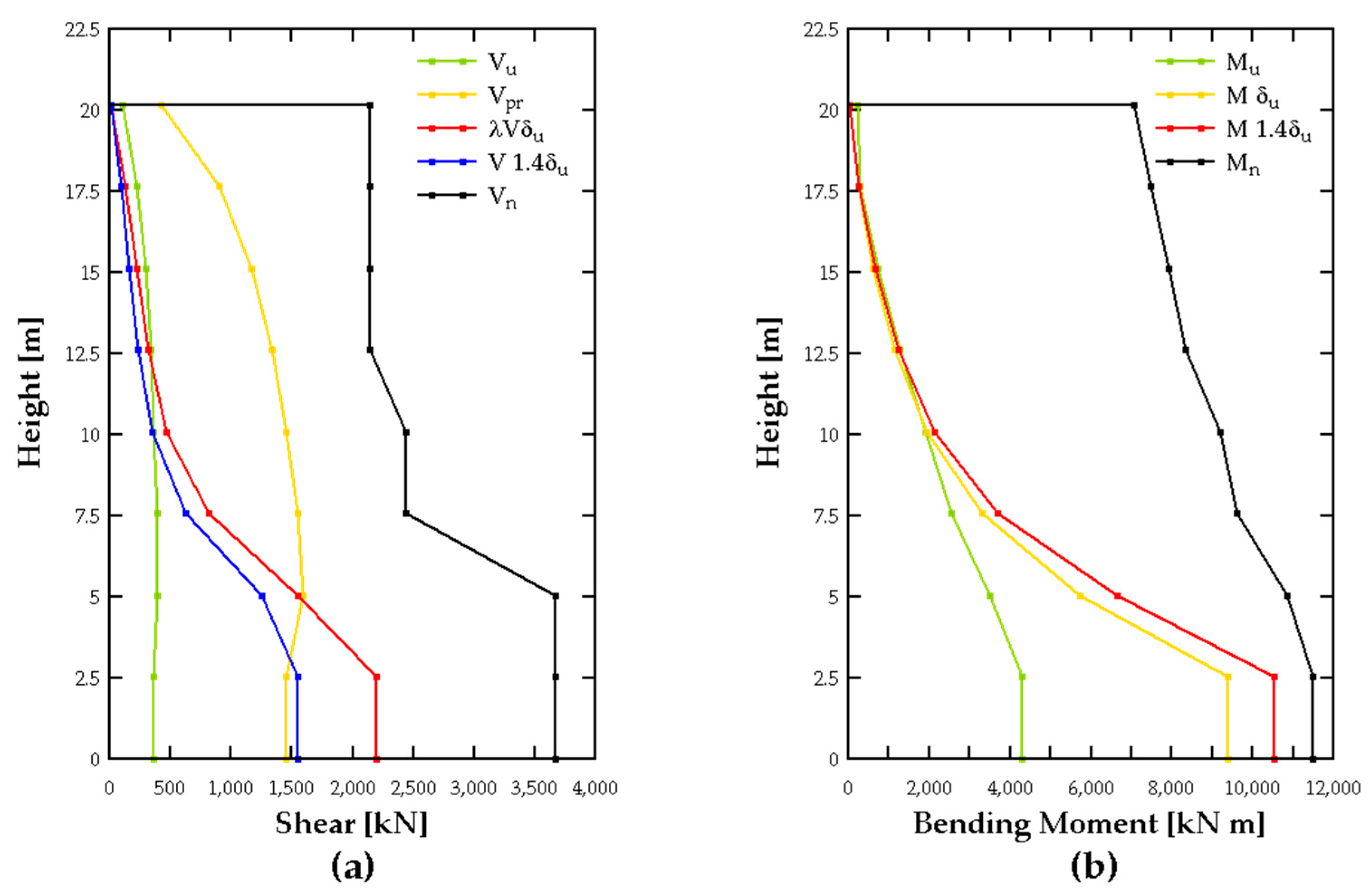
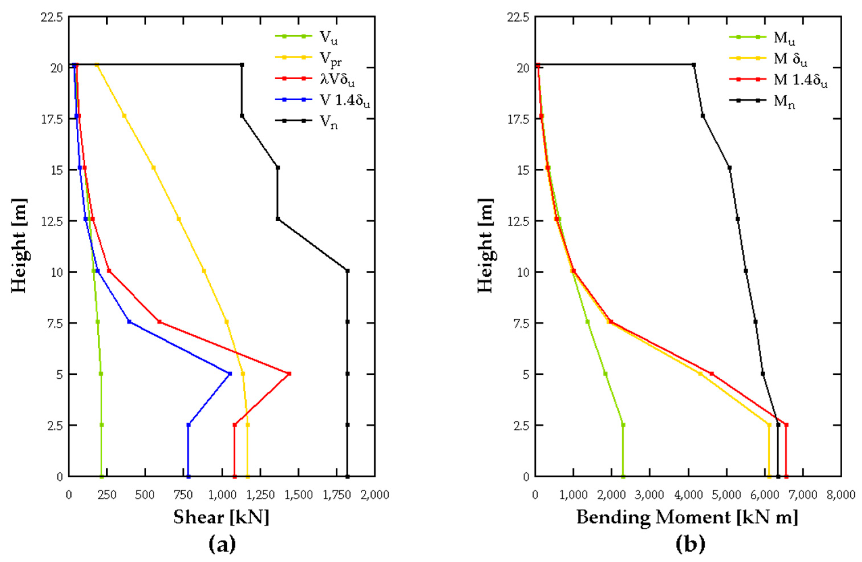
for Wall X1, which is depicted in Figure 2. Additionally, the shear force diagrams are presented in Figure 4a, comparing the ultimate shear demand, capacity shear, and nominal shear. It can be observed that the capacity shear governs the design, and that the reinforcement detailing meets the required demands.

Finally, the flexural design for the remaining floors is conducted, where the nominal moment of the wall section must be greater than the ultimate moment demand ($M_u$) and a moment envelope ($M_{env}$). The moment envelope ($M_{env}$) accounts for the effects of higher-mode contributions observed in dynamic analyses, preventing the formation of a plastic hinge outside the critical section [14].

Following practical recommendations, the moment envelope ($M_{env}$) is defined as a function of the nominal moment ($M_n$) at the critical section (first floor) and applied at half the building height (fourth floor), as described in Equation (4). For the remaining floors, a simple linear interpolation is used.

$$M_{envfloor4}=0.7M_{nfloor1}$$

(4)

The results of the flexural design, considering the ultimate moment demand ($M_u$) and the moment envelope $(M_{env}$) previously discussed, are included in

Table 4. Flexure design summary for Wall X1, considering demand and envelope moment.

Floor	${\mathit{P}}_{\mathit{u}}$ [kN]	${\mathit{M}}_{\mathit{u}}$ [kN m]	${\mathit{M}}_{\mathit{n}}$ [kN m]	${\mathit{M}}_{\mathit{e}\mathit{n}\mathit{v}}$ [kN m]	$\mathit{\Phi }{\mathit{M}}_{\mathit{n}}$ [kN m]
8	392	765	18,191	18,191	16,367
7	824	2295	20,104	19,888	18,093
6	1255	4511	23,232	21,584	20,908
5	1697	7316	25,144	23,281	22,624
4	2128	10,601	27,057	24,968	24,350
3	2569	14,180	28,998	28,537	26,095
2	3020	17,848	32,009	32,107	28,812
1	3481	20,545	35,677	35,677	32,107

Note: $P_u$: Ultimate compression demand. $M_u$: Ultimate moment demand. $M_n$: Nominal moment resistance. $M_{env}$: Moment envelope (70% of first floor $M_n$ at floor 4).

and in Figure 4b. It can be observed that the design meets the specified criteria.

3.3. Pushover Analysis Definition

Under the context of the linear design approach explained in the previous section, following both regulatory prescriptions and the inclusion of capacity design principles and higher-mode effects, the building is expected to exhibit adequate deformation capacity and ductility for the design-level seismic hazard. However, it is necessary to explicitly verify that the design meets the targeted performance objectives, which requires demonstrating compliance with the criteria specified in the ACHISINA reference manual [12].

To achieve this, the structure will be analyzed using the nonlinear static method, known as the pushover analysis, which is permitted by the reference document. This approach allows for identifying potential deficiencies that may not be apparent in the elastic design, as it considers material nonlinearities and force redistribution. The objective is to identify elements reaching critical limit states and assess the collapse mechanism of the entire structure.

For the pushover analysis, it is necessary to define an analytical model incorporating all structural elements according to their expected behavior and function. To achieve this, an analytical model was created using the commercial software ETABS (v2022) [36], using the same considerations for the definition of walls, slabs, beams, boundary conditions and diaphragm used in the linear model. However, special considerations must be taken to consider the nonlinear behavior of the structure, such as the definition of the critical section (fiber hinger) and the stiffness of the walls outside the critical section, which are explained in the following section.

The study follows the guidelines from the ACHISINA document [12], conducting the analysis in both principal directions (X and Y).

Regarding the load pattern used for the analysis, the document prescribes using a pattern corresponding to the mode with the highest translational mass. For a building with fixed-base support, this mode exhibits a triangular shape. However, for comparative purposes, an additional uniform load pattern is also considered.

The analytical model includes gravitational loads, specifically dead load (D) and live load (L), which were considered in the initial linear design. These loads are applied as an initial load state before the application of the nonlinear pushover load.

Within the dead load, non-structural elements, such as partition walls and topping slabs, are included. The live loads are considered according to their intended use, following Chilean regulations for residential apartment buildings, as detailed in

Table 5. Gravitational loads considered in the structure.

Load Type	Description	Load Value [KPa]
Live load	Departments	2
	Halls	4
	Balconies	5
Dead load	Wall partitions and slab coverings	1

.

The application of gravitational loads and the static seismic (pushover) load follows the provisions outlined in §3.5.3 [6], considering the following load condition:

$$1.0D+L_{exp}+1.0P$$

(5)

where $D$ corresponds to the dead load case, and $L_{exp}$ represents the service live load, which must be considered as 25% of the unreduced live load specified in Table 5.

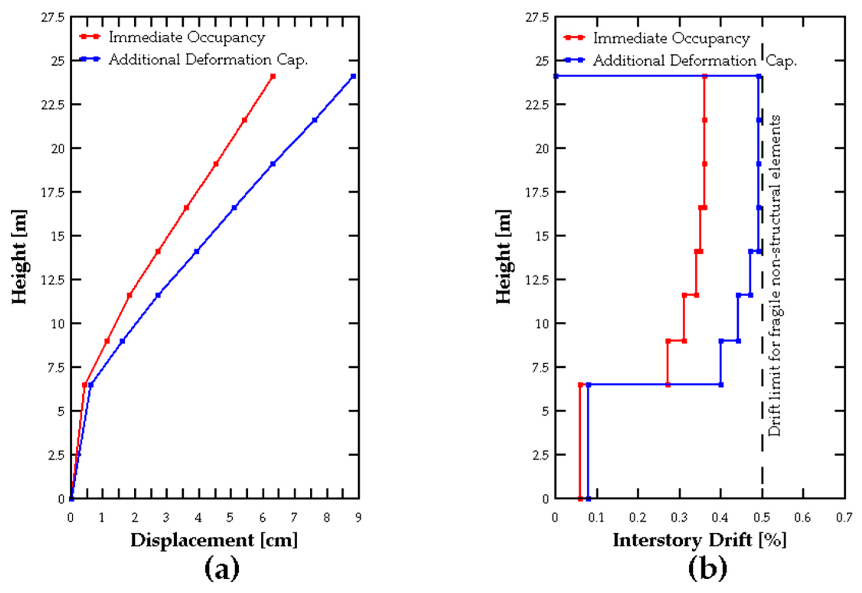
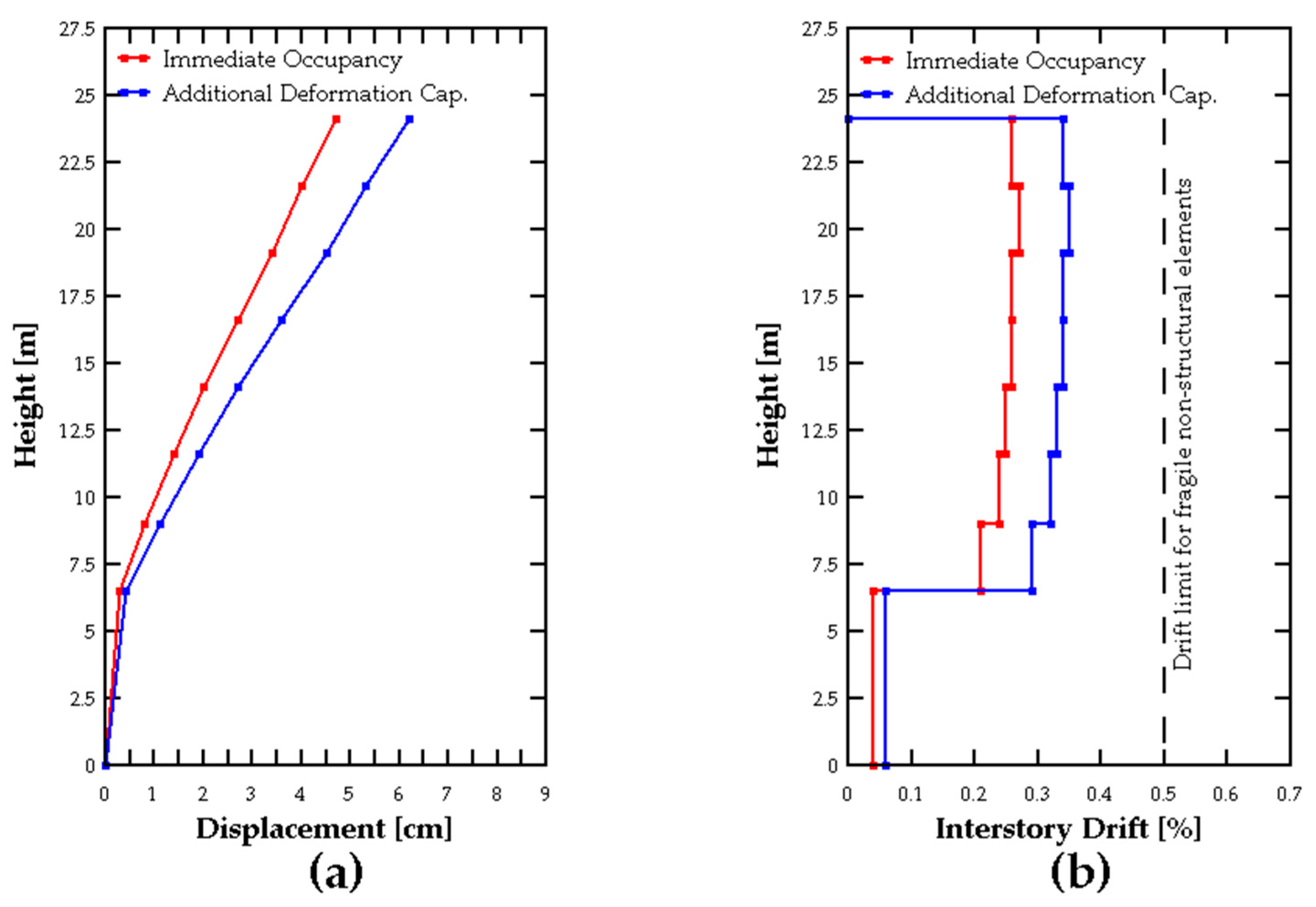
On the other hand, $P$ corresponds to the pushover load applied to the model. The reference document prescribes applying the load to achieve a roof displacement (${\delta }_u$) increased by 40% to evaluate the Additional Deformation Capacity performance objective.

For the Immediate Occupancy performance objective, a nonlinear time-history analysis (NLTHA) is recommended. However, due to the scope of this study, the evaluation is limited to analyzing the structural behavior under an equivalent condition using a pushover analysis with a roof displacement of ${\delta }_u$.

Under this context, the pushover analysis considers a target displacement of 60 cm on each direction, where the points where the roof displacement reach the values of ${\delta }_u$ and 1.4 ${\delta }_u$ in each direction are used for the compliance of the Immediate Occupancy and Additional Deformation Capacity performance objectives, respectively. The application and displacement point for the pushover analysis is on the building center of mass.

The material properties, both for linear analysis and considering overstrength as per the ACHISINA procedure [12] (according to §2.4), are summarized in

Table 6. Material characteristic and expected properties.

Material	Grade	Modulus of Elasticity (MPa)	$\mathbf{Characteristic}{\mathit{f}}_{\mathit{y}}$$/{\mathit{f}}_{\mathit{c}}^{\prime }$ (MPa)	Overstrength Ratio	$\mathbf{Expected}{\mathit{f}}_{\mathit{y}}$$/{\mathit{f}}_{\mathit{c}}^{\prime }$ (MPa)
Concrete	G25	23,500	25	1.3	32.5
Steel	A630-420H	210,000	420	1.17	491.4

.

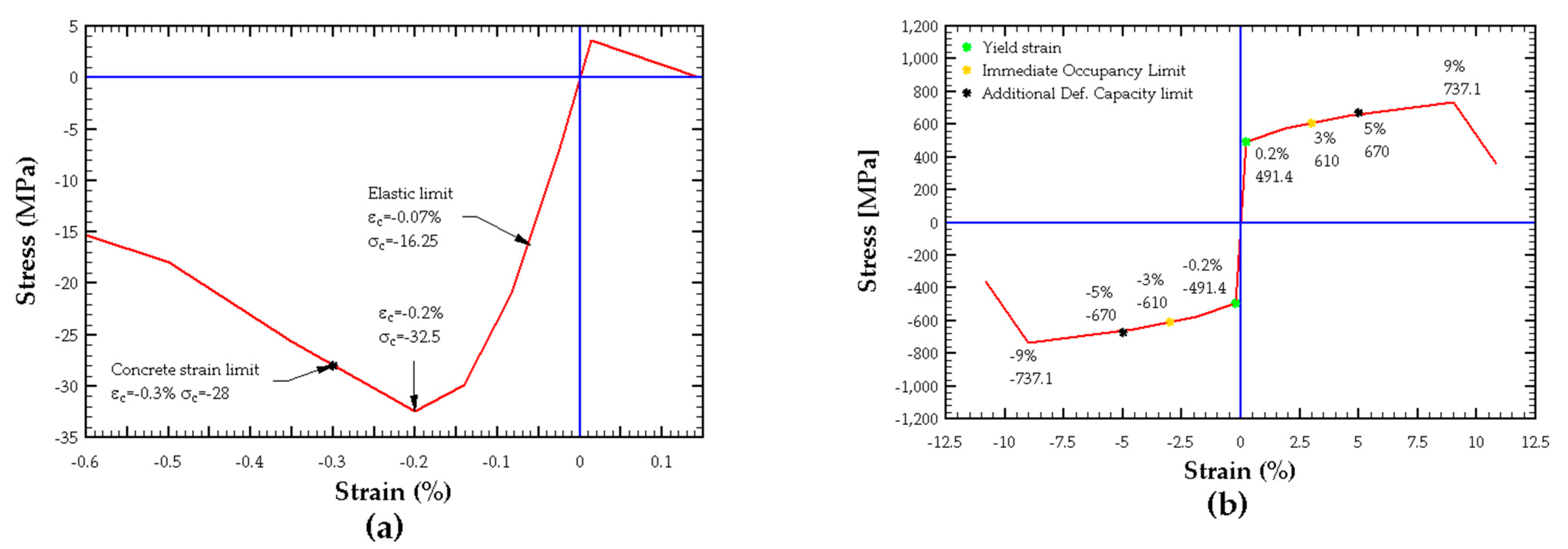
Based on these data, to represent material nonlinearity, stress–strain curves are defined for concrete and reinforcing steel. For concrete, the Mander et al. [40] curve is adopted, as shown in Figure 5a. Since special confined boundary elements are not included in the design, the unconfined concrete curve is used, which does not require additional parameters beyond the concrete’s intrinsic properties. The limit compressive strain for concrete (${\epsilon }_c$) is 0.3%, defined according to the ACHISINA criteria of acceptance shown in Table 7.

For reinforcing steel, a simplified parametric curve depicted in Figure 5b is employed. This curve is based on Holzer’s research [41], which defines three distinct behavioral regions:

• Elastic region.
• Strain hardening region.
• Strength degradation region.

Thus, the stress–strain curve is defined according to the properties of A630-420H steel, assuming that the expected strength is reached at its yield strain (${\epsilon }_y$), and including the strains limits for the Immediate Occupancy and Additional Deformation Capacity limit states, shown in Table 7.

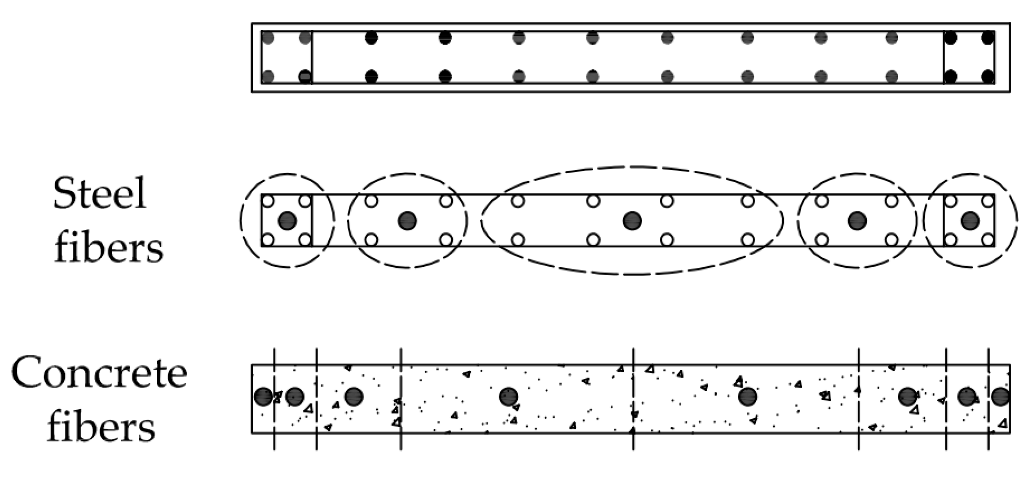
A key aspect of the analysis is the definition of the nonlinear model governing the structure. Among the various options available in the commercial software ETABS, the modeling option known as “fiber hinge” was chosen, which is a distributed plasticity model using section fibers, subsequently named in this article as a fiber section model. This model utilizes uniaxial elements (fibers) that aim to represent each material component of the cross-section, each defined by its previously established constitutive curves, as illustrated in Figure 6.

Thus, during the analysis, the element’s state is determined by integrating the response of the fibers composing its cross-section. Compared to other models, this approach offers the advantage of not requiring empirical calibration of the wall’s behavior under expected loading conditions, which is necessary for concentrated plastic hinge models. Additionally, by directly defining the stress–strain curves and integrating the fiber response, the model inherently captures the axial and flexural behavior of the element. At each analysis step, the walls with defined fiber sections update their stiffness, eliminating the need to manually modify structural stiffness to account for cracking effects. As for the walls outside the defined fiber sections, the ACHISINA manual [12] considers a stiffness modification factor of 0.5 in shear and flexure, to account for the effect of concrete cracking.

However, this model has limitations:

• It does not account for reinforcement buckling or bond-slip effects.
• It does not integrate shear forces with axial and flexural loads (P-M-V interaction).

It is important to highlight that these phenomena can be represented, but doing so would require a highly complex modeling approach, which is beyond the scope of this study. Nevertheless, fiber section models can adequately represent the response of the wall, when compared to its tested specimens under cyclic loads [42,43].

Based on the definition of the nonlinear model, it is practical to apply it only to elements expected to undergo nonlinear behavior. This approach simplifies the analysis by reducing computational time and improving result convergence.

Under this consideration, the structure was analyzed using different discretization schemes, including the following:

• One fiber section on the first floor.
• Two fiber sections on the first floor.
• Two fiber sections per two floors (for a total of four sections).
• These configurations are illustrated in Figure 7.

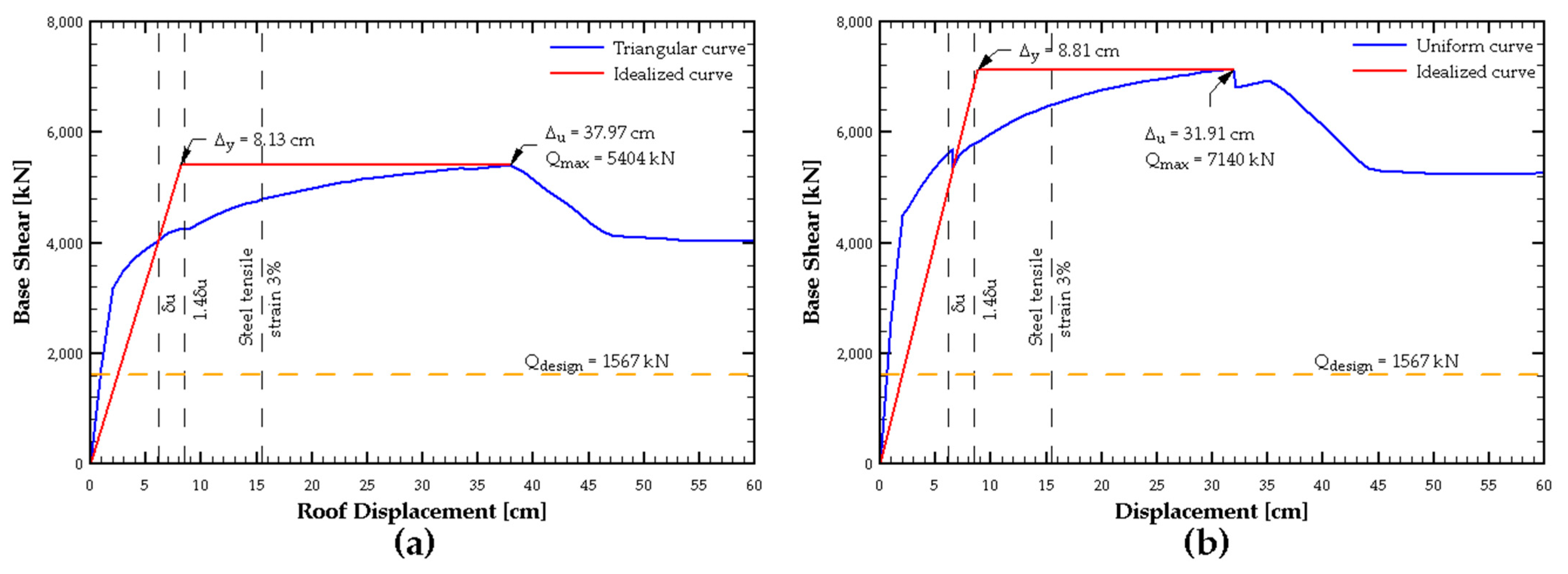
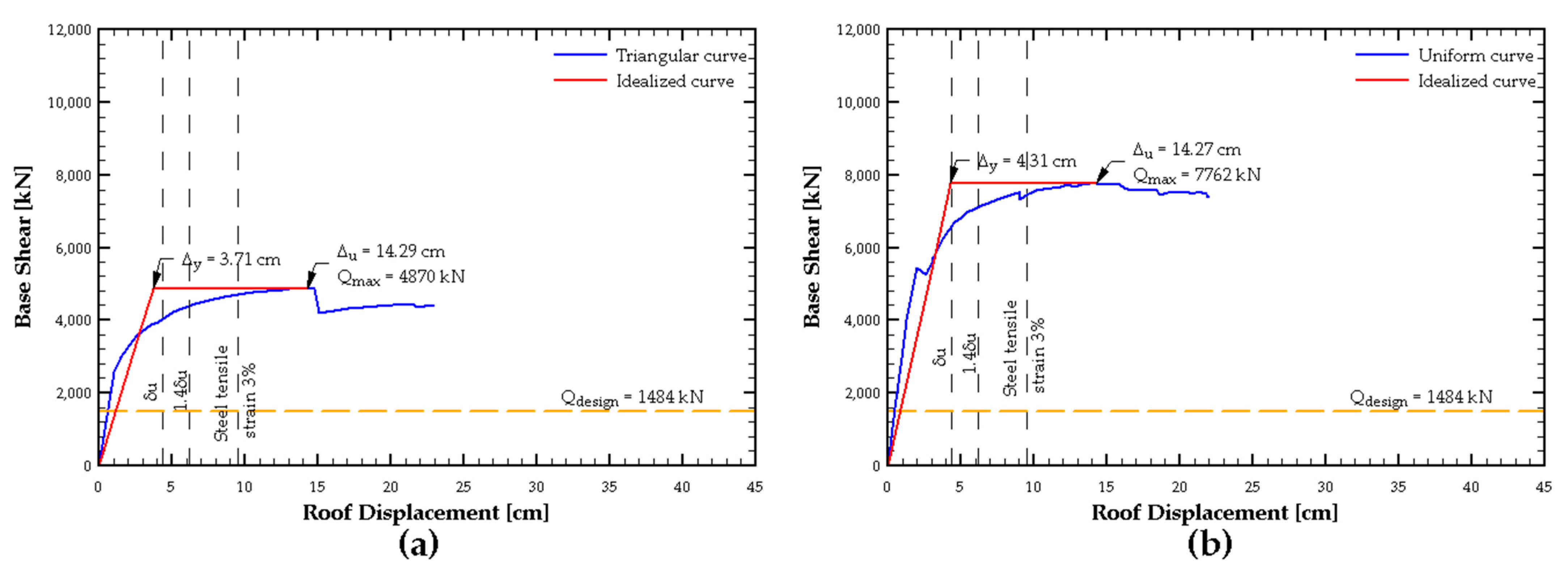
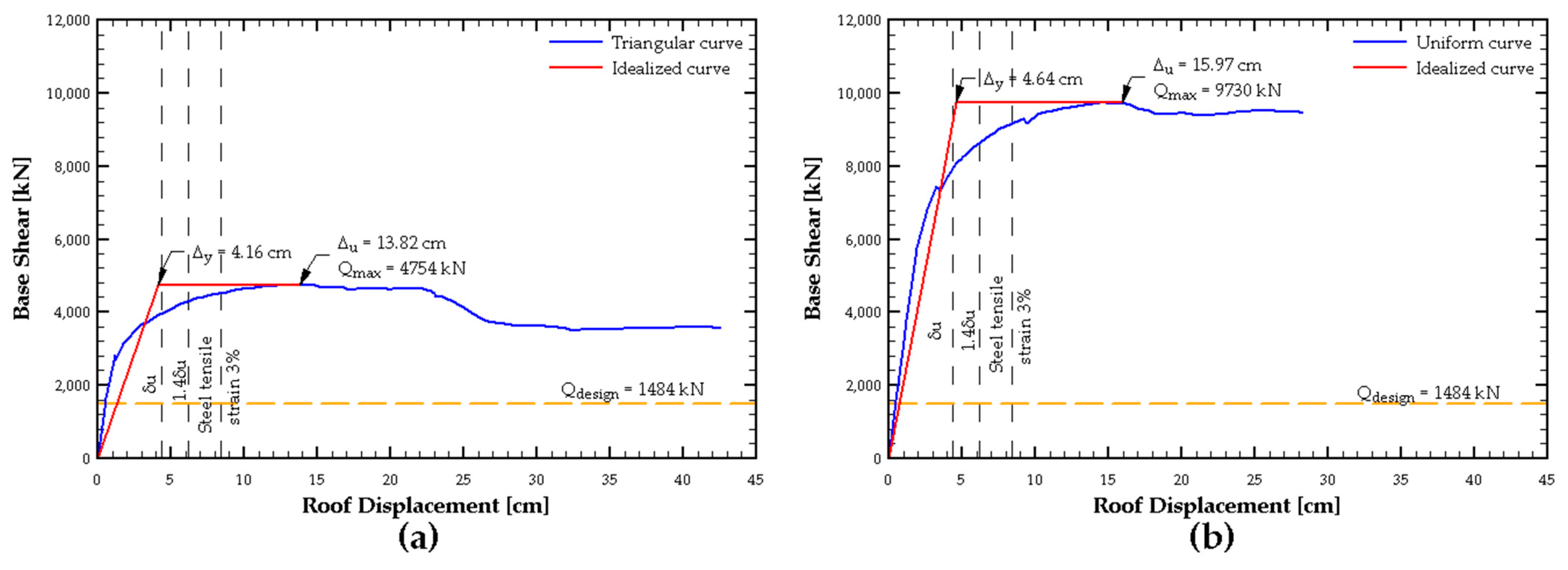
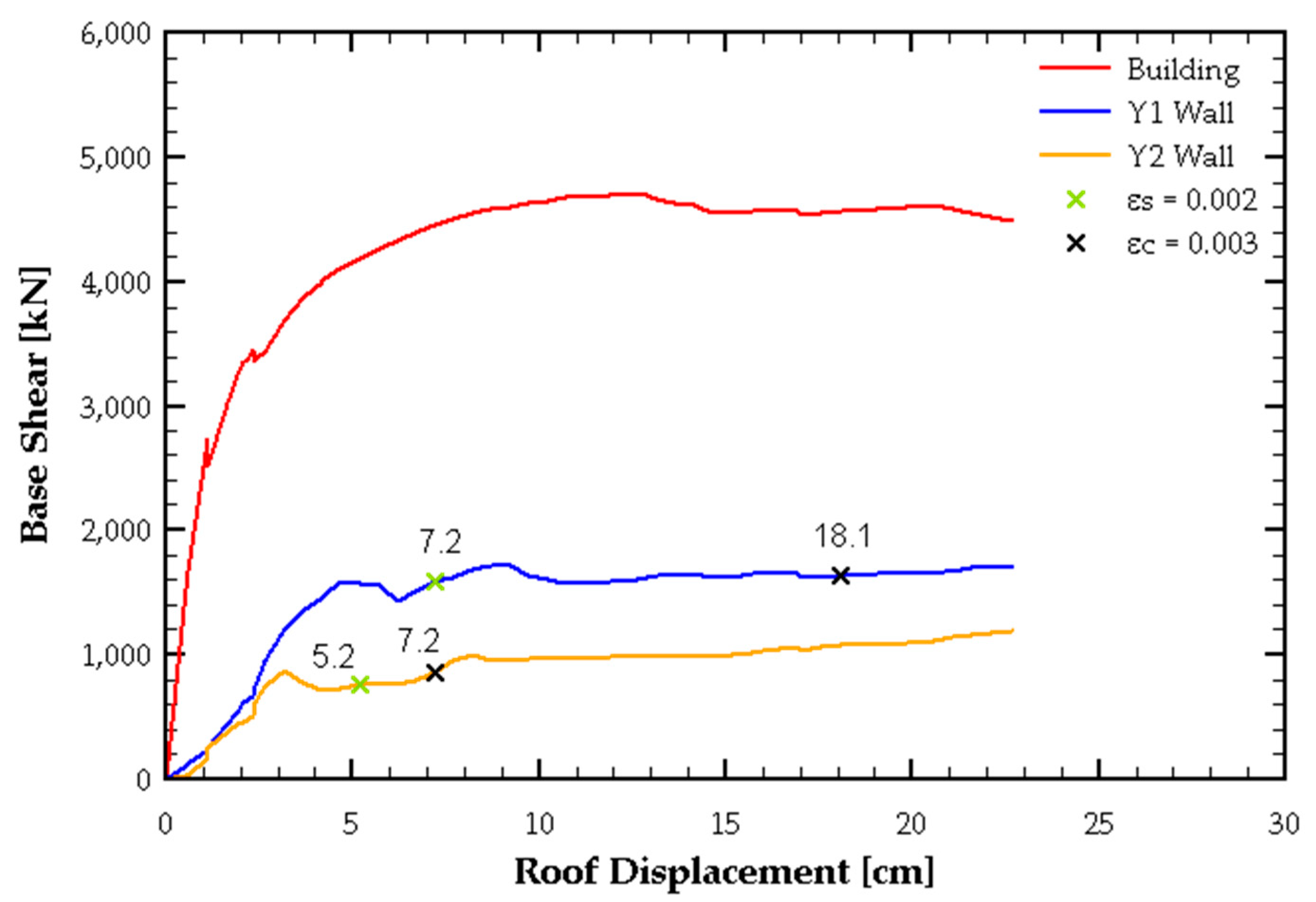
Based on this analysis, the sensitivity of the model to different discretizations was evaluated by performing a pushover analysis in the +X direction, considering both a triangular and uniform load pattern. This allowed for the capacity curve to be obtained for each case, as shown in Figure 8.

It can be observed that in the single-section model, the results converge well; however, this model does not accurately capture the degradation of the structure’s load-carrying capacity at large deformations. In contrast, the two-section model successfully represents this degradation.

On the other hand, in the four-section model, the uniform load pattern produces a behavior similar to the two-section model. However, in general, this discretization presents convergence issues, which become evident when using the triangular load pattern.

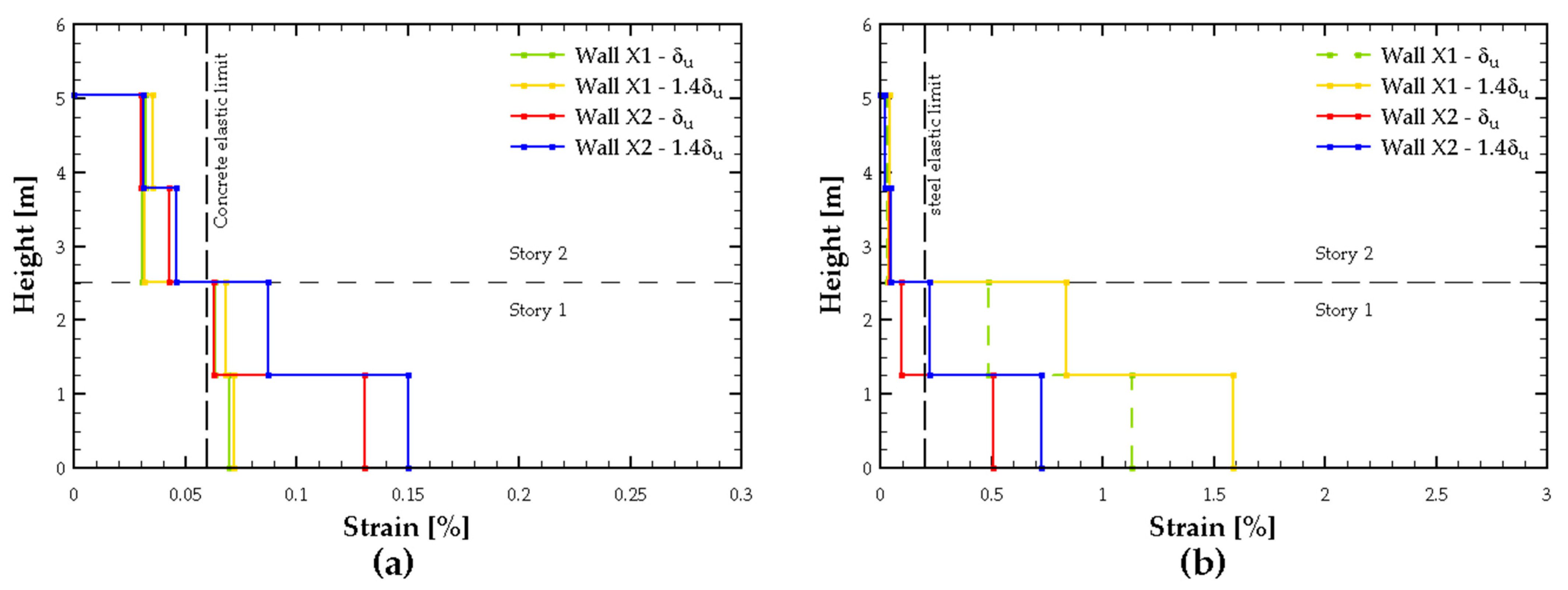
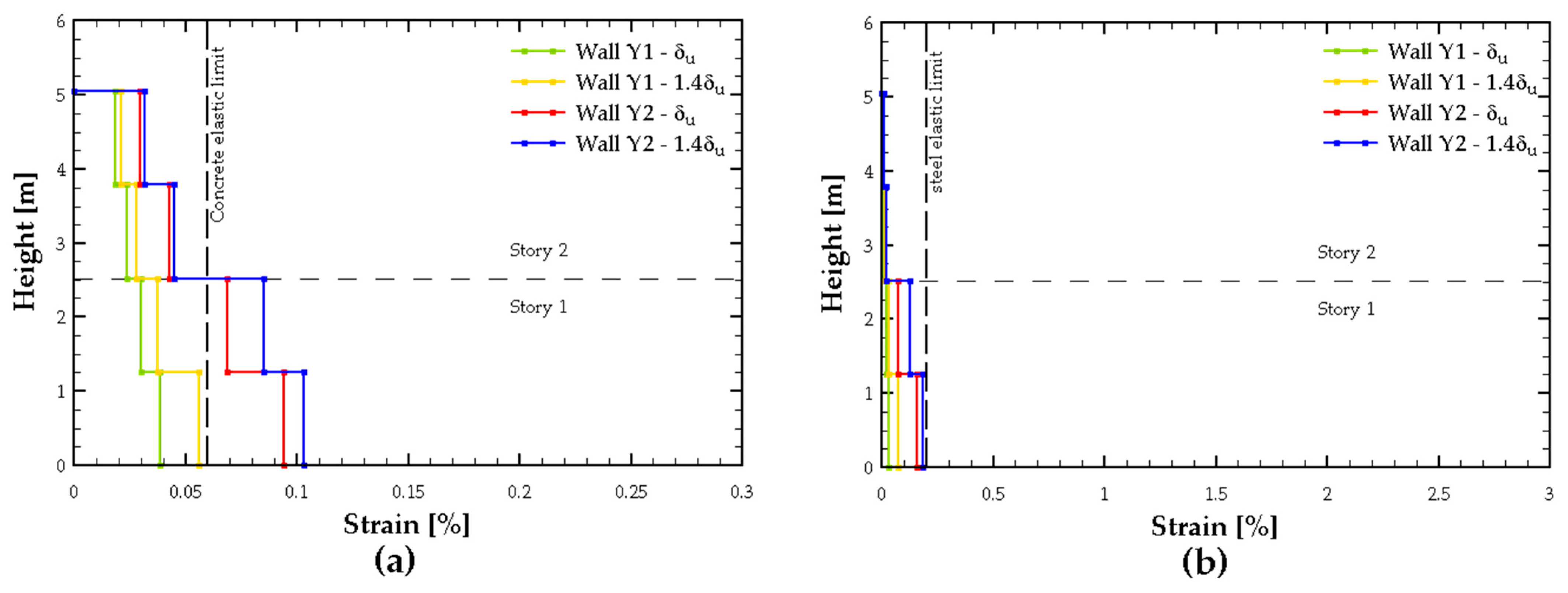
Therefore, for the next phase of this study, the two-section model located on the first floor was chosen as the primary discretization. However, the four-section model was still used to evaluate the unit strains in the walls.

3.4. Acceptance Criteria

To evaluate the building’s performance level, the procedure outlined in the ACHISINA document [12] includes performance criteria for both limit states, verifying compliance at both the global level and for the individual structural elements.

For this case study, the primary focus is on performance criteria for deformation-controlled walls and the overall stability of the building. The permissible limits for each limit state are summarized in Table 7.

Another key aspect is the review of shear forces, to ensure that the designed walls are not governed by brittle failure modes—in other words, that the walls are strength-controlled rather than displacement-controlled.

Table 7. ACHISINA manual [12] local and global acceptance criteria.

Criteria Type	Criteria	Limit Value
		Immediate Occupancy	Additional Deformation
Local	Compression unit strain in confined concrete walls	0.8%	1.5%
	Compression unit strain in unconfined concrete walls	0.3%	0.3%
	Tension unit strain in reinforcement steel of walls	3.0%	5.0%
Global	Story drifts of buildings with fragile nonstructural elements	0.5%	No limit
	Story drifts of buildings with ductile nonstructural elements	0.7%	No limit

Table 7. ACHISINA manual [12] local and global acceptance criteria.

Criteria Type	Criteria	Limit Value
		Immediate Occupancy	Additional Deformation
Local	Compression unit strain in confined concrete walls	0.8%	1.5%
	Compression unit strain in unconfined concrete walls	0.3%	0.3%
	Tension unit strain in reinforcement steel of walls	3.0%	5.0%
Global	Story drifts of buildings with fragile nonstructural elements	0.5%	No limit
	Story drifts of buildings with ductile nonstructural elements	0.7%	No limit

For this purpose, the manual provides the following formulation, which defines the acceptance criteria for force-controlled elements, depending on the considered limit state:

$${\mathsf{\lambda }F}_u\le \mathsf{\Phi }{F}_n$$

(6)

where $F_u$ is the force demand obtained from the pushover analysis, $F_n$ is the element force nominal capacity calculated according to the design codes, and $\Phi$ corresponds to the strength reduction factor, which, for the purposes of the manual, is considered as 1.0.

On the other hand, $\lambda$ is a factor dependent on the importance of the element:

• For the Immediate Occupancy limit state, $\lambda =1.5$ for critical elements and $\lambda =1.0$ for non-critical elements.
• For the Additional Deformation Capacity limit state, $\lambda$ is set to 1.0.

Therefore, as a performance criterion, given that the structural system relies entirely on the shear walls, these elements will be checked to ensure that they do not exceed the critical strength-controlled element limit.

4. Results and Discussion

In the following section, the results of the defined pushover analyses are illustrated and discussed, as described in the methodological framework, to evaluate both the global performance of the structure and the local performance of its elements, specifically the reinforced concrete walls.

It is important to emphasize that, due to the large number of elements composing the building, illustrating each one is not practical. Therefore, the analysis is limited to the walls identified in Figure 1, which are considered the most critical walls in the study.

4.1. Global Results

It is of interest to evaluate the deformation capacity of the structure using the capacity curve obtained from the pushover analysis. To achieve this, the structure is analyzed considering both a load pattern shaped by the first mode (referred to as triangular) and a completely uniform load pattern.

Based on this, the capacity curves for both directions, load orientations, and patterns are presented in Figure 9, Figure 10, Figure 11 and Figure 12. Additionally, the displacements corresponding to the Immediate Occupancy limit state and the Additional Deformation Capacity limit state are indicated as ${\delta }_u$ and $1.4{\delta }_u$, respectively. For the X direction, ${\delta }_u$ and 1.4${\delta }_u$ values are 6.3 and 8.82 cm, respectively. As for the Y direction, they are 4.5 and 6.3 cm. Furthermore, the point at which the steel deformation limit of 3% is first reached is identified, representing the location where an element exceeds the acceptance criteria defined in Table 7 for the Immediate Occupancy performance level.

Additionally, the method proposed by Park [44] is applied to determine a yield displacement, allowing for the development of an idealized bilinear curve. The method consists of calculating the yielding displacement (${\mathsf{\Delta }}_y$), considering a reduced stiffness accounting for the concrete cracking near the end of the elastic range of the curve, by using the secant stiffness at the point when base shear is 75% of the maximum base shear ($Q_{max}$) of the capacity curve. This curve is useful for estimating the ductility and overstrength values of the structure, which are presented in

Table 8. Overstrength and ductility results for Pushover Capacity curves.

Direction	Pattern	${\mathit{Q}}_{\mathit{d}\mathit{e}\mathit{s}\mathit{i}\mathit{g}\mathit{n}}$$\left[\mathbf{k}\mathbf{N}\right]$	${\mathit{Q}}_{\mathit{m}\mathit{a}\mathit{x}}$$\left[\mathbf{k}\mathbf{N}\right]$	$\mathit{\Omega }$	${\mathsf{\Delta }}_{\mathit{y}}$$\left[\mathbf{c}\mathbf{m}\right]$	${\mathit{\Delta }}_{\mathit{u}}$$\left[\mathbf{c}\mathbf{m}\right]$	$\mathit{\mu }$	$\mathit{R}$
“+X”	Triangular	1567	4990	3.18	8.51	38.67	4.54	14.47
“+X”	Uniform	1567	6644	4.24	7.45	35.99	4.83	20.48
“−X”	Triangular	1567	5404	3.45	8.13	37.97	4.67	16.11
“−X”	Uniform	1567	7140	4.56	8.81	31.91	3.62	16.50
“+Y”	Triangular	1484	4870	3.28	3.71	14.29	3.85	12.64
“+Y”	Uniform	1484	7762	5.23	4.31	14.27	3.31	17.32
“−Y”	Triangular	1484	4754	3.20	4.16	13.82	3.32	10.64
“−Y”	Uniform	1484	9730	6.56	4.64	15.97	3.44	22.57

Note: $Q_{design}$: Design base shear from linear analysis, Table 2. $Q_{max}:$ Maximum base shear. $\Omega$: Overstrength ratio. ${\mathsf{\Delta }}_y$: Yielding roof displacement. ${\mathsf{\Delta }}_u$: Ultimate roof displacement. $\mu$: Ductility. $R:$ Inherent response reduction factor.

.

It can be observed that, for all analyzed directions, the building exhibits sufficient deformation capacity for both limit states studied, remaining below the displacement threshold at which the first element exceeds the steel acceptance criteria.

Another relevant aspect is the difference between the maximum displacement and the yield displacement obtained for each direction. A clear pattern emerges where, in the X direction, the base shear is lower in the uniform pattern, while the displacement is greater compared to the Y direction. This can be explained by the differences in stiffness between both directions, where in Table 2, it is shown that the Y direction is stiffer. Another aspect to be considered is the plan asymmetry, quantified by the maximum interstory drift (relative to the CM) also shown in Table 2, where the Y direction has a higher asymmetry compared to the X direction. In other words, the X direction demonstrates greater flexibility and ductility, which can be explained by the lower plan asymmetry and density of shear walls in that direction.

As an evaluation criterion for lateral response, the results of two key indicators are considered: displacement ductility and the global overstrength reserve of the system, both calculated for the analyzed directions.

The values summarized in Table 8 show that the structure exhibits adequate ductility, exceeding a value of 3, which is considered appropriate for the structural system used in this study. Similarly, the overstrength reserve reaches values significantly greater than unity, ensuring that the structural system possesses a lateral strength far exceeding the elastic design strength.

Studies conducted on buildings with other structural typologies have validated the response reduction factors used in design. These values are compared with the inherent response reduction factors calculated by

$$R=\mu \Omega$$

(7)

The values are summarized in the last column of Table 8. It is noteworthy that, when comparing these values with the response reduction factors used in the design, they significantly exceed them.

To give more context to the results, the response reduction factors currently used in Chile are designed to significantly reduce the elastic spectra. It should be noted that the Chilean code also limits the base shear force to meet a minimum value, which requires adjusting the response reduction factor in each direction of analysis, as was considered in Section 3.1 of this article. In practice, this is achieved through an iterative process that, within a few cycles, ensures compliance with the minimum shear force. Regarding the validation of the response reduction factor, it would be interesting to apply the FEMA [18] P695 procedure [45], which has been widely used for this purpose in various studies [46,47,48,49,50].

Regarding the interstory drift criteria, for the floor deformations corresponding to both limit states, where ${\delta }_u$ is 6.3 cm and 4.5 cm for the X and Y directions, respectively, the structure complies with the stipulated limit for buildings with brittle non-structural elements, as shown in Figure 13 and Figure 14.

It is important to emphasize that results for the Additional Deformation Capacity limit state are included, even though, strictly speaking, it is not required for verification. However, it still meets the acceptance criteria for the Immediate Occupancy limit state.

From this, it can be inferred that the structure is capable of withstanding a design-level seismic hazard, exhibiting expected non-structural damage consistent with Immediate Occupancy requirements. However, it should be noted that this is a deformation-based analysis, which does not account for damage caused by accelerations—a key parameter often used to estimate this type of damage.

4.2. Local Results

4.2.1. Bending Moment and Shear Forces Results

To evaluate the local performance of the building, i.e., the performance of individual structural elements, the unit strain obtained from the analysis must be compared to the tabulated value in the manual, as referenced previously in Table 7. However, it is also of interest to examine the wall behavior in terms of forces, primarily to

• Verify that the element is not strength-controlled in shear.
• Ensure that the plastic hinge forms in the critical section defined during the design stage, which, in this case study, corresponds to the first floor.

Considering these aspects, Figure 15, Figure 16, Figure 17 and Figure 18 illustrate the comparison between the resulting forces and the nominal capacity of the element. These figures include

• Design values from the original linear model ($V_u$ and $M_u$).
• Shear strength predicted by capacity design ($V_{pr}$).
• Immediate Occupancy ($\lambda V{\delta }_u$ and $M{\delta }_u$) and Additional Deformation Capacity ($V1.4{\delta }_u$ and $M1.4{\delta }_u$) limit states.

For Walls X1 and X2, the capacity shear design realized in Table 3 and Figure 4a, effectively predicts the maximum expected shear forces in the element, as the pushover analysis results do not exceed these values. Furthermore, the flexural design successfully ensures that the plastic hinge forms in the critical section (first floor), as it is the point where the demand $M_u$ is closest or surpassing the nominal moment of the wall section.

However, a noticeable pattern is observed in the upper floors of Wall X1, where the shear force reaches higher values, and at the third floor, the bending moment approaches its nominal strength value. This suggests that the original design, as shown in Table 4 and in Figure 4b, which considered a moment envelope, may have been insufficient.

For Walls Y1 and Y2, it can be observed that capacity design also accurately predicts the expected shear force when the wall reaches its nominal moment.

However, in both walls, the shear force $\lambda V{\delta }_u$ exceeds the predicted value in some floors. This occurs because capacity design did not account for the critical element designation specified in the ACHISINA guidelines [12].

Therefore, in a preliminary design using a linear analysis, it may be of interest to consider whether an element is critical for the structural system when applying the amplification factor $\lambda$ in the formulation.

Even though the structure global behavior and wall design meets the requirements, the nonlinear pushover analysis has its limitations when it comes to reproducing the dynamic behavior of structures. Firstly, it employs a fixed pattern of lateral load distribution that corresponds to the first mode of vibration of the analyzed structure. As the structure is pushed and reaches more advanced damage states, the components lose stiffness, and the shape of the first mode is altered. Another limitation is that this method does not account for the effects of higher vibration modes, which tend to introduce greater demands in terms of both displacements and forces (moments and story shears) in the upper levels of buildings, as demonstrated in a prior study [51,52]. Additionally, it should be considered that the nonlinear pushover analysis does not adequately capture torsional effects, which arise not only from structural irregularities but also from asymmetry in damage accumulation across elements [53]. Given the above, it is recommended to complement this type of analysis with nonlinear time-history analysis (NLTHA).

Another approach includes conducting laboratory tests on a shake table with scaled models using the two horizontal components of real accelerograms to validate the numerical results.

4.2.2. Strain Results

The unit strain analysis was conducted using the four-section model to evaluate the progression of the parameter of interest along the building height and to verify the critical section hypothesis, ensuring that nonlinear deformations are concentrated on the first floor. Figure 19 and Figure 20 present the maximum unit strain results for both steel and concrete fibers under the studied limit states.

To assess the critical section hypothesis, the strain values are compared against the elastic limits of concrete (50% $f_c^{\prime }$) and steel (0.2% tensile strain) defined in Figure 5.

For Walls X1 and X2, it can be observed that both concrete and steel fibers comply with the limits established by ACHISINA [12]. Wall X1 exhibits the highest steel unit strain of 1.6%, while Wall X2 reaches a concrete strain of 0.15%.

From the results, it is noticeable that Wall X1 presents greater deformation in the steel fibers compared to the concrete fibers. This can be explained by its complex geometry, as shown in Figure 2, which allows for a larger concrete area in the compressed zone compared to the tensioned steel zone.

For Walls Y1 and Y2, the compliance with the limit criteria is also verified, showing lower values compared to the X direction, due to the greater stiffness and reduced roof displacement in the Y direction. Specifically, Wall Y1 remains in the elastic range for the evaluated limit states, while Wall Y2 reaches yield strain, as corroborated by the bending moment curves in Figure 17b and Figure 18b.

Another key observation is that the fibers remain elastic above the second floor (2.52 m and higher), validating the initial assumption that plastic hinges concentrate at the first floor. This is a crucial aspect of the analysis, as increasing the number of elements with inelastic behavior adds degrees of freedom to the structure, making result convergence more challenging.

It is also relevant to analyze the shear force in the walls as a function of displacement, which is presented alongside the +X capacity curve in Figure 21, focusing on Walls X1 and X2. From this analysis, it can be observed that the walls first reach the yield strain of the extreme reinforcement at displacements of 2.8 cm and 4.3 cm, for Walls X1 and X2, respectively. Subsequently, they exceed the steel acceptance criteria at 15.3 cm and 23.3 cm for Wall X1 and the concrete acceptance criteria at 19.3 cm for Wall X2.

Based on these findings and the shear force results, it can be concluded that the walls are deformation-controlled, which aligns with the preliminary design expectations.

The yield displacement values of the walls can be compared with empirical equations, particularly for slender walls with slab coupling, a typical feature in Chilean practice [42]. The following expression is used:

$${\delta }_y=0.22\ast 1.4\ast {\displaystyle \frac{{\epsilon }_y}{l_w}}\ast {h_w}^2$$

(8)

where ${\epsilon }_y$ corresponds to the yield strain of steel and $l_w$ and $h_w$ represent the length and height of the wall, respectively. Based on this, the calculated values from the formulation are compared with the values obtained in Figure 21, as summarized in

Table 9. Resulting and calculated yielding displacement comparison, X direction.

Wall	${\mathit{l}}_{\mathit{w}}$ [m]	${\mathit{h}}_{\mathit{w}}$ [m]	$\mathbf{Calculated}{\mathit{\delta }}_{\mathit{y}}$ [cm]	$\mathbf{Resulting}{\mathit{\delta }}_{\mathit{y}}$	Difference
X1	8.76	20.14	2.9	2.8	1.87%
X2	4.27	20.14	7.7	4.3	78.24%

.

It can be observed that the formula accurately predicts the yield displacement for Wall X1; however, for Wall X2, a 78.24% discrepancy is noted. This difference can be explained by the combined action of both walls under the pushover analysis loads. Specifically, Wall X1 reaches yield strain at a roof displacement of 2.8 cm, after which force transfer occurs to the remaining walls, including Wall X2.

Indeed, when analyzing structural components, the load transfer effect through the diaphragm must be considered. Walls with greater stiffness tend to control the yielding of other walls and, consequently, the structural response in that direction.

On the other hand, in the Y direction, a pattern similar to the X direction is observed, as shown in Figure 22. In this case, the reinforcement reaches yield strain at roof displacements of 7.2 cm and 5.2 cm for Walls Y1 and Y2, respectively. Subsequently, the concrete acceptance criterion of 0.3% strain is reached at 18.1 cm for Wall Y1 and 7.2 cm for Wall Y2.

However, it is important to note that in this direction, the steel acceptance criteria (3% and 5%) are not reached, unlike in the X direction. This indicates that the design is controlled by concrete deformation rather than steel strain.

The yield displacement values for walls in the Y direction are compared with those calculated using Equation (6), with results summarized in

Table 10. Resulting and calculated yielding displacement comparison, Y direction.

Wall	lw [m]	hw [m]	Calculated dy [cm]	Resulting dy [cm]	Difference
Y1	6.25	20.14	4.0	7.2	44.48%
Y2	3.33	20.14	7.5	5.2	44.30%

. It can be observed that the equation does not accurately predict the yield displacement for either Wall Y1 or Y2, with discrepancies exceeding 40%.

This discrepancy may be attributed to diaphragm effects due to the torsional behavior of the building, which can be explained by the plan asymmetry in that direction as seen in Section 3.1 and Table 2. This results in a different mechanism compared to the X direction, which does not present the torsional effect due to this asymmetry, and for which is not considered in the variables formulated for Equation (8).

5. Contributions to the Code Improvements in Chile

The results of this study provide concrete evidence that can inform the ongoing discussions regarding updates to Chilean seismic design codes, particularly NCh433 (Seismic Design of Buildings) [6] and the development of NCh3792 (performance-based seismic design). First, it is observed that nonlinear analysis enables clear identification of the critical section and the plastic hinge zone, providing explicit verification of the capacity design assumptions applied. This precise localization of the yielding mechanism contrasts with traditional linear models, which do not allow for an equally clear evaluation of these fundamental aspects of structural safety.

Furthermore, the results show that, in order to achieve yielding at the critical section, the shear demand may exceed the values estimated by linear design models. This discrepancy highlights that the traditional approach may underestimate certain critical demands, reinforcing the need to incorporate nonlinear analysis—such as the relatively simple pushover method—into the structural verification process. This type of analysis also yields results that are more representative of the actual behavior of structures under high-intensity earthquakes, improving predictive capabilities regarding nonlinear seismic response.

Finally, it is worth noting that nonlinear analysis provides a more accurate representation of structural behavior under severe seismic demands, delivering more realistic estimates of both demand and expected damage. In this regard, performance-based methods—such as the one proposed in the ACHISINA manual [12]—not only offer better control over the resistant mechanism and structural damage but also enable one to achieve higher levels of structural safety compared to traditional prescriptive approaches. Additionally, by explicitly incorporating deformation-based criteria and acceptable limits for damage to structural and non-structural components, these methods enhance the ability to anticipate and mitigate collateral effects such as loss of functionality or post-earthquake habitability of the building. These findings further support the need to formalize this methodology through the standardization of NCh3792 [35], promoting its systematic adoption in the design of new structures and in the evaluation of existing buildings, especially in typologies dominated by structural walls.

6. Conclusions

This study demonstrates that performance-based seismic design (PBD) is an effective tool for assessing the seismic response of reinforced concrete shear wall buildings in Chile.

The findings highlight the importance of validating prescriptive design through advanced methods such as pushover analysis to ensure compliance with performance objectives under different levels of seismic demand.

The study confirms that applying capacity design principles effectively controls shear forces and ensures ductile structural behavior.

The results indicate that using the overstrength factor leads to a safe design, although, in some cases, it may overestimate shear demand at certain floors, suggesting the need for adjustments in future regulatory frameworks.

Although pushover analysis successfully identifies failure mechanisms and verifies plastic hinge formation at the critical section of shear walls, it does not fully capture the effects of higher-mode contributions or dynamic shear amplification.

Complementing this approach with nonlinear time-history analysis (NLTHA) is recommended to assess the interaction between modal effects and progressive stiffness degradation.

The structure exhibits ductile global behavior in both principal directions, aligning with the prescriptive requirements of Chilean seismic regulations and the ACHISINA manual [12] requirements for the Immediate Occupancy limit state.

The computed response reduction factors exceed those used in linear design, suggesting that current code (NCh433 [6]) values may be more conservative than necessary. Future developments could explore configurations with smaller sections and lower steel reinforcement ratios. However, it is necessary to compare the analyses of these cases with the results obtained by applying NLTHA, so that the response alterations not captured by the nonlinear pushover analysis do not lead to results that exceed the limits considered in the design.

This study reinforces the importance of adopting performance-based design approaches in Chile, particularly for shear wall buildings, which represent a predominant structural typology in the country. Although the case study is limited to a specific building, it should be noted that it has been designed in accordance with current standards and state-of-the-art practices. While it is not advisable to extrapolate the results of the case study, these results can serve as a reference when planning the application of the methodology, understanding its limitations more clearly, and as a point of comparison for global behavior. This is particularly important as the PBD methodology is currently undergoing a standardization process as the NCh3792.

The findings suggest the need for formalizing PBD methodologies in Chilean regulations through the standardization of the ACHISINA manual [12], facilitating its systematic application in the design of new structures and the evaluation of existing ones.

Furthermore, experimental studies are recommended to validate the numerical models used, particularly regarding the interaction between structural elements and overall seismic response.