
Application of Topology Optimization as a Tool for the Design of Bracing Systems of High-Rise Buildings


Abstract
1. Introduction
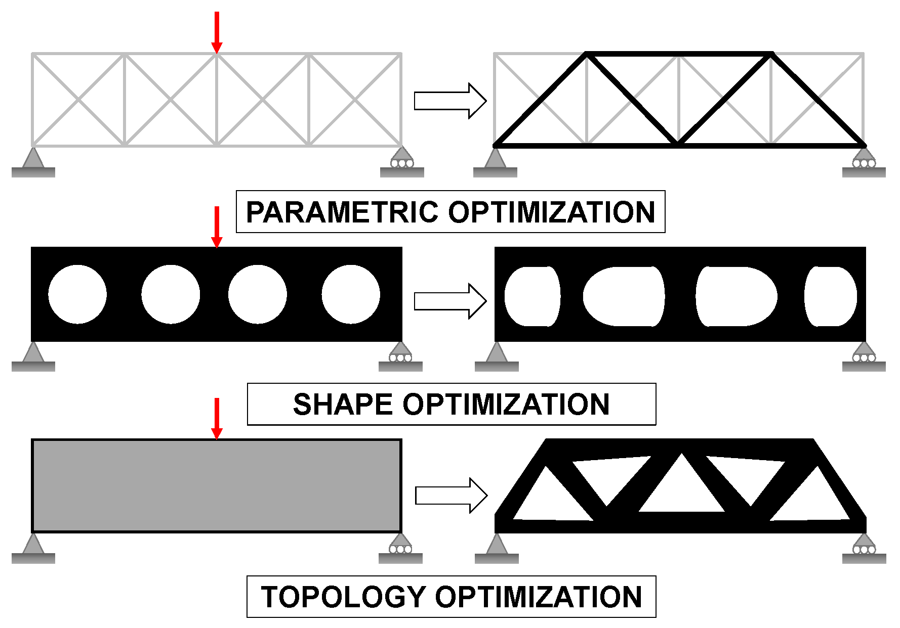
- Parametric optimization adjusts geometric variables (e.g., width, element diameter) without altering the structure’s shape or topology. The structural model remains fixed during the optimization process. In Xu et al. [10], a parametric study employed the response surface method to optimize damper parameters, simplifying the parametric analysis process and reducing computational costs.
- Shape optimization modifies the geometry to find the optimal shape within a defined domain, changing contours and hole positions without altering element connectivity.
- Topology optimization (TO) finds the optimal material distribution within a design domain, allowing changes to the connectivity of the discretized domain. Bocko et al. [11] combined topology and shape optimization, aiming to reduce weight and improve fatigue resistance, drawing inspiration from natural processes, such as trees growing.
2. Literature Survey
2.1. Wind Loads and CFD
2.2. Turbulence Modeling
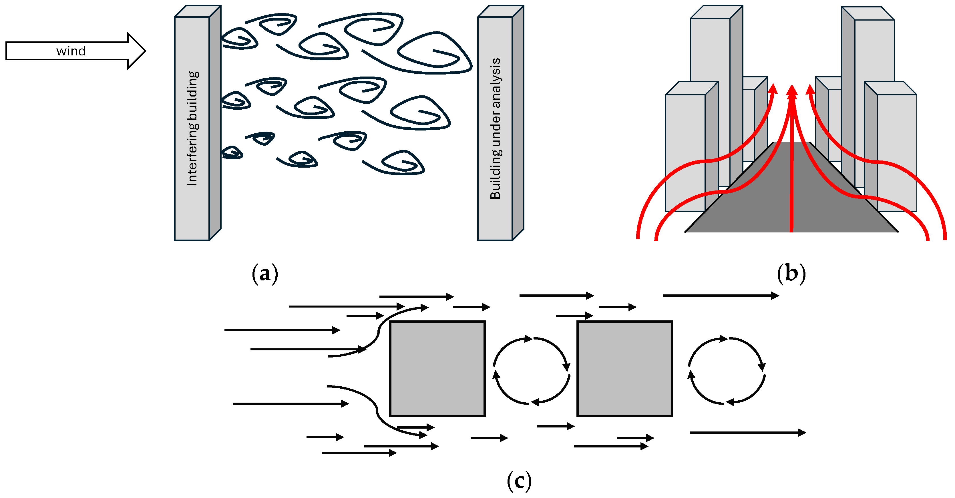
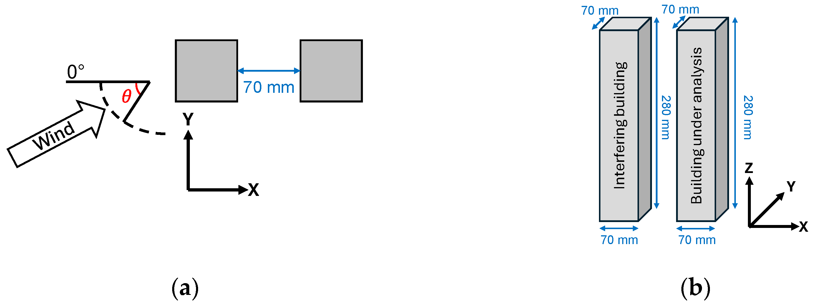
2.3. Neighborhood Effects
2.4. Structural Bracing Systems
- Rigid frames: the base elements and their connections are designed to be stiffer;
- Shear walls: adding walls to frames to increase lateral stiffness and torsional resistance;
- Outrigger: characterized by horizontal trusses or shear walls connected to the core of the structural system;
- Perforated tube systems: evenly spaced columns are connected by tall beams;
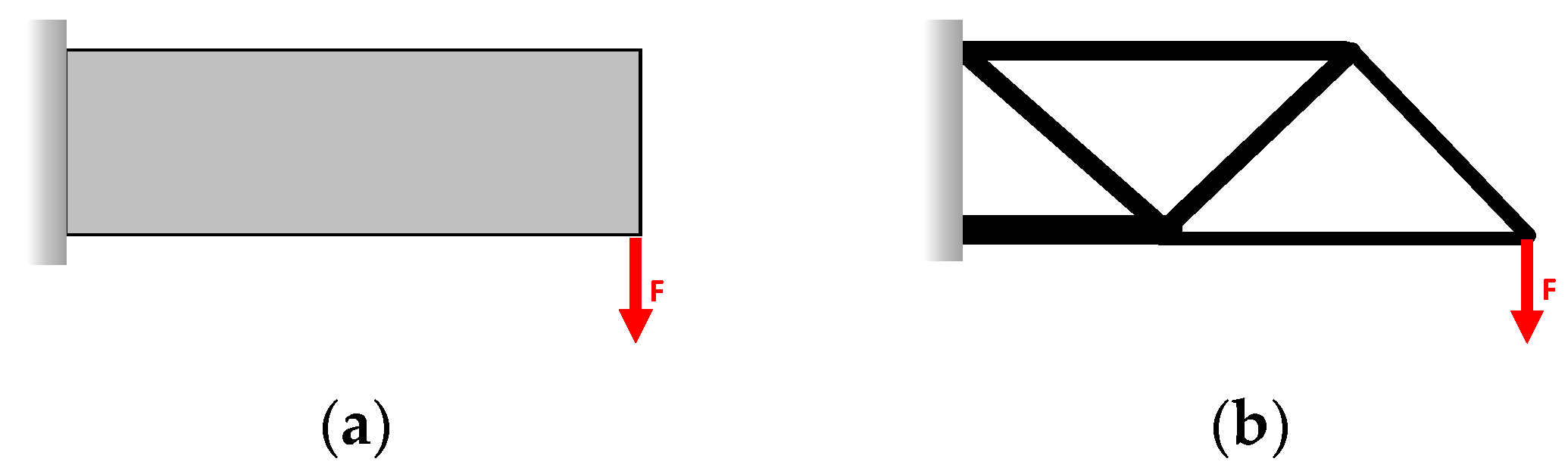
- Shear trusses: formed by placing trusses at the exterior of the structure, typically at a 45° angle;
- Tube systems: involving metal tubes arranged in irregular geometries.
2.5. Topology Optimization and BESO Method
3. Methodology
3.1. CFD Setup
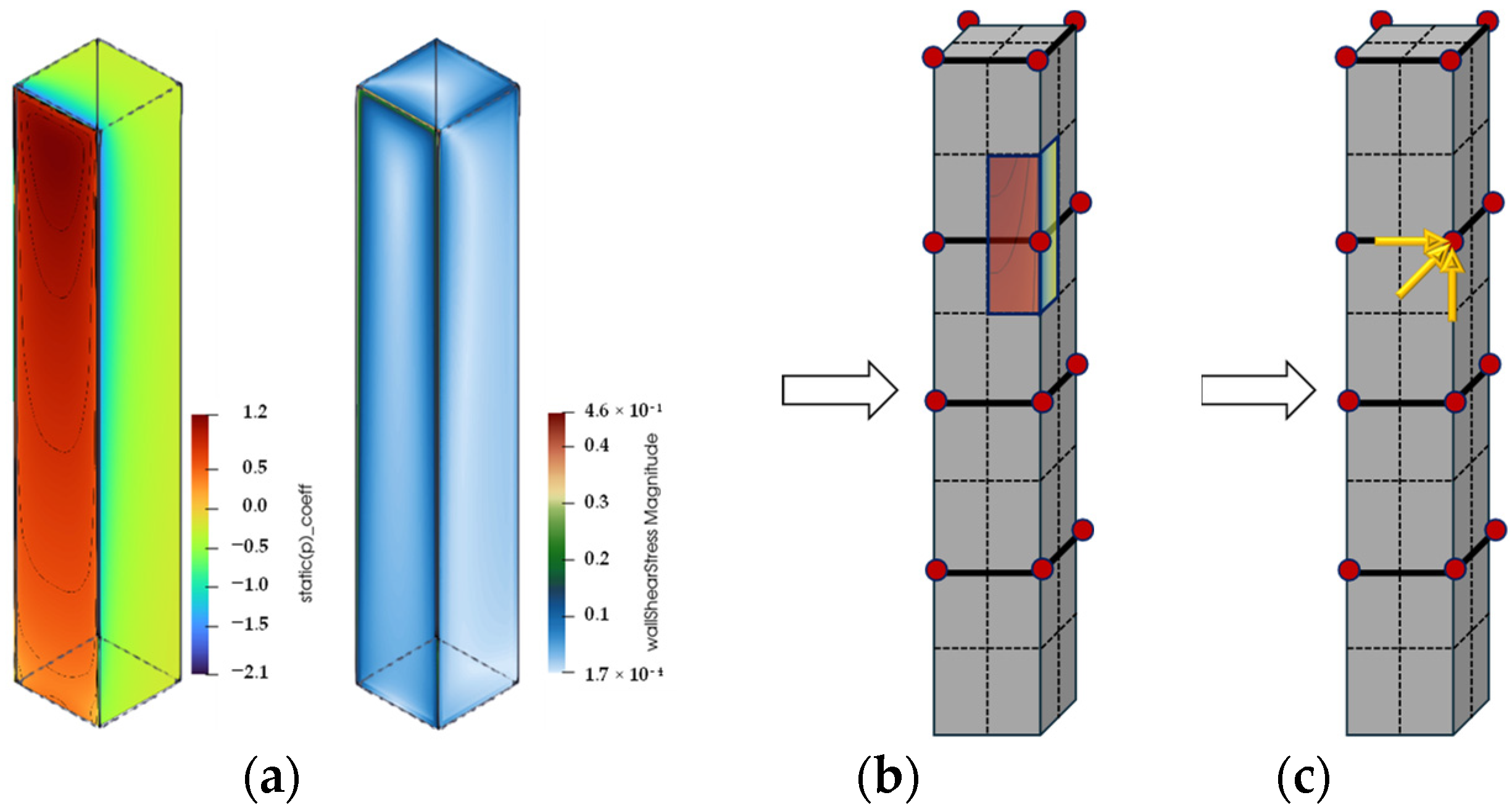
3.2. Wind Loads and Aerodynamic Coefficients
3.3. Numerical Schemes
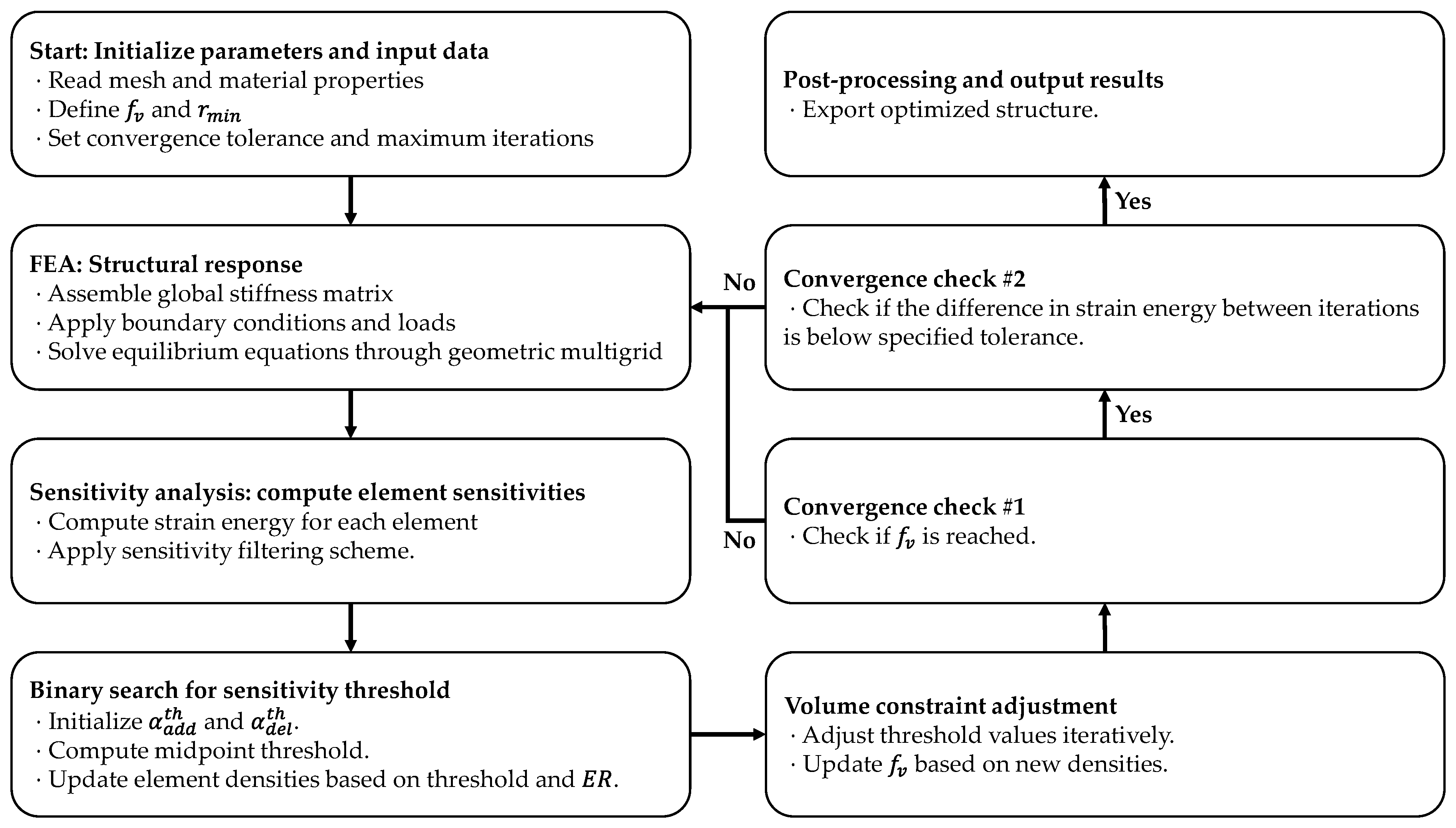
3.4. BESO Methodology for Rejection and Admission of Solid Elements
- Initialization of parameters:
- Let be the sensitivity field for the structure where each value represents the sensitivity of an individual element.
- is the design variable vector, where each value represents the material density for solid and void elements.
- and are the lower and upper bounds of the sensitivity field , respectively.
- Convergence criterion: the stopping condition is given by the relative difference between and , which must be smaller than the tolerance = 10−5.
- Binary search algorithm:
- At each iteration, the threshold is computed as follows:
- is updated based on the comparison of and , where the “sign” function returns to 1 if the argument is positive and −1 if the argument is negative.
- Volume condition: The new volume is imposed by the following condition: if the sum of the densities is greater than the volume fraction, is adjusted; otherwise, is adjusted.
- The process continues updating and until the convergence condition is met, resulting in a new vector with updated densities for the mesh elements.
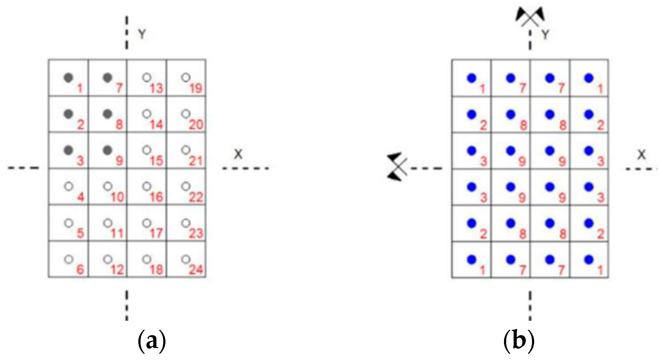
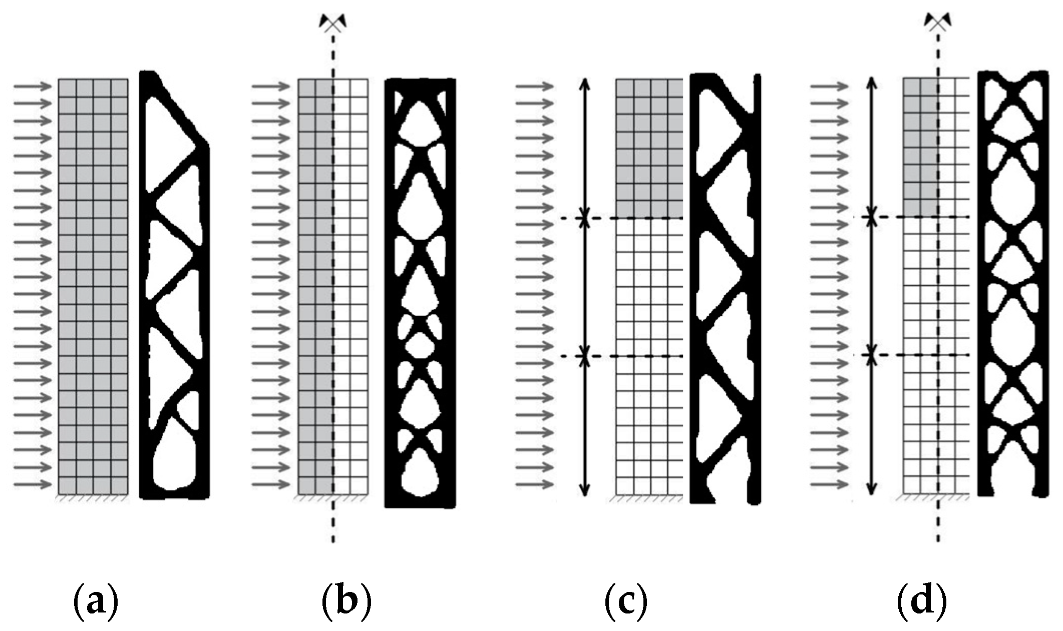
3.5. Geometric Control of BESO Results
4. Validation
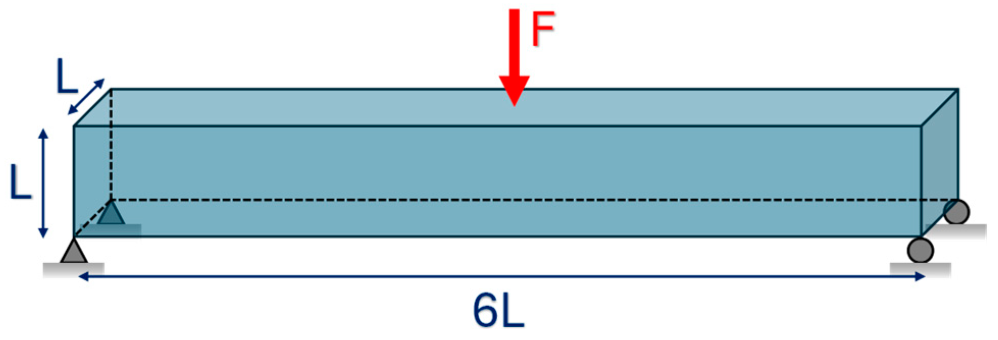
4.1. BESO Validation
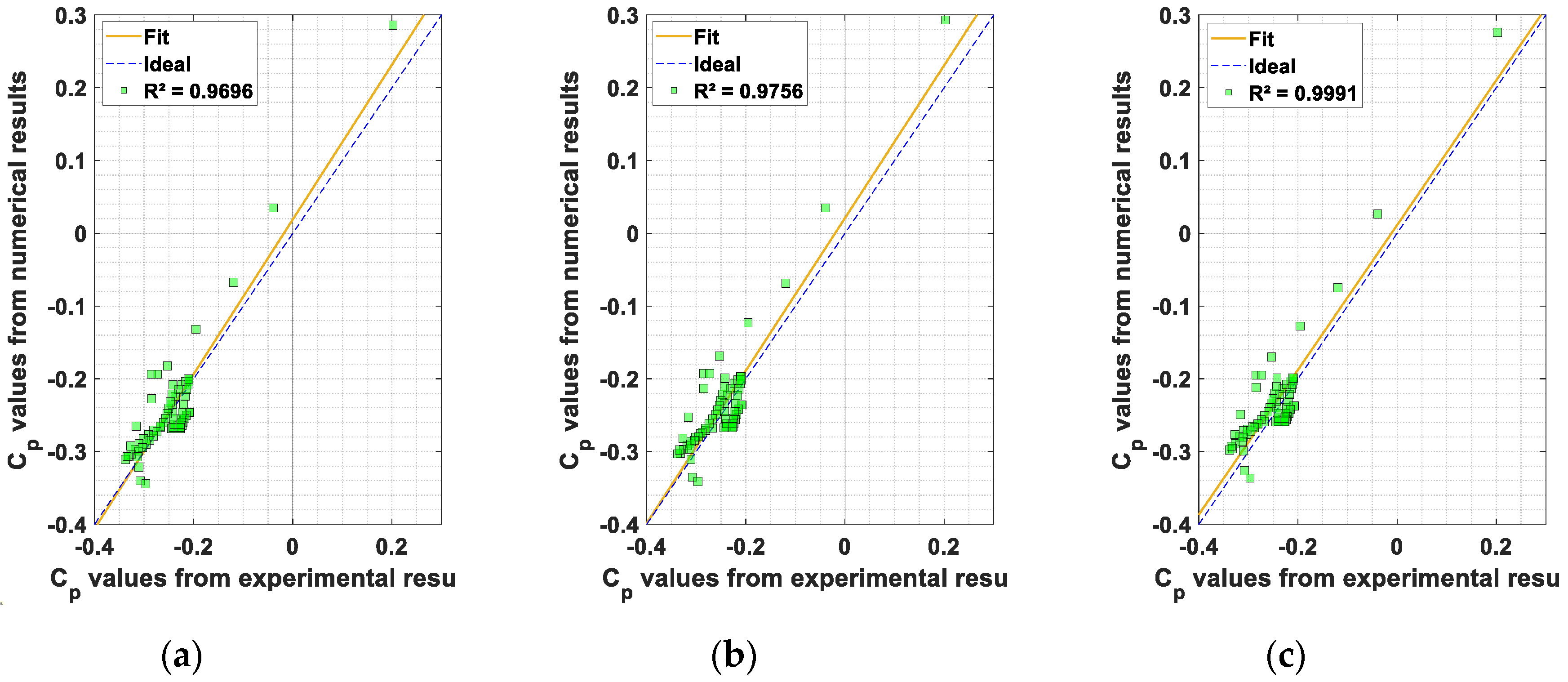
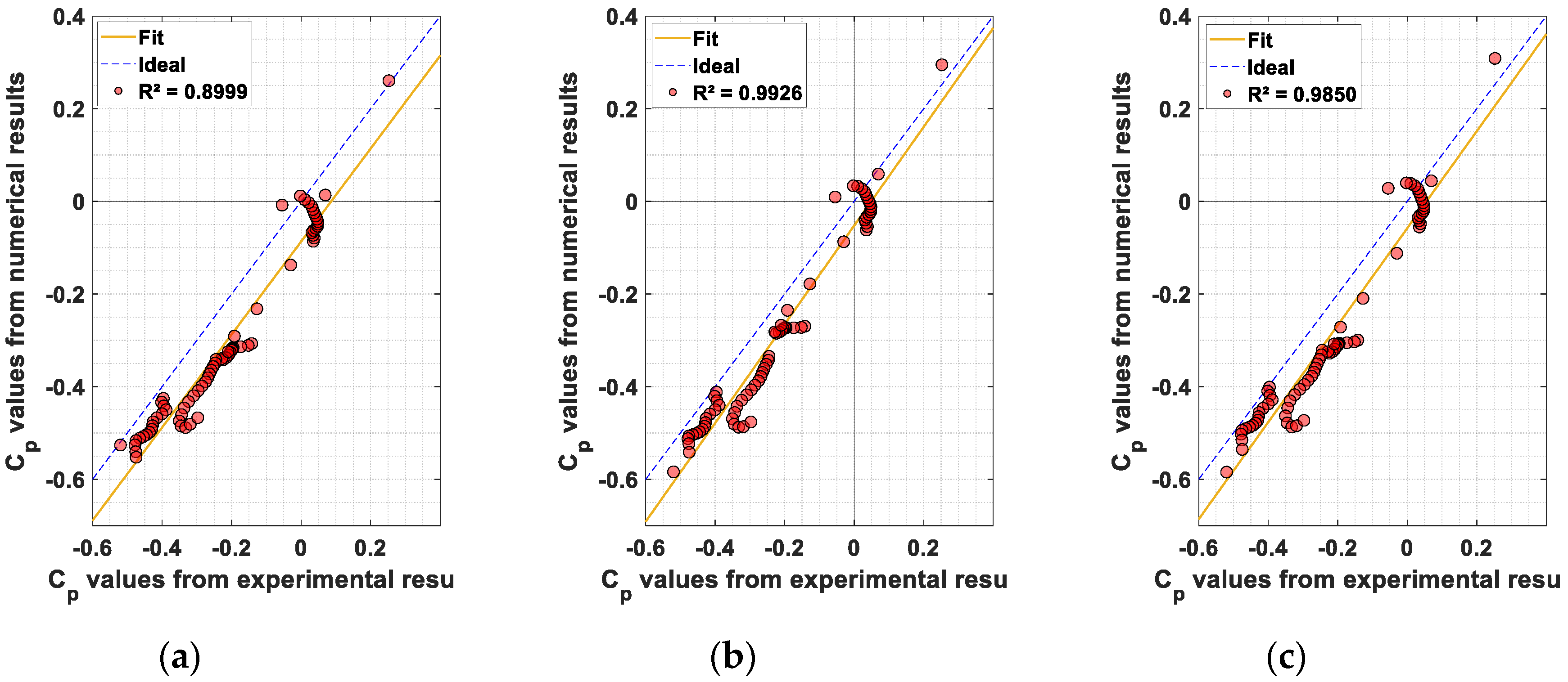
4.2. CFD Validation
5. Results
5.1. Aerodynamic Coefficients Analysis
5.2. Wind Flow and Vortices Analysis
5.3. Bracing Systems and Objective Function Analysis
5.4. Further Discussion
6. Conclusions
Author Contributions
Funding
Data Availability Statement
Conflicts of Interest
Appendix A

| Vorticity Field | Mean Pressure Coefficient Field | |
|---|---|---|
 36.73 N⋅m |  = 0.000 = 0.584 |  = 1.024 = 0.554 |
 57.00 N⋅m |  = 0.225 = 0.651 |  = 1.140 = 0.591 |
 56.76 N⋅m |  = 0.176 = 0.692 |  = 1.122 = 0.674 |
 58.55 N⋅m |  = 0.000 = 0.737 |  = 1.293 = 0.706 |
| Vorticity Field | Mean Pressure Coefficient Field | |
|---|---|---|
 37.78 N⋅m |  = 0.000 = 0.610 |  = 0.995 = 0.526 |
 53.31 N⋅m |  = 0.221 = 0.632 |  = 1.069 = 0.597 |
 54.92 N⋅m |  = 0.168 = 0.669 |  = 1.163 = 0.654 |
 53.97 N⋅m |  = 0.000 = 0.706 |  = 1.244 = 0.677 |
| Vorticity Field | Mean Pressure Coefficient Field | |
|---|---|---|
 32.99 N⋅m |  = 0.000 = 0.541 |  = 0.817 = 0.547 |
 42.33 N⋅m |  = 0.184 = 0.591 |  = 0.929 = 0.612 |
 45.80 N⋅m |  = 0.141 = 0.641 |  = 1.050 = 0.670 |
 43.24 N⋅m |  = 0.000 = 0.660 |  = 1.105 = 0.661 |
| Vorticity Field | Mean Pressure Coefficient Field | |
|---|---|---|
 20.23 N⋅m |  = 0.000 = 0.474 |  = 0.668 = 0.536 |
 29.81 N⋅m |  = 0.142 = 0.522 |  = 0.765 = 0.621 |
 36.36 N⋅m |  = 0.127 = 0.563 |  = 0.875 = 0.661 |
 33.16 N⋅m |  = 0.000 = 0.576 |  = 0.921 = 0.633 |
| Vorticity Field | Mean Pressure Coefficient Field | |
|---|---|---|
 11.06 N⋅m |  = 0.000 = 0.351 |  = 0.464 = 0.526 |
 17.95 N⋅m |  = 0.101 = 0.407 |  = 0.571 = 0.614 |
 23.94 N⋅m |  = 0.109 = 0.446 |  = 0.677 = 0.650 |
 19.98 N⋅m |  = 0.000 = 0.445 |  = 0.708 = 0.607 |
| Vorticity Field | Mean Pressure Coefficient Field | |
|---|---|---|
 3.68 N⋅m |  = 0.000 = 0.190 |  = 0.253 = 0.463 |
 8.38 N⋅m |  = 0.070 = 0.250 |  = 0.362 = 0.571 |
 11.87 N⋅m |  = 0.105 = 0.284 |  = 0.468 = 0.580 |
 9.48 N⋅m |  = 0.000 = 0.282 |  = 0.499 = 0.534 |
| Vorticity Field | Mean Pressure Coefficient Field | |
|---|---|---|
 0.29 N⋅m |  = 0.000 = 0.022 |  = 0.039 = 0.248 |
 2.41 N⋅m |  = 0.060 = 0.098 |  = 0.191 = 0.331 |
 8.30 N⋅m | 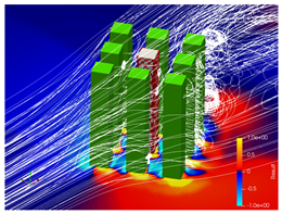 = 0.142 = 0.169 | 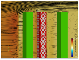 = 0.340 = 0.403 |
 5.46 N⋅m |  = 0.000 = 0.195 |  = 0.394 = 0.420 |
References
- Liu, H.; Wong, W.-K.; Cong, P.T.; Nassani, A.A.; Haffar, M.; Abu-Rumman, A. Linkage among urbanization, energy consumption, economic growth, and carbon emissions: Panel data analysis for China using ARDL model. Fuel 2023, 332, 126122. [Google Scholar] [CrossRef]
- Onat, N.C.; Kucukvar, M. Carbon footprint of construction industry: A global review and supply chain analysis. Renew. Sustain. Energy Rev. 2020, 124, 109783. [Google Scholar] [CrossRef]
- Habrah, A.; Batikha, M.; Vasdravellis, G. An analytical optimization study on the core-outrigger system for efficient design of tall buildings under static lateral loads. J. Build. Eng. 2022, 46, 103762. [Google Scholar] [CrossRef]
- Chapain, S.; Aly, A.M. Vibration attenuation in high-rise buildings to achieve system-level performance under multiple hazards. Eng. Struct. 2019, 197, 109352. [Google Scholar] [CrossRef]
- Simoncelli, M.; Tagliafierro, B.; Montuori, R. Recent development on the seismic devices for steel storage structures. Thin-Walled Struct. 2020, 155, 106827. [Google Scholar] [CrossRef]
- Jafari, M.; Alipour, A. Methodologies to mitigate wind-induced vibration of tall buildings: A state-of-the-art review. J. Build. Eng. 2021, 33, 101582. [Google Scholar] [CrossRef]
- Associação Brasileira de Normas Técnicas. NBR 6123: Forças Devidas ao Vento em Edificações; ABNT: Rio de Janeiro, Brazil, 2023. [Google Scholar]
- Shen, R.; Jiao, Z.; Parker, T.; Sun, Y.; Wang, Q. Recent application of Computational Fluid Dynamics (CFD) in process safety and loss prevention: A review. J. Loss Prev. Process Ind. 2020, 67, 104252. [Google Scholar] [CrossRef]
- Bendsøe, M.P.; Sigmund, O. Topology Optimization: Theory, Methods and Applications; Springer: Berlin/Heidelberg, Germany, 2003. [Google Scholar]
- Xu, L.; Bi, K.; Gao, J.-F.; Xu, Y.; Zhang, C. Analysis on parameter optimization of dampers of long-span double-tower cable-stayed bridges. Struct. Infrastruct. Eng. 2019, 16, 1286–1301. [Google Scholar] [CrossRef]
- Bocko, J.; Delyová, I.; Kostka, J.; Sivák, P.; Fiľo, M. Shape optimization of structures by biological growth method. Appl. Sci. 2024, 14, 6245. [Google Scholar] [CrossRef]
- Loos, S.; van der Wolk, S.; de Graaf, N.; Hekkert, P.; Wu, J. Towards intentional aesthetics within topology optimization by applying the principle of unity-in-variety. Struct. Multidisc. Optim. 2022, 65, 185. [Google Scholar] [CrossRef]
- Yang, J.-S.; Chen, J.-B.; Beer, M.; Jensen, H. An efficient approach for dynamic-reliability-based topology optimization of braced frame structures with probability density evolution method. Adv. Eng. Softw. 2022, 173, 103196. [Google Scholar] [CrossRef]
- Silva, P.U.; Pereira, R.E.L.; Bono, G. Topology optimization of bracing systems in buildings considering the effects of the wind. Struct. Eng. Mech. 2023, 86, 473–486. [Google Scholar] [CrossRef]
- Xie, L.; Yang, Z.; Xue, S.; Gong, L.; Tang, H. Topology optimization analysis of a frame-core tube structure using a cable-bracing-self-balanced inerter system. J. Build. Eng. 2024, 95, 110210. [Google Scholar] [CrossRef]
- Acosta, J.; Bojórquez, E.; Bojórquez, J.; Reyes-Salazar, A.; Ruiz-García, J.; Ruiz, S.E.; Iovinella, I. Seismic performance of steel buildings with eccentrically braced frame systems with different configurations. Buildings 2024, 14, 118. [Google Scholar] [CrossRef]
- Bezabeh, M.A.; Gairola, A.; Bitsuamlak, G.T.; Popovski, M.; Tesfamariam, S. Structural performance of multi-story mass timber buildings under tornado-like wind field. Eng. Struct. 2018, 177, 519–539. [Google Scholar] [CrossRef]
- Blessmann, J. Ação do Vento em Telhados, 2nd ed.; Editora da UFRGS: Porto Alegre, Brasil, 2009. [Google Scholar]
- Aziz, S.S.A.; Moustafa, E.B.; Said, A.-H.S.S. Experimental investigation of the flow, noise, and vibration effect on the construction and design of low-speed wind tunnel structure. Machines 2023, 11, 360. [Google Scholar] [CrossRef]
- Ljungskog, E.; Sebben, S.; Broniewicz, A. Inclusion of the physical wind tunnel in vehicle CFD simulations for improved prediction quality. J. Wind Eng. Ind. Aerodyn. 2020, 197, 104069. [Google Scholar] [CrossRef]
- You, J.-Y.; Nam, B.-H.; Park, M.-W.; You, K.-P. Comparison for assessment of wind environment in high-rise buildings using wind tunnel test and computational fluid dynamics. J. Archit. Inst. Korea 2021, 37, 163–171. [Google Scholar] [CrossRef]
- Mirzaei, P.A. CFD modeling of micro and urban climates: Problems to be solved in the new decade. Sustain. Cities Soc. 2021, 69, 102839. [Google Scholar] [CrossRef]
- Schneiderbauer, S.; Krieger, M. What do the Navier–Stokes equations mean? Eur. J. Phys. 2014, 35, 015020. [Google Scholar] [CrossRef]
- Hanjalić, K.; Launder, B. A Reynolds stress model of turbulence and its application to thin shear flows. J. Fluid Mech. 1972, 52, 609–638. [Google Scholar] [CrossRef]
- Wilcox, D.C. Formulation of the k-ω turbulence model revisited. AIAA J. 2008, 46, 2823–2838. [Google Scholar] [CrossRef]
- Ishihara, T.; Qian, G.-W.; Qi, Y.-H. Numerical study of turbulent flow fields in urban areas using modified k–ε model and large eddy simulation. J. Wind Eng. Ind. Aerodyn. 2020, 206, 104333. [Google Scholar] [CrossRef]
- Xiong, M.; Chen, B.; Zhang, H.; Qian, Y. Study on accuracy of CFD simulations of wind environment around high-rise buildings: A comparative study of k-ε turbulence models based on polyhedral meshes and wind tunnel experiments. Appl. Sci. 2022, 12, 7105. [Google Scholar] [CrossRef]
- Schalau, S.; Habib, A.; Michel, S. A modified k-ε turbulence model for heavy gas dispersion in built-up environment. Atmosphere 2023, 14, 161. [Google Scholar] [CrossRef]
- Liu, Y.; Xu, Y.; Zhang, F.; Shu, W. A preliminary study on the influence of Beijing urban spatial morphology on near-surface wind speed. Urban Clim. 2020, 34, 100703. [Google Scholar] [CrossRef]
- Blessmann, J. Introdução ao Estudo das Ações Dinâmicas do Vento, 2nd ed.; Editora da UFRGS: Porto Alegre, Brasil, 2005. [Google Scholar]
- Tomei, V.; Imbimbo, M.; Mele, E. Optimization of structural patterns for tall buildings: The case of diagrid. Eng. Struct. 2018, 171, 280–297. [Google Scholar] [CrossRef]
- Gunel, M.H.; Ilgin, H.E. A proposal for the classification of structural systems of tall buildings. Build. Environ. 2007, 42, 2667–2675. [Google Scholar] [CrossRef]
- Ali, M.M.; Moon, K.S. Advances in structural systems for tall buildings: Emerging developments for contemporary urban giants. Buildings 2018, 8, 104. [Google Scholar] [CrossRef]
- Sotiropoulos, S.; Lagaros, N.D. Optimum topological bracing design of tall steel frames subjected to dynamic loading. Comput. Struct. 2022, 259, 106705. [Google Scholar] [CrossRef]
- Resende, C.; Martha, L.F.; Lemonge, A.; Hallak, P.; Carvalho, J.; Motta, J. Automatic column grouping of 3D steel frames via multi-objective structural optimization. Buildings 2024, 14, 191. [Google Scholar] [CrossRef]
- Negarestani, M.N.; Hajikandi, H.; Fatehi-Nobarian, B.; Sardroud, J.M. Design-optimization of conventional steel structures for realization of the sustainable development objectives using metaheuristic algorithm. Buildings 2024, 14, 2028. [Google Scholar] [CrossRef]
- Gao, J.; Xiao, M.; Zhang, Y.; Gao, L. A comprehensive review of isogeometric topology optimization: Methods, applications, and prospects. Chinese J. Mech. Eng. 2020, 33, 87. [Google Scholar] [CrossRef]
- Ribeiro, T.P.; Bernardo, L.F.A.; Andrade, J.M.A. Topology Optimisation in Structural Steel Design for Additive Manufacturing. Appl. Sci. 2021, 11, 2112. [Google Scholar] [CrossRef]
- Huang, X.; Xie, Y.M. Evolutionary Topology Optimization of Continuum Structures, 1st ed.; Wiley: New Delhi, India, 2010. [Google Scholar]
- Sigmund, O.; Petersson, J. Numerical instability in topology optimization: A survey on procedures dealing with checkerboards, mesh dependencies and local minima. Struct. Multidiscip. Optim. 1998, 16, 68–75. [Google Scholar] [CrossRef]
- Lambé, A.B.; Czekanski, A. Topology optimization using a continuous density field and adaptive mesh refinement. Int. J. Numer. Methods Eng. 2017, 113, 357–373. [Google Scholar] [CrossRef]
- Bourdin, B. Filters in topology optimization. Int. J. Numer. Methods Eng. 2001, 50, 2143–2158. [Google Scholar] [CrossRef]
- Huang, X.; Xie, Y.M. Convergent and mesh independent solutions for the bi-directional evolutionary structural optimization method. Finite Elem. Anal. Des. 2007, 43, 1039–1049. [Google Scholar] [CrossRef]
- Zuo, H.Z.; Xie, Y.M. A simple and compact Python code for complex 3D topology optimization. Adv. Eng. Soft. 2015, 85, 1–11. [Google Scholar] [CrossRef]
- Franke, J.; Hirsch, C.; Jensen, A.G.; Krüs, H.W.; Schatzmann, M.; Westbury, P.S.; Miles, S.D.; Wisse, J.A.; Wright, N.G. Recommendations on the use of CFD in wind engineering. In Proceedings of the International Conference on Urban Wind Engineering and Building Aerodynamics, Sint Genesius Rode, Belgium, 5–7 May 2004. [Google Scholar]
- Tominaga, Y.; Mochida, A.; Yoshie, R.; Kataoka, H.; Nozu, T.; Yoshikawa, M.; Shirasawa, T. AIJ guidelines for practical applications of CFD to pedestrian wind environment around buildings. J. Wind Eng. Ind. Aerodyn. 2008, 96, 1749–1761. [Google Scholar] [CrossRef]
- Richards, P.J.; Hoxey, R.P. Appropriate boundary conditions for computational wind engineering models using the k-ε turbulence model. J. Wind. Eng. Ind. Aerodyn. 1993, 46–47, 145–153. [Google Scholar] [CrossRef]
- Hargreaves, D.M.; Wright, N.G. On the use of the k–ε model in commercial CFD software to model the neutral atmospheric boundary layer. J. Wind Eng. Ind. Aerod. 2007, 95, 355–369. [Google Scholar] [CrossRef]
- Launder, B.E.; Spalding, D.B. The numerical computation of turbulent flows. Comput. Methods Appl. Mech. Eng. 1974, 3, 269–289. [Google Scholar] [CrossRef]
- Martin, A.; Deierlein, G.G. Structural topology optimization of tall buildings for dynamic seismic excitation using modal decomposition. Eng. Struct. 2020, 216, 110717. [Google Scholar] [CrossRef]
- Zakian, P.; Kaveh, A. Topology optimization of shear wall structures under seismic loading. Earthq. Eng. Eng. Vib. 2020, 19, 105–116. [Google Scholar] [CrossRef]
- Zheng, X.; Montazeri, H.; Blocken, B. CFD simulations of wind flow and mean surface pressure for buildings with balconies: Comparison of RANS and LES. Build. Environ. 2020, 173, 106747. [Google Scholar] [CrossRef]
- Yadav, H.; Roy, A.K. Wind-induced aerodynamic responses of triangular high-rise buildings with varying cross-section areas. Buildings 2024, 14, 2722. [Google Scholar] [CrossRef]
- Amir, O.; Aage, N.; Lazarov, B.S. On multigrid-CG for efficient topology optimization. Struct. Multidiscip. Optim. 2014, 49, 815–829. [Google Scholar] [CrossRef]
- Zegard, T.; Paulino, G.H. Bridging topology optimization and additive manufacturing. Struct. Multidiscip. Optim. 2015, 53, 175–192. [Google Scholar] [CrossRef]
- Stromberg, L.L.; Beghini, A.; Baker, W.F.; Paulino, G.H. Topology optimization for braced frames: Combining continuum and beam/column elements. Eng. Struct. 2012, 37, 106–124. [Google Scholar] [CrossRef]
- Gholizadeh, S.; Ebadijalal, M. Performance based discrete topology optimization of steel braced frames by a new metaheuristic. Adv. Eng. Softw. 2018, 123, 77–92. [Google Scholar] [CrossRef]
- Stromberg, L.L.; Beghini, A.; Baker, W.F.; Paulino, G.H. Application of layout and topology optimization using pattern gradation for the conceptual design of buildings. Struct. Multidiscip. Optim. 2011, 43, 165–180. [Google Scholar] [CrossRef]
- Chun, J.; Song, J.; Paulino, G.H. System-reliability-based design and topology optimization of structures under constraints on first-passage probability. Struct. Saf. 2019, 76, 81–94. [Google Scholar] [CrossRef]
- Ma, J.; Lu, H.; Lee, T.-U.; Liu, Y.; Bao, D.W.; Xie, Y.M. Topology optimization of shell structures in architectural design. Archit. Intell. 2023, 2, 22. [Google Scholar] [CrossRef]
- Silva, P.U. Emprego de Otimização Topológica e DFC no Projeto de Sistemas de Contraventamento em Ambientes Urbanos. Master’s Thesis, Universidade Federal de Pernambuco, Caruaru, Brazil, 23 May 2022. Available online: https://repositorio.ufpe.br/handle/123456789/47230 (accessed on 14 March 2025).
- Liu, K.; Tovar, A. An efficient 3D topology optimization code written in Matlab. Struct. Multidiscip. Optim. 2014, 50, 1175–1196. [Google Scholar] [CrossRef]
- Sigmund, O. A 99 line topology optimization code written in Matlab. Struct. Multidiscip. Optim. 2001, 21, 120–127. [Google Scholar] [CrossRef]
- Andreassen, E.; Clausen, A.; Schevenels, M.; Lazarov, B.S.; Sigmund, O. Efficient topology optimization in MATLAB using 88 lines of code. Struct. Multidiscip. Optim. 2011, 43, 1–16. [Google Scholar] [CrossRef]
- Kosutova, K.; van Hooff, T.; Vanderwel, C.; Blocken, B.; Hensen, J. Cross-ventilation in a generic isolated building equipped with louvers: Wind-tunnel experiments and CFD simulations. Build. Environ. 2019, 154, 263–280. [Google Scholar] [CrossRef]
- Du, Y.; Blocken, B.; Abbasi, S.; Pirker, S. Efficient and high-resolution simulation of pollutant dispersion in complex urban environments by island-based recurrence CFD. Environ. Model. Softw. 2021, 145, 105172. [Google Scholar] [CrossRef]
- Qin, P.; Ricci, A.; Blocken, B. On the accuracy of idealized sources in CFD simulations of pollutant dispersion in an urban street canyon. Build. Environ. 2024, 265, 111950. [Google Scholar] [CrossRef]
- New Frontier of Education and Research in Wind Engineering Proposed by School of Architecture and Wind Engineering at the Tokyo Polytechnic University. Available online: http://www.wind.arch.t-kougei.ac.jp/system/eng/contents/code/tpu (accessed on 8 January 2025).
- Du, M.; Yan, B.; Zhou, X.; Yang, Q.; Wang, L.; Li, X.; He, Y.; Liang, Q. Interference effects of a neighboring building with various rotation angles on wind pressures of a high-rise building. J. Wind Eng. Ind. Aerodyn. 2024, 246, 105657. [Google Scholar] [CrossRef]
- Dokhaei, B.; Abdelaziz, K.; Shafei, B.; Sarkar, P.; Hobeck, J.; Alipour, A. Aeroelastic boundary layer tests of a 1:76 model of tall building and effects of adjacent building interference. J. Wind Eng. Ind. Aerodyn. 2025, 257, 106006. [Google Scholar] [CrossRef]
- Goli, A.; Alaghmandan, M.; Barazandeh, F. Parametric structural topology optimization of high-rise buildings considering wind and gravity loads. J. Architect. Eng. 2021, 27, 04021038. [Google Scholar] [CrossRef]
- Baghbanan, A.M.; Alaghmandan, M.; Golabchi, M.; Barazandeh, F. Architectural form finding and computational design of tall buildings applying topology optimization against lateral loads. J. Architect. Eng. 2023, 29, 04022038. [Google Scholar] [CrossRef]


| Mesh Resolution | BESO (MGCG) | Liu and Tovar [62] SIMP (PCG) | Amir et al. [54] SIMP (MGCG) |
|---|---|---|---|
| 60 × 10 × 10 (M1) |  C = 20.57 Time: 0.11 |  C = 28.75 Time: 1.04 |  C = 24.02 Time = 0.22 |
| 120 × 20 × 20 (M2) |  C = 11.61 Time: 1.00 |  C = 17.05 Time: 11.79 |  C = 16.49 Time: 1.52 |
| 180 × 30 × 30 (M3) |  C = 9.79 Time: 4.13 |  C = 13.49 Time: 62.67 |  C = 11.54 Time: 4.30 |
| Case | Fit Equation | R2 | FB | FAC2 | RMSE | MAE |
|---|---|---|---|---|---|---|
| 0° M1 | 1.063x + 0.019 | 0.9696 | 0.270 | 0.930 | 0.020 | 0.017 |
| 0° M2 | 1.049x + 0.021 | 0.9756 | 0.274 | 0.930 | 0.021 | 0.018 |
| 0° M3 | 0.995x + 0.011 | 0.9991 | 0.145 | 0.954 | 0.012 | 0.012 |
| 15° M1 | 1.003x − 0.087 | 0.8999 | 0.429 | 0.837 | 0.087 | 0.087 |
| 15° M2 | 1.065x − 0.052 | 0.9926 | 0.246 | 0.913 | 0.057 | 0.052 |
| 15° M3 | 1.047x − 0.058 | 0.9850 | 0.219 | 0.911 | 0.060 | 0.058 |
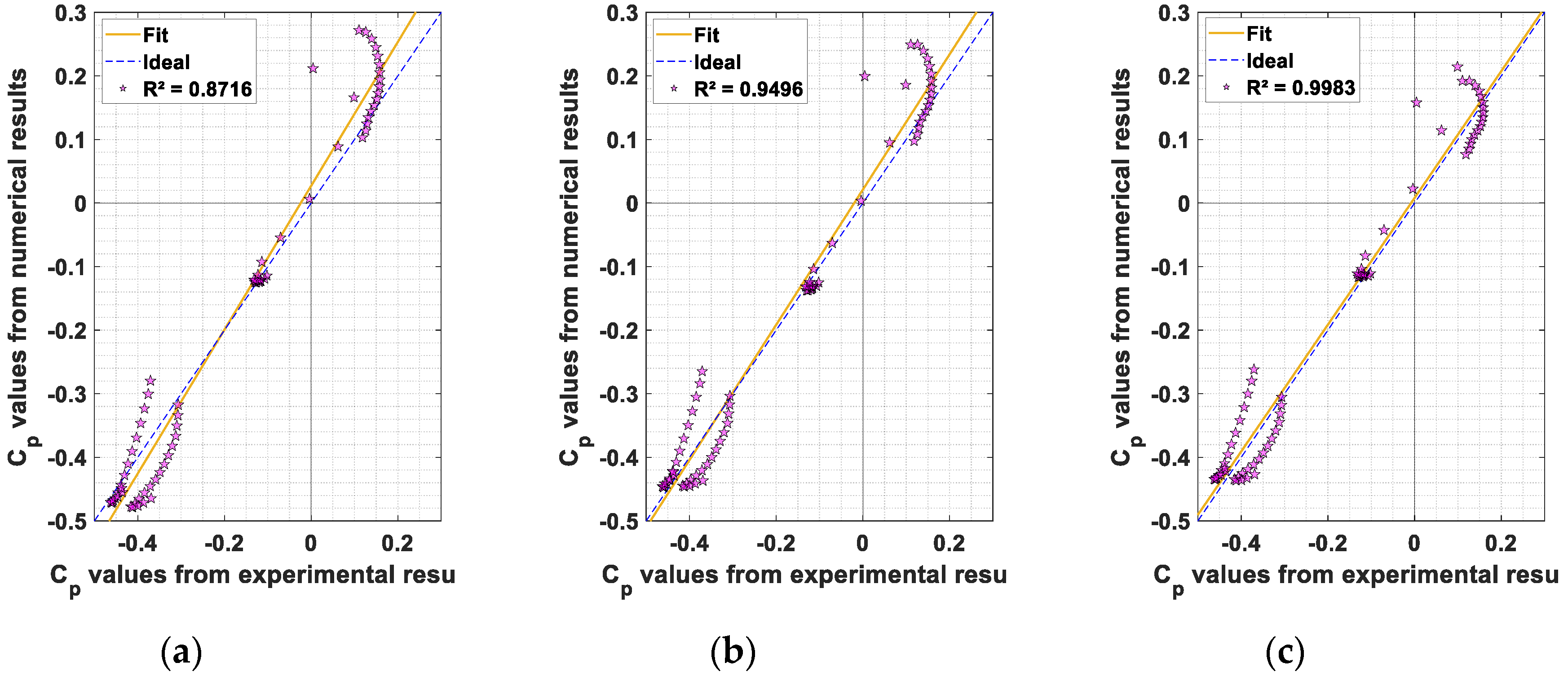
| 30° M1 | 1.132x + 0.027 | 0.8716 | 0.393 | 0.894 | 0.034 | 0.029 |
| 30° M2 | 1.063x + 0.021 | 0.9496 | 0.303 | 0.921 | 0.021 | 0.017 |
| 30° M3 | 0.997x + 0.008 | 0.9983 | 0.132 | 0.974 | 0.008 | 0.008 |
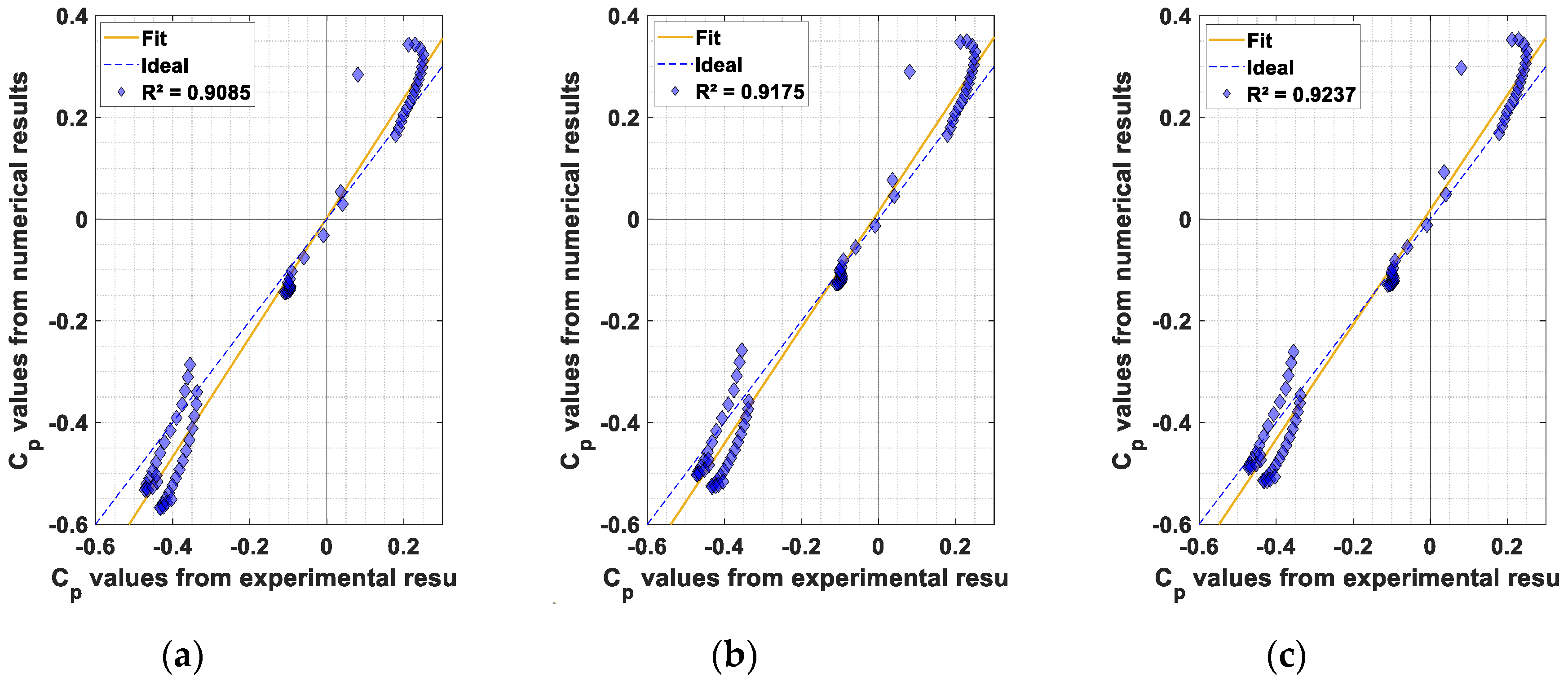
| 45° M1 | 1.174x + 0.002 | 0.9085 | 0.178 | 1.000 | 0.061 | 0.053 |
| 45° M2 | 1.141x + 0.015 | 0.9175 | 0.226 | 0.980 | 0.052 | 0.044 |
| 45° M3 | 1.128x + 0.018 | 0.9237 | 0.234 | 0.980 | 0.048 | 0.041 |
| Height | = 15° | = 30° |
|---|---|---|
| = 4 L |  |  |
| = 5 L |  |  |
| = 6 L |  |  |
| Legend | 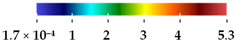 Velocity field | 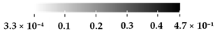 TKE field |
| Wind Angle | = 0 L | = 6 L |
|---|---|---|
| = 0° | 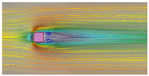 |  |
| = 15° | 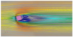 |  |
| = 30° |  |  |
| = 45° |  |  |
| Legend |  Velocity field |  TKE field |
Disclaimer/Publisher’s Note: The statements, opinions and data contained in all publications are solely those of the individual author(s) and contributor(s) and not of MDPI and/or the editor(s). MDPI and/or the editor(s) disclaim responsibility for any injury to people or property resulting from any ideas, methods, instructions or products referred to in the content. |
© 2025 by the authors. Licensee MDPI, Basel, Switzerland. This article is an open access article distributed under the terms and conditions of the Creative Commons Attribution (CC BY) license (https://creativecommons.org/licenses/by/4.0/).
Share and Cite
Silva, P.U.d.; Bono, G.; Greco, M. Application of Topology Optimization as a Tool for the Design of Bracing Systems of High-Rise Buildings. Buildings 2025, 15, 1180. https://doi.org/10.3390/buildings15071180
Silva PUd, Bono G, Greco M. Application of Topology Optimization as a Tool for the Design of Bracing Systems of High-Rise Buildings. Buildings. 2025; 15(7):1180. https://doi.org/10.3390/buildings15071180
Chicago/Turabian StyleSilva, Paulo Ulisses da, Gustavo Bono, and Marcelo Greco. 2025. "Application of Topology Optimization as a Tool for the Design of Bracing Systems of High-Rise Buildings" Buildings 15, no. 7: 1180. https://doi.org/10.3390/buildings15071180
APA StyleSilva, P. U. d., Bono, G., & Greco, M. (2025). Application of Topology Optimization as a Tool for the Design of Bracing Systems of High-Rise Buildings. Buildings, 15(7), 1180. https://doi.org/10.3390/buildings15071180