Thermal Mitigation in Coastal Cities: Marine and Urban Morphology Effects on Land Surface Temperature in Xiamen

Abstract

Amidst the rapid global urbanization and economic integration, coastal cities have undergone significant changes in urban spatial patterns. These changes have further worsened the complex urban thermal environment, making it crucial to study the interaction between human-driven development and natural climate systems. To address the insufficient quantification of marine elements in the urban planning of subtropical coastal zones, this study takes Xiamen, a typical deep-water port city, as an example to construct a spatial analysis framework integrating marine boundary layer parameters. This research employs interpolation simulation, atmospheric correction, and other techniques to simulate the inversion of land use and Landsat 8 data, deriving urban morphological elements and Land Surface Temperature (LST) data. These data were then assigned to 500 m grids for analysis. A bivariate spatial auto-correlation model was applied to examine the relationship between urban carbon emission and LST. The study area was categorized based on the influence of marine factors, and the spatial relationships between urban morphological elements and LST were analyzed using a multiscale geographically weighted regression model. Three Xiamen-specific discoveries emerged: (1) the marine exerts a significant thermal mitigation effect on the city, with an average influence range of 7.94 km; (2) the relationship between urban morphology and the thermal environment exhibits notable spatial heterogeneity across different regions; and (3) to mitigate urban thermal environments, connected green corridors should be established in the southern coastal areas of outer districts in regions significantly influenced by the ocean. In areas with less marine influence, spatial complexity should be introduced by disrupting relatively intact blue–green spaces, while regions unaffected by the ocean should focus on increasing green spaces and reducing impervious surfaces and water bodies. These findings directly inform Xiamen’s 2035 Master Plan for combating heat island effects in coastal special economic zones, providing transferable metrics for similar maritime cities.

1. Introduction

Global climate change not only poses significant challenges to human life but also profoundly impacts the urban thermal environment. With the acceleration of urbanization and the promotion of global economic integration, the expansion of urban space, increased building density, and diversified land use in coastal cities have led to continuous temperature rise in terrestrial areas [1,2]. The increase in temperature has caused droughts, heavy rainfall, fires, air pollution, and other extreme weather events, which have become major challenges in the daily lives of urban residents [3]. The thermal risk index in coastal cities is higher than that in inland cities [4], and the intensity of thermal risk significantly affects the sustainable development of coastal cities. Therefore, optimizing urban morphology in coastal cities is a key strategy for mitigating urban thermal environmental issues and promoting ecological civilization and green sustainable development.

In exploring ways to optimize urban morphology to alleviate the thermal environment, current research primarily uses indicators such as cooling intensity and cooling range [5] to investigate the cooling mechanisms of urban factors. These factors include park green spaces, ocean water bodies, and socio-economic elements. Regarding the cooling effects of green spaces and socio-economic factors, most studies analyze the correlation of park size [6,7,8] and shape [9], population exposure [10], land use changes [11], and three-dimensional indicators [12] with the thermal environment. These studies have demonstrated the spatial heterogeneity of the cooling effects of various urban elements. Compared to the research on green spaces and socio-economic factors, studies on the cooling effects of ocean water bodies are relatively scarce [13]. Most related research focuses on the cooling functions of river systems. For example, Hathway et al. [14] found that the cooling effect of rivers in the UK occurs only during the day; Cai et al. [15] discovered that rivers in Chongqing, China, can achieve a cooling range of up to 1 km; and Jiang et al. [16] found that the average cooling intensity of the Huangpu River ranges between 1.72 °C and 9.1 °C, with an average cooling range between 72.57 m and 465.42 m. These studies indicate that the mitigating effects of large water bodies (such as river systems) on the thermal environment exhibit gradient changes [17,18,19,20], and they confirm that water bodies are one of the key elements in alleviating urban thermal environments. As the largest and most extensive water body on Earth, the ocean provides a unique opportunity to mitigate urban heat island effects through the favorable coastal environment created by sea breezes [21], playing a crucial role in alleviating urban thermal environments [22]. Building on research on river water bodies, scholars have further analyzed and compared the differences in thermal environments between coastal and inland areas of cities, discovering spatial heterogeneity in LST between areas near and far from the coastline in coastal cities [23]. Additionally, recent studies have begun to focus on the thermal mitigation range of the ocean. For instance, Ossola et al. [24] found in their study of Los Angeles that the strongest cooling distance of the ocean is approximately 3 km; Guo et al. [25] discovered that the maximum cooling potential of seawater is within 2.5 km, with a maximum cooling range of 9.2 km; Chen et al. [22] further analyzed the ocean cooling range in coastal cities of the Yangtze River Delta across multiple seasons, finding that the ocean’s influence is greatest within 5 km of the coastline, with the most significant cooling effect in summer; and Shen et al. [26] proposed a new ocean cooling index as a way to explore the extent of ocean influence and cooling in Xiamen City.

In summary, current research on urban thermal mitigation has achieved a series of results. However, existing studies primarily focus on the cooling mechanisms of terrestrial urban factors, with limited research on the cooling effects of water bodies [13], particularly the key role of the ocean in mitigating thermal environments. Although some scholars have recently begun to study the cooling effects of the ocean, most of these studies use buffer zones to calculate changes in LST at different coastal distances, resulting in linear cooling ranges. However, due to the influence of urban morphology elements such as topography and buildings, different areas at the same distance may experience varying degrees of ocean influence, suggesting that the ocean’s cooling effects should exhibit nonlinear characteristics. Therefore, further research is needed to better understand the relationship between the ocean and urban thermal environments.

To fill these gaps, this study uses Xiamen as an experimental site, utilizes Landsat 8 to retrieve LST across Xiamen, and explores the ocean’s cooling range by comparing the relationship between urban carbon emission (UCE) and LST. Additionally, this study analyzes the optimization strategies of three urban morphology factors from a spatial perspective to achieve thermal mitigation goals. By deeply investigating the ocean’s impact on the urban thermal environment, this study aims to provide a more comprehensive understanding of Xiamen’s climate formation mechanisms and the evolution of its urban thermal environment, offering scientific support for urban planning and climate regulation in Xiamen. The main objective of this research is to comprehensively understand the complex relationship between urban morphology, carbon emissions, and the urban thermal environment in Xiamen. By doing so, we aim to achieve the following three tasks:

• Accurately retrieve LST across Xiamen using Landsat 8 data.
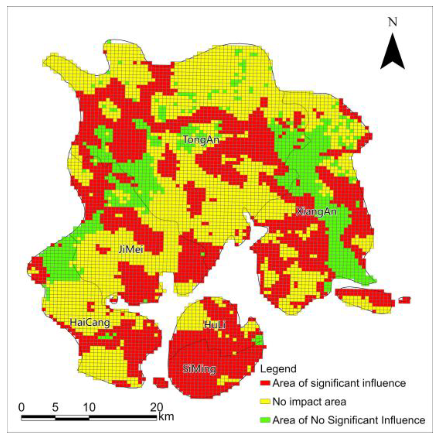
• Quantify relationship between UCE and LST and determine the ocean’s cooling range.
• Determine impact of three urban morphology factors (building density; green space ratio and water space ratio) on the urban thermal environment from a spatial perspective and propose corresponding optimization strategies.

2. Materials and Methods

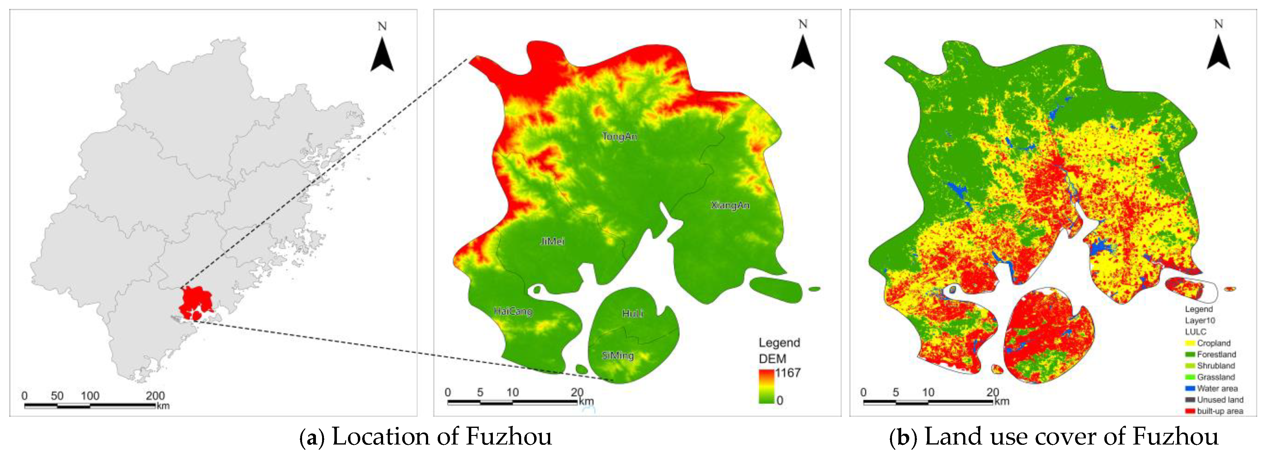
2.1. Study Area

Coastal cities, as vital hubs for international trade, not only enjoy more development opportunities but are also significantly influenced by marine climates. Xiamen, a key central city in southeastern China, is located in the southeastern part of Fujian Province, bordered by the Taiwan Strait to the east and the South China Sea to the south. The city comprises six districts: Tong’an, Xiang’an, Jimei, Haicang, Siming, and Huli (Figure 1).

Xiamen, situated on the southeast coast, features a south subtropical maritime monsoon climate. In spring, the temperature rises, with changeable weather and increasing rain and fog that impact heat diffusion. The summer is hot and rainy, with frequent typhoons and evident oceanic regulation. The autumn is cool and dry, with the northeast monsoon and cold dew wind affecting heat transfer. The winter is mild and dry, with occasional frost influencing urban heat storage. Its unique climate provides a basis for the study of the urban thermal environment. The city boasts abundant natural resources, including an excellent coastline and favorable climatic conditions, which provide advantageous conditions for urban development. The terrain features a mix of mountains, hills, and plains, but the overall topography is relatively flat, with no significant elevation changes, minimizing the impact of terrain on the ocean’s influence on the urban thermal environment. Over the past two decades, Xiamen’s built-up urban area has expanded from 160 km² to 405 km².

2.2. Materials

The data used in this study include Landsat 8 remote sensing images and NPP-VIIRS remote sensing images acquired on 30 January 2021. Additionally, this study references the research results of Yang et al. [27] on land use and land cover data. Land use data for China in 2021 with a spatial resolution of 30 m were selected. Post-processing, including cropping, was conducted to extract land use data within the study area. The land types were classified into eight categories: cropland, forest land, shrubland, grassland, water bodies, wetlands, built-up land, and unused land. Furthermore, nighttime light data for Fujian Province in 2021, nighttime light data for Xiamen in January, and energy consumption data for Fujian Province in 2021 were also utilized. The specific data sources are detailed in

Table 1. Data sources.

Data Name	Data Source
Boundary of the study area	Fujian Province Standard Map Service System, Approval Number: Min S(2023)254
Landsat remote sensing images within the study area	Geospatial Data Cloud, https://earthexplorer.usgs.gov/ (accessed on 10 September 2024)
Land use data within the study area	https://zenodo.org/record/5816591#.Y6ALbu2-uLU (10 September 2024)
Temperature within the study area	Inverted from Landsat8 images
Monthly and yearly NPP-VIIRS remote sensing data	https://eogdata.mines.edu/products/vnl/ (10 September 2024)
Energy consumption data in Fujian Province	China Energy Statistical Yearbook

.

2.3. Grid Study Area

A large number of grids were used as the sample in this study. The grid method allows for the reduction of large-scale macro data to a manageable sample size, making the quantified results more intuitive. Currently, both domestically and internationally, research on urban climate mostly divides urban land into grids of different scales for analysis [28,29,30]. For example, over 40 years of urban environmental climate research, conducted in in Stuttgart, Germany, has affirmed the rationality of using 500 m grids in regional-scale studies. Bottyán et al. studied the urban thermal environment of Debrecen using a 500 m grid scale [31], demonstrating that conducting urban climate research at this scale effectively explains urban characteristics. Furthermore, research on Beijing’s urban planning and meteorological environment suggests that a scale of 500 m to 4000 m is suitable for urban meteorological research and can better meet the needs of urban development [32,33]. Based on the research on these grid units mentioned above, this study gridified various types of data on Xiamen, selecting 500 m × 500 m square grids as the object of study.

2.4. Atmospheric Correction Method

Existing methods for retrieving LST primarily include atmospheric correction methods, single-channel algorithms, and split-window algorithms [34]. The atmospheric correction method can effectively eliminate the interference of satellite observation data due to atmospheric absorption, scattering, and other factors so as to more accurately obtain the real radiation information of the surface, which is crucial for the accurate inversion of the surface temperature. Thus, in this study, the atmospheric correction method is applied to invert the surface temperature of Landsat 8 data’s Band 10. The formula is as follows:

$$L_B=M_L\times DN+A_L$$

(1)

$$T_S={\displaystyle \frac{L_{\lambda }-L_{\uparrow }-\rho \left(1-\epsilon \right)L_{\downarrow }}{T\epsilon }}$$

(2)

$$LST={\displaystyle \frac{K_2}{\ln \left(K_1/T_S+1\right)}}-273.15$$

(3)

In the formula, L_B represents the thermal radiation intensity received by the satellite sensor, DN denotes the pixel grayscale value of Landsat 8’s Band 10, M_L and A_L are the gain and bias corresponding to the thermal infrared band, respectively, T_S stands for the radiance value of the black body, L_λ represents the radiance value of the thermal infrared radiation, ρ denotes the transmittance of the atmosphere in Band 10, ε, L_↑, and L_↓ represent the atmospheric emissivity, upward radiance, and downward radiance, respectively [35], for Landsat 8, K₁ = 774.89 (W·m⁻²·sr⁻¹·μm⁻¹), and K₂ = 1321.08 K [36].

2.5. Bivariate Spatial Auto-Correlation Model

Spatial auto-correlation analysis can measure whether variables exhibit spatial clustering on a spatial level. Based on this, Anselin [37] further proposed the bivariate spatial auto-correlation model, which can reveal the correlation between the attribute values of spatial units and those of neighboring spatial units, making it more suitable for urban areas with multiple attributes. In this study, the Local Indicators of Spatial Association (LISA) for UCE and LST of each grid sample point were analyzed using GeoDa software. The calculation formula is as follows [38]:

$$I_i=z_i{\displaystyle \sum _{j=1}^n{W}_{ij}{z}_j}$$

(4)

where I_i represents the local spatial relationship between the independent variable and the dependent variable in unit i, z_i and z_j are the variance-standardized values of observations in units i and j, and W_ij is the spatial weight matrix.

2.6. Carbon Emission Calculation

First, the direct carbon emission calculation results were obtained by summing the product of the area of each land use type and its respective carbon emission coefficient. The formula is as follows [39]:

$$E_c={{\displaystyle \sum C}}_i={\displaystyle \sum S_i}\cdot {\partial }_i$$

(5)

where E_c represents the direct carbon emissions, C_i denotes the carbon emissions produced by different land use types, S_i stands for the area of each land use type, and ∂_i represents the carbon emission (absorption) coefficient of each land use type, where positive values indicate carbon sources and negative values indicate carbon sinks. The carbon emission coefficients determined in this study were averaged from values derived from existing studies [39,40] and were used to determine the carbon emission coefficients for cropland, forest land, shrubland, grassland, water bodies, wetlands, and unused land (

Table 2. Carbon emission factors for various types of non-building land [40].

Land Use	Carbon Emission Coefficient	Unit
Cropland	0.0422	kg/(m2·a)
Forestland	−0.0578	kg/(m2·a)
Shrubland	−0.0578	kg/(m2·a)
Grassland	−0.0021	kg/(m2·a)
Water area	−0.0252	kg/(m2·a)
Wetland	−0.0252	kg/(m2·a)
Unused land	−0.0005	kg/(m2·a)

).

Next, the carbon emissions from construction land were calculated by summing the products of energy consumption for various types of energy and their respective carbon emission coefficients. The formula is as follows [40]:

$$E_{j1}={\displaystyle \sum E_{ji}}={\displaystyle \sum E_{ni}}\cdot {\theta }_i\cdot {\lambda }_i$$

(6)

where E_j1 represents the carbon emissions from construction land, E_ji denotes the carbon emissions from various types of energy, E_ni stands for the consumption of various types of energy, θ_i represents the coefficient for converting various types of energy to standard coal, and λ_i denotes the carbon emission coefficient for various types of energy. The values of θ_i, λ_i, and annual energy consumption are provided in

Table 3. Annual consumption of various types of energy and carbon emission conversion factors in Xiamen in 2021.

Year	Coal (104 t)	Coke (104 t)	Crude Oil (104 t)	Gasoline (104 t)	Kerosene (104 t)	Diesel (104 t)	Fuel Oil (104 t)	Natural Gas (106 m3)	Electricity (106 kWh)
θi	0.7143	0.9714	1.4286	1.4714	1.4714	1.4571	1.4286	1.2143	0.4040
λi	0.7559	0.8550	0.5857	0.5538	0.5714	0.5921	0.6185	0.4483	0.7935
2021	10,104.87	858.85	2839.74	540.19	117.24	429.63	189.03	60.04	2856.27

.

To spatially allocate such carbon emissions, this study utilized the brightness values (DN values) of NPP-VIIRS nighttime light data in Xiamen and the total DN value of nighttime light in Fujian Province in 2021 to estimate Xiamen’s indirect carbon emissions based on the total carbon emissions from energy consumption in Fujian Province. The formula is as follows [40]:

$$E_{j2}={\displaystyle \frac{DN}{TDN}}\times E_{j1}$$

(7)

where E_j2 represents the visualized carbon emission value, DN denotes the brightness value of NPP-VIIRS nighttime light, and TDN stands for the total brightness value of NPP-VIIRS nighttime light.

Finally, the total carbon emissions were calculated by summing the carbon emissions from construction land (indirect carbon emissions) and non-construction land (direct carbon emissions). The formula for calculating the total carbon emissions is as follows:

$$E_{total}=E_{j2}+E_c$$

(8)

where E_total represents the total carbon emissions, E_j2 denotes the carbon emissions from construction land (indirect carbon emissions), and E_c stands for the carbon emissions from non-construction land (direct carbon emissions).

2.7. Spatial Interpolation Method

To estimate the spatial distribution of carbon emissions in Xiamen, this study utilized spatial interpolation methods. Given that the carbon emissions from non-construction areas cannot be precisely located, the areal carbon emissions data were divided into numerous equally spaced carbon emission points. Then, spatial interpolation methods were used to estimate these unknown points. Common interpolation methods include Kriging, Inverse Distance Weighting (IDW), and spline interpolation. IDW is a local interpolation method that assumes unknown values are more influenced by nearby control points [41].

Considering the characteristics of carbon sources, which decrease in influence with distance, IDW was chosen for carbon emission interpolation. The formula for IDW interpolation is as follows:

$$L={\displaystyle \frac{{\displaystyle \sum _{i=1}^n\frac{1}{{(a_i)}^s}L({\mathrm{x}}_{\mathrm{i}})}}{{\displaystyle \sum _{i=1}^n\frac{1}{{(a_i)}^s}}}}$$

(9)

where L is the estimated carbon emission grid value, L(x_i) is the data of the i(i = 1, 2,…, n) carbon emission point, n is the number of points used for carbon emission interpolation, a_i is the distance from the interpolation point to the i-th carbon emission point, and a is the power of distance.

2.8. Multiscale Geographically Weighted Regression Model

Geographically weighted regression (GWR) can intuitively reflect the spatial relationships and strength of influence of analytical elements [42,43], but it cannot satisfy spatial localization analysis of multiple indicators. In this study, NDVI (Normalized Difference Vegetation Index), NDBI (Normalized Difference Built-up Index), and MNDWI (Modified Normalized Difference Water Index) were adopted as triadic indicators representing urban morphology. It is necessary to validate the respective impacts of these three indicators on the urban thermal environment. MGWR allows for different bandwidths among explanatory variables and calculates the bandwidth for each variable, thereby better accommodating the characteristics and intensity analysis of multivariate relationships. The bandwidth calculated by the MGWR model can serve as an indicator reflecting the scale of the explanatory variable’s effect. The formula is as follows [44]:

$$y_i={\beta }_0(u_i,v_i)+{\displaystyle \sum _{k=1}^m{\beta }_{bwk}(u_i,v_i)x_{ik}+{\epsilon }_i}$$

(10)

where (u_i, v_i) represents the coordinates of the sample points, β_bwk represents the regression coefficient for explanatory variable k, m is the number of sample points, bwk is the bandwidth, and ε_i is the error term of the model.

Comparing GWR and MGWR models for analyzing LST and urban morphology elements (

Table 4. Comparison of GWR model and MGWR model results.

		GWR Model	MGWR Model
Influenced area	R2	0.33	0.47
	Adjusted R2	0.23	0.36
	AICc	7012.75	6921.73
Area not significantly influenced	R2	0.87	0.88
	Adjusted R2	0.83	0.86
	AICc	1144.39	1009.47
Area not influenced	R2	0.91	0.91
	Adjusted R2	0.88	0.89
	AICc	2397.49	2263.29

AICc (Akaike Information Criterion, corrected): A criterion for model selection that evaluates the merit of a model by balancing the model’s fit to the data with the model’s complexity.

), the findings indicate that MGWR consistently outperforms GWR in terms of model fit across all regions. Specifically, in influenced areas, MGWR achieves a higher R² (R² = 0.47 > 0.33) and a higher adjusted R² (R² = 0.36 > 0.23), suggesting that it better captures spatial variations in LST. In areas with no significant influence, MGWR also slightly improves model performance (R² = 0.88 > 0.87), with a lower AICc (1009.47 > 1144.39), indicating a better balance between model complexity and goodness of fit. Even in areas with no influence, where both models show similar explanatory power (R² = 0.91), MGWR still achieves a lower AICc (2263.29 > 2397.49). These results highlight the advantages of MGWR in capturing spatial heterogeneity across different regions, making it a more robust approach for modeling the relationship between LST and urban morphology.

3. Results

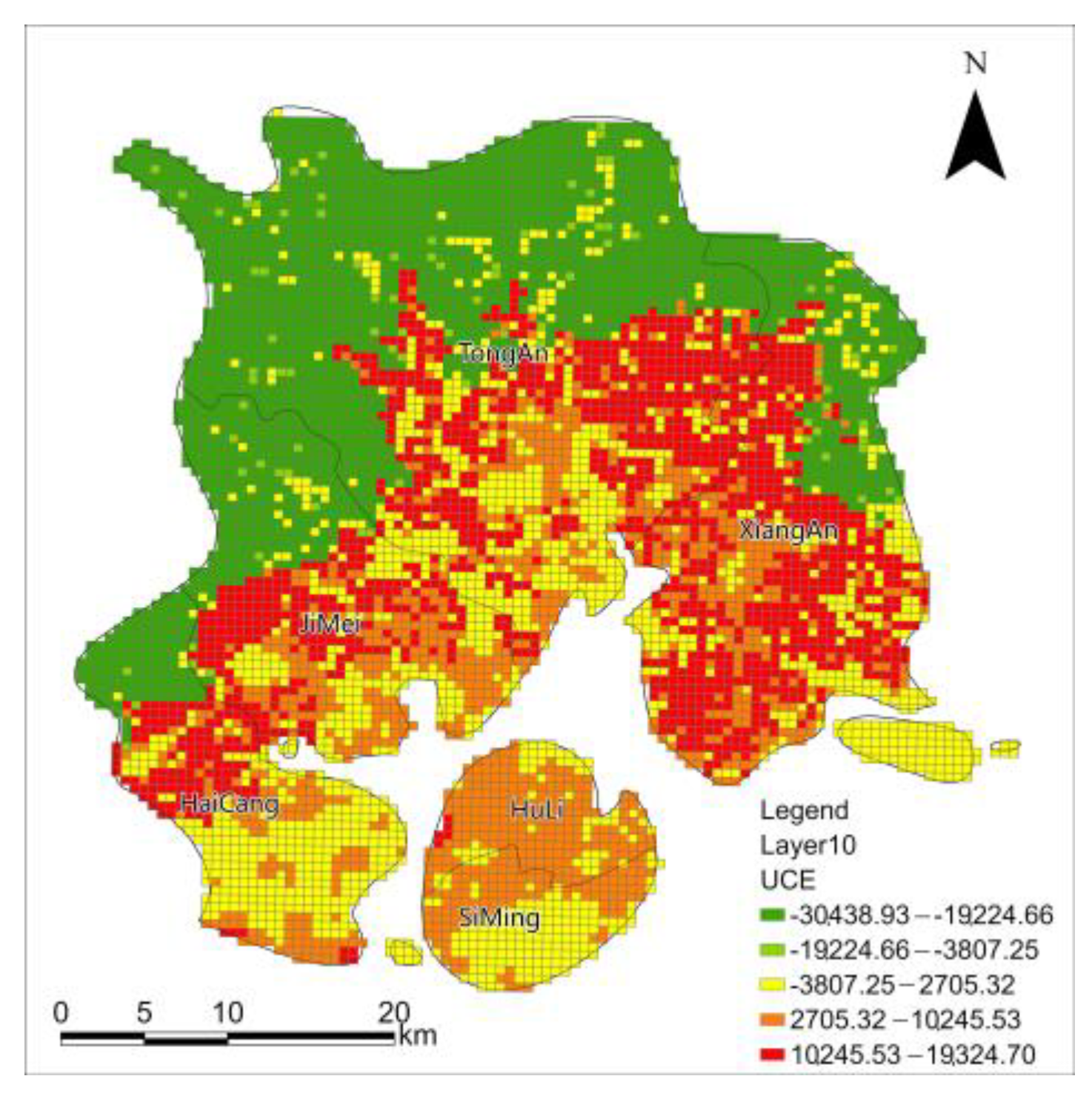
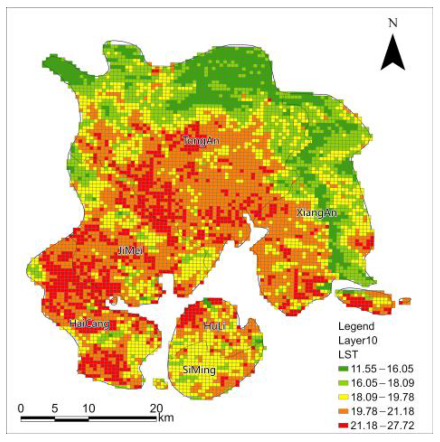
3.1. Spatial Distribution Characteristics of Carbon Emissions and Thermal Environment in Xiamen

The overall carbon emissions in Xiamen exhibit significant differences, with coastal areas showing much higher emissions than inland regions. Within the Xiamen municipality, areas like Huli District and Siming District, located on the islands, mostly fall within the carbon emission zones, which are closely associated with industrial activities and high traffic density. However, in specific areas such as Xiamen Botanical Garden and Dongping Mountain Park, a certain carbon sink effect is formed due to the intact mountain vegetation. This indicates that regions with high vegetation coverage and less human activity can possess strong carbon sink capabilities. This trend is also evident in the inland mountainous regions such as Jimei, Tong’an, Xiang’an, and Haicang, as depicted in Figure 2, where over eighty percent of the carbon sink exists in these areas.

Combined with socio-economic factors, the geographical location of these regions minimizes their exposure to human activities. Moreover, the high vegetation density in these areas promotes their role as urban carbon sinks. Additionally, the mountainous terrain acts as a natural barrier, reducing external carbon emissions and further facilitating the formation of carbon sink effects.

Regarding LST, Xiamen exhibited temperatures ranging from 11 °C to 28 °C on 30 January 2021, with a general trend of “lower in the north and higher in the south” (Figure 3). The high-temperature regions are located in the central and southern parts of Haicang, Jimei, and Tong’an and the southern part of Xiang’an. These areas, characterized by a high population density and intense construction activities, indicate that the intensity of socio-economic development and urban construction significantly influences LST.

Furthermore, examining the LST distribution in Huli District and Siming District reveals stark differences from other areas outside the islands. These regions exhibit relatively weaker thermal environments, mostly ranging from 18 °C to 20 °C. Despite the high population and construction densities in these areas, their spatial characteristics, surrounded by the sea with gentle terrain, indicate a direct influence of the ocean, highlighting the significant role of the ocean in influencing urban LST.

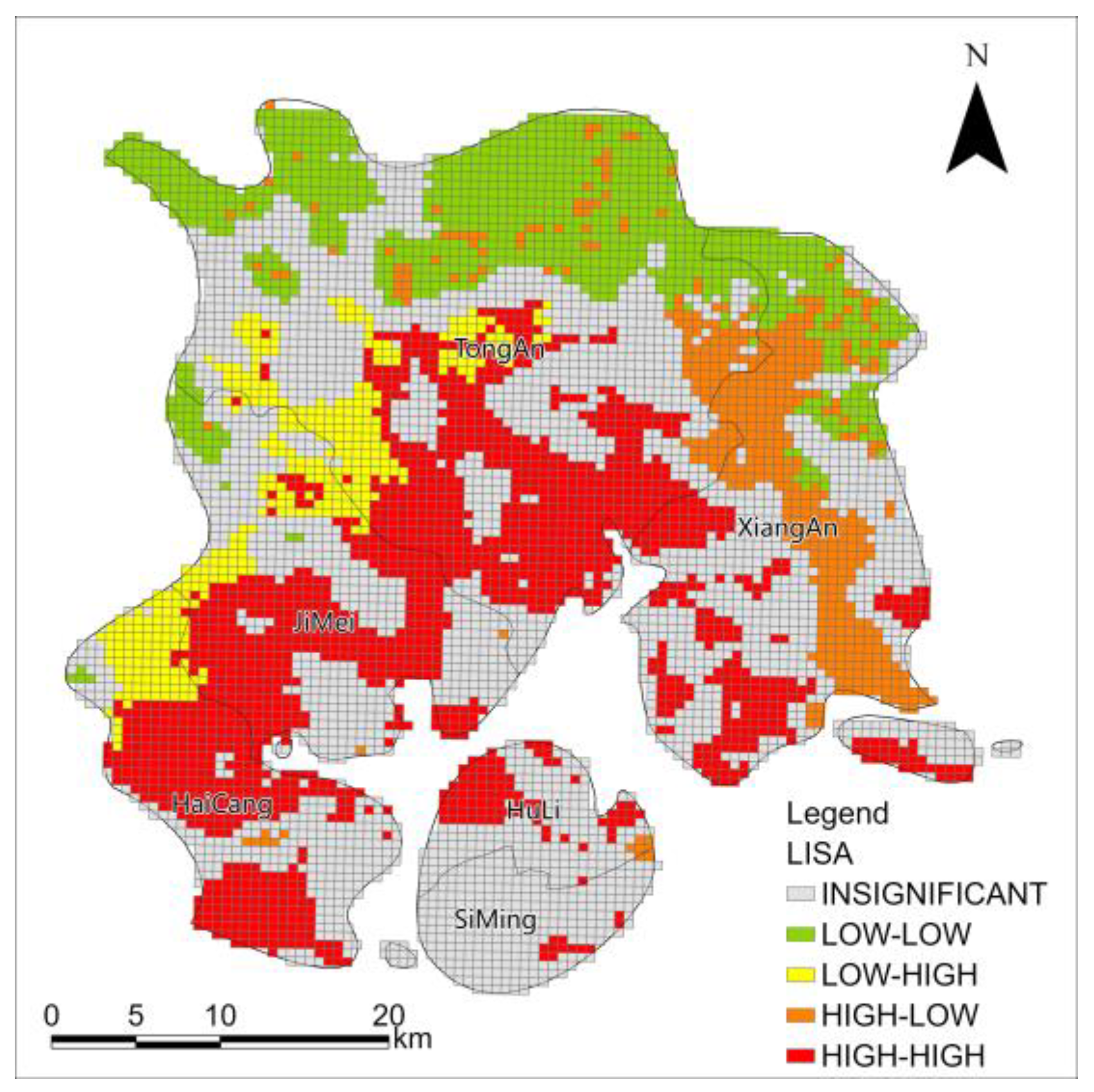
3.2. Bivariate Spatial Multivariate Correlation Between Carbon Emissions and Surface Temperature

The spatial auto-correlation between UCE and LST in Xiamen is categorized into five types: non-significant clustering areas, high–high clustering areas, low–low clustering areas, high–low clustering areas, and low–high clustering areas (Figure 4).

First, the non-significant clustering areas exhibit the largest extent, primarily distributed in the coastal regions both inside and outside the islands, as well as at the junction of urban and mountainous terrain. In these regions, the correlation between UCE and LST is weak, influenced by various factors, including marine regulation effects and topography. Second, the high–high and low–low clustering areas are relatively large in scale and best represent the positive correlation between UCE and LST. The high–high clustering areas indicate a strong correlation between high LST and high carbon emissions. In contrast, the low–low clustering areas reflect a correlation between low LST and low carbon emissions. Lastly, there are some low–high and high–low clustering areas. Low–high areas with predominantly cultivated land and high–low areas with extensive land–water interfaces suggest that factors such as cultivated land and land–water interfaces influence the relationship between UCE and LST to varying degrees. Additionally, the ocean is also a significant factor influencing the relationship between UCE and LST.

Previous studies have indicated that UCE increases with rising LST. However, bivariate spatial auto-correlation analysis of UCE and LST in Xiamen reveals complex regional differences in their relationship. Figure 5 shows that in certain areas of Xiamen, especially in most areas within the islands, the relationship between LST and UCE is not significant and may even exhibit negative correlations. This phenomenon is closely related to the geographical characteristics of the region, particularly its coastal location. These areas are influenced by marine regulation, resulting in weak correlations between LST and UCE.

To gain a deeper understanding of this influence, this study divides the overall region of Xiamen into three categories to explain the differences in the relationship between LST and UCE. First, areas where LST is unrelated to UCE are categorized as being influenced by the ocean. The modulation of these areas by marine climate results in a weak association between LST and UCE. Second, areas classified as having no significant influence include both high–low and low–high clustering areas, where the relationship between LST and UCE is disturbed by other factors, preventing the formation of substantial correlations. Lastly, areas classified as having no influence include high–high and low–low clustering areas, where the relationship between LST and UCE is stable and not influenced by external factors. The distribution of these three categories of areas is illustrated in Figure 5.

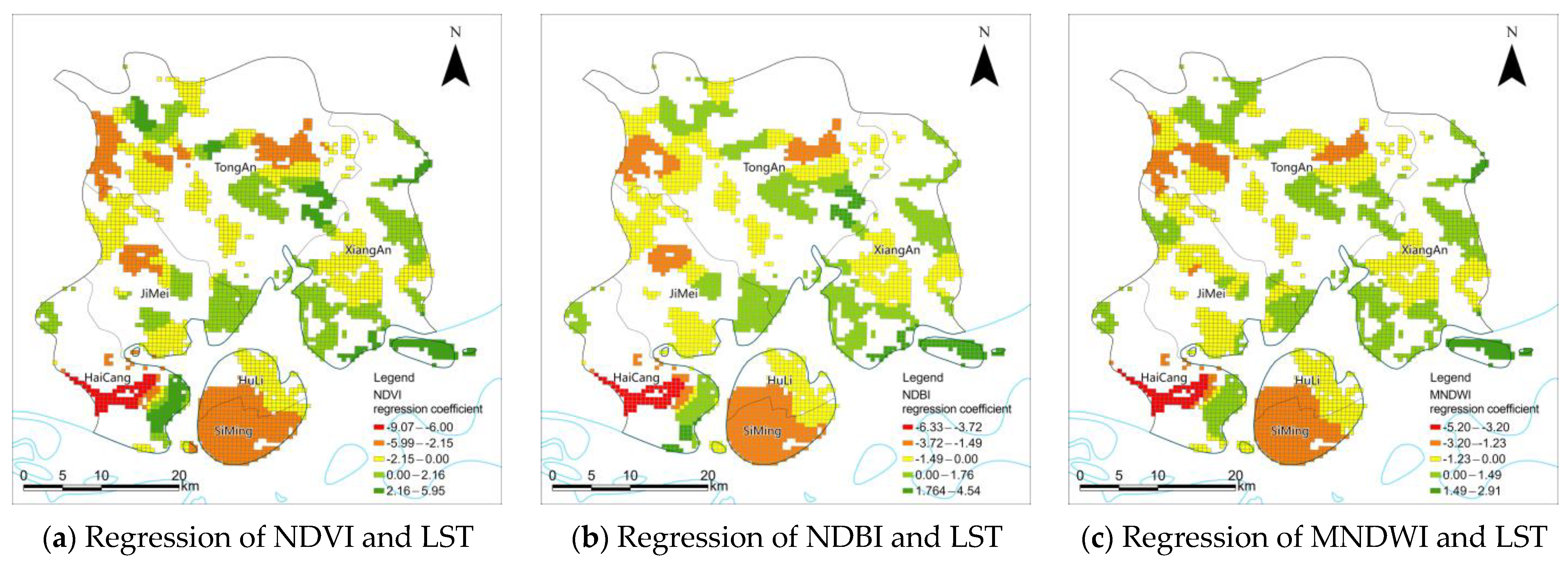
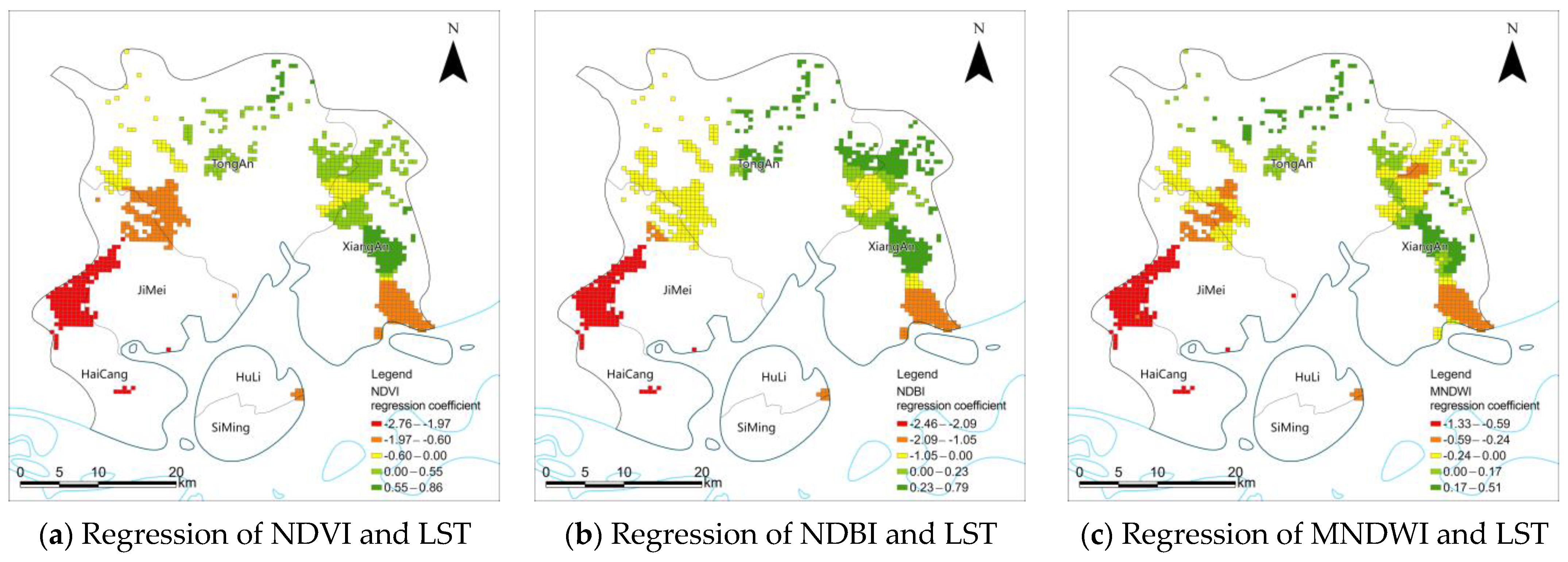
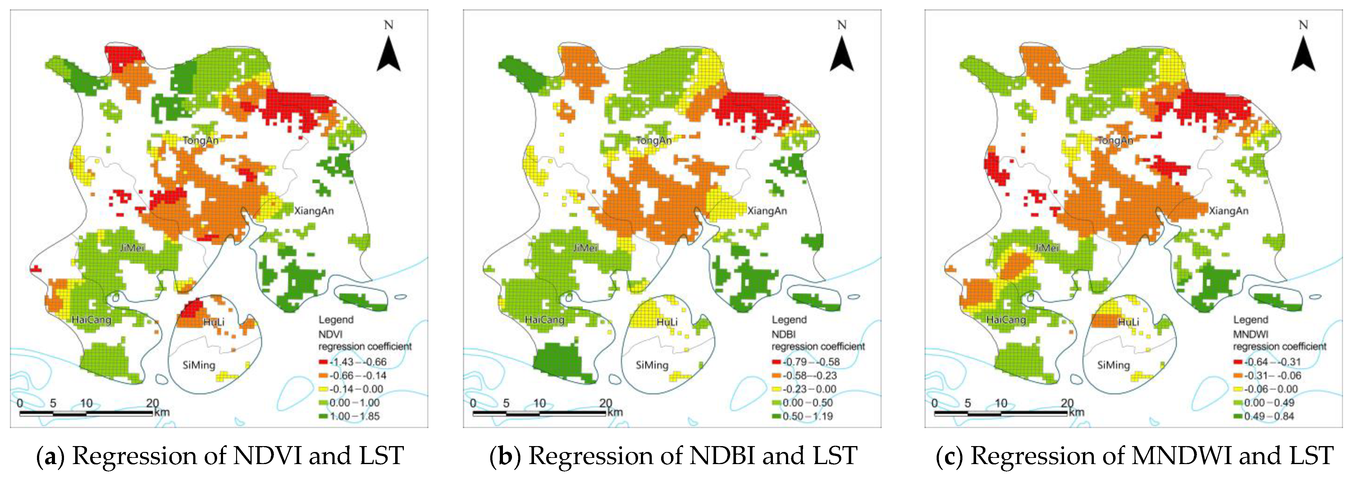
3.3. Spatial Variability in the Relationship Between Urban Form and Thermal Environment Correlations

Based on the sub-regional results (Figure 6 and

Table 5. Correlation between LST and urban morphological factors in areas with different impacts from the ocean.

			NDVI	NDBI	MNDWI
Areas significantly influenced by the ocean	LST	Pearson Correlation	−0.147 **	0.156 **	0.043 *
		p-value	0.000	0.000	0.028
		Cases	2649	2649	2649
Areas less significantly influenced by the ocean	LST	Pearson Correlation	0.659 **	−0.696 **	0.074 *
		p-value	0.000	0.000	0.025
		Cases	921	921	921
Areas non-significantly influenced by the ocean	LST	Pearson Correlation	−0.730 **	0.706 **	0.401 **
		p-value	0.000	0.000	0.000
		Cases	2743	2743	2743

** Significant at the 0.01 level (two-tailed). * Significant at the 0.05 level (two-tailed).

), to further explore the specific numerical proportions of the correlations between various urban elements and LST, this study employed a multiple regression model to analyze the relationships between different urban morphological factors and LST. The aim was to derive more actionable strategies for thermal mitigation. During this process, it was observed that NDVI, NDBI, and MNDWI exhibit high multicollinearity. To ensure the rationality of the regression results, the least significant factor correlated with LST, i.e., MNDWI, was excluded from the multiple regression analysis.

According to Figure 7, in areas significantly influenced by the ocean, the multiple regression equation is as follows:

$$LST=19.68-0.46\times NDVI+2.43\times NDBI$$

(11)

This indicates that in these regions, increasing vegetation coverage and decreasing construction intensity are necessary to achieve effective thermal mitigation. For instance, a 0.1 increase in vegetation density and a 0.1 decrease in construction intensity can result in a 0.3 °C temperature reduction. Further analysis reveals that reducing construction intensity has a more pronounced cooling effect than increasing vegetation density.

In areas with less ocean influence, the multiple regression equation is as follows:

$$LST=15.84+1.63\times NDVI-29.84\times NDBI$$

(12)

Here, construction intensity is the urban morphological factor with the most significant negative impact on LST. This suggests that moderately increasing construction intensity and appropriately reducing vegetation coverage can be beneficial in this region. Moreover, increasing construction intensity alone yields better cooling effects than reducing vegetation coverage alone. Calculations show that a 0.1 decrease in vegetation coverage and a 0.1 increase in construction intensity can achieve a 3 °C cooling effect.

In areas without ocean influence, the multiple regression equation is as follows:

$$LST=22.58-14.53\times NDVI+9.89\times NDBI$$

(13)

In this case, vegetation coverage has a negative correlation with LST, while construction intensity has a positive correlation. The negative impact of vegetation coverage on LST is greater than the positive impact of construction intensity. Therefore, greater emphasis should be placed on integrating vegetation coverage in these regions. Numerically, a 0.1 increase in vegetation coverage and a 0.1 decrease in construction intensity can collectively reduce LST by 2.4 °C.

Comparing the multiple regression fitting curves across the three regions, the slope of the curve in areas with significant ocean influence is the flattest. Further analysis of the R² values reveals that the R² of the multiple regression model in areas with significant ocean influence is only 0.02, significantly lower than that in areas with less ocean influence (R² = 0.48) and areas without ocean influence (R² = 0.54). This pattern of slope flattening and the gradual increase in R² as ocean influence diminishes suggest that the ocean significantly affects the thermal mitigation roles of urban morphological factors such as NDVI and NDBI.

The Pearson coefficient of IBM SPSS Statistics 27 and the MGWR model of ArcGIS Pro 3.0.1 were used to perform the correlation analysis between urban elements and thermal environment in three types of areas and the correlation was dropped for green spaces; it was found that the correlation in different areas had more obvious differences.

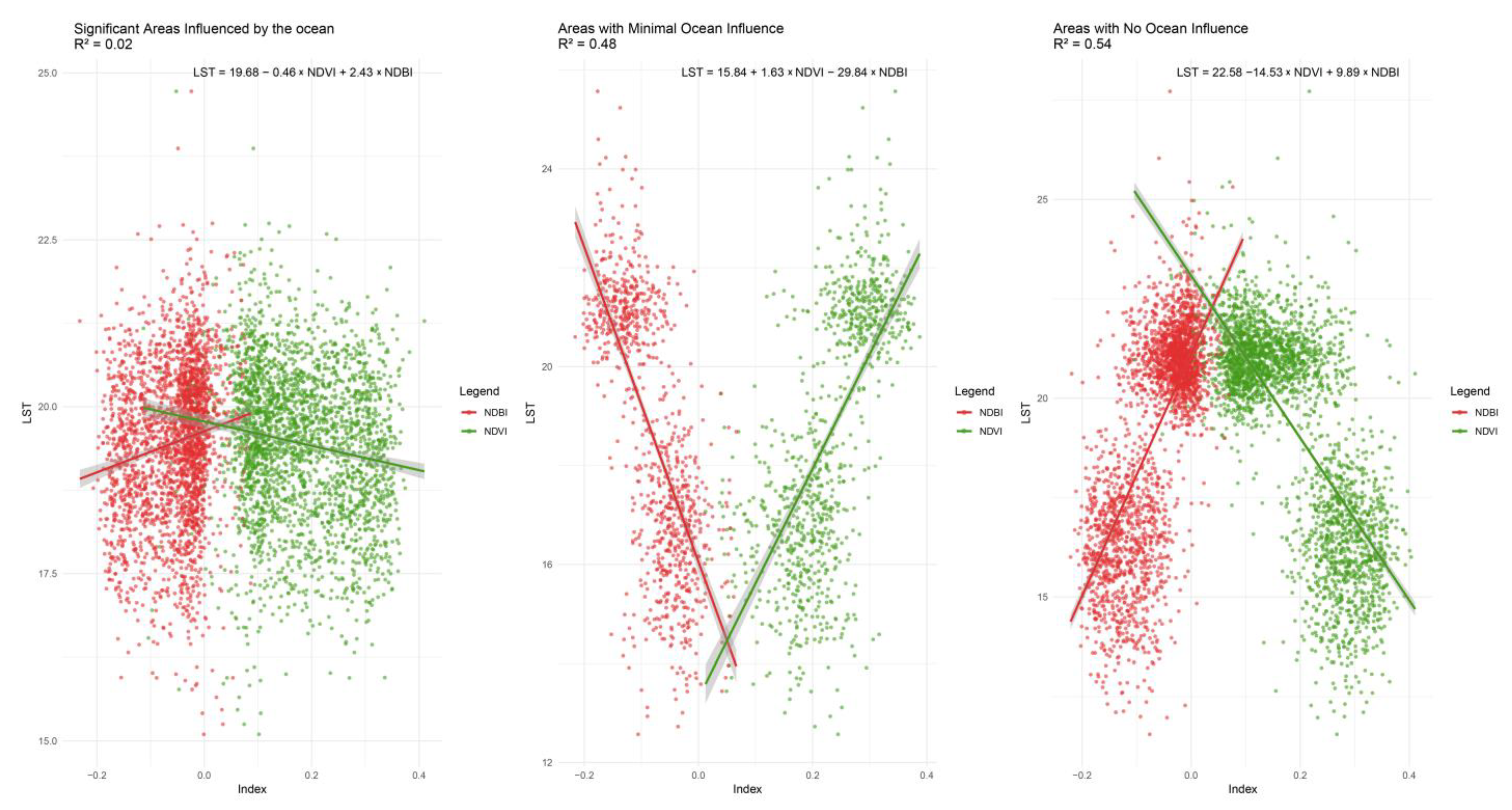
3.3.1. Ocean-Influenced Areas: Urbanization Overrides Vegetation and Water Cooling

Within the areas of Xiamen City that are highly influenced by the sea, the characteristics of the spatial distribution are critical to the relationship between surface temperature and vegetation cover, building density, and water distribution (Table 5). These areas tend to show a clear intertwining of urbanization and the natural environment, and their spatial structure influences the distribution pattern of surface temperature.

First, LST showed a highly significant negative correlation with NDVI. Considering the distribution of vegetation in the coastal area of Xiamen, in the city center area, and in the suburbs, the vegetation cover is relatively small and mainly occupied by human activities such as buildings and roads, resulting in higher surface temperatures. In the suburbs or coastal areas, on the other hand, there is more vegetation cover due to the presence of natural environments such as mountain woodlands, parks, and green spaces, as well as coastal vegetation zones, resulting in relatively lower surface temperatures.

Second, LST shows a highly significant positive relationship with NDBI. This significant relationship is emphasized in Huli and Siming Districts, which are the main urban areas of Xiamen, with a dense layout of high-rise buildings and commercial areas and a large amount of man-made materials, such as concrete, covering the surface, which results in high heat production capacity and relatively high surface temperatures.

Finally, there is a significant positive correlation between LST and MNDWI, which reflects that the distribution of water bodies in the coastal area of Xiamen City has a more complex effect on surface temperature. The general view is that water bodies have a certain cooling effect, which can alleviate the heat in the surrounding area. However, in the coastal zone, which is strongly influenced by the ocean, the ocean possesses a large heat capacity and can absorb a large amount of heat, which plays a certain role in regulating the thermal environment inland. Therefore, in such areas, the mitigating effect of water bodies influenced by the ocean climate on surface temperature may not be as significant as inland areas or may even show a certain positive correlation.

According to Table 5, only NDVI has a highly significant negative correlation with the thermal environment, while NDBI has a highly significant positive correlation with the thermal environment and a significant positive correlation with MNDWI, indicating that appropriately reducing the scale of construction land and waters and increasing the perfect vegetation cover will help the thermal mitigation in the areas affected by the ocean. From Figure 7, it can be found that the correlation strength between the three types of urban elements and the thermal environment is weaker in the island of Xiamen, the southern part of the Haicang District, and part of the mountainous waters in the Tong’an District, while the correlation strength is stronger in the southern coastal areas of the districts and counties outside the island. The analysis shows that for the areas close to the mountains, the green land pattern itself is complete, and even if the NDVI is increased further, it cannot significantly improve the strength of the local thermal environment. For the island area of Xiamen City, due to the continuous increase in water and construction land, the building land is dense and compact, and although the park green space has been increased in recent years, the distribution is fragmented and poorly connected, which greatly destroys the connectivity of the blue–green space, and will lead to the intensification of the thermal environment; it is more difficult to propose thermal mitigation strategies from the aspect of the urban form, which has been proven by a number of studies [45,46,47].

3.3.2. Areas Less Influenced by the Ocean: Stronger Building Cooling Effect

According to the results in Table 5, LST showed a highly significant positive correlation with NDVI. This means that areas with more vegetation cover usually have lower surface temperatures in the study area. This spatial relationship may reflect the characteristics of urban or suburban areas that are rich in green spaces, such as parks, forestland, or farmland. Vegetation in these areas reduces surface temperatures by absorbing solar radiation and evapotranspiration, creating a relatively cool microclimate.

On the contrary, LST showed a highly significant negative correlation with NDBI, indicating higher surface temperatures in built-up areas. This suggests that in urban centers or commercial areas, the centralized arrangement of a large number of buildings leads to high heat capacity and absorption capacity, which results in higher surface temperatures. In addition, hard surfaces such as roads and sidewalks also absorb and release heat, exacerbating the heat island effect in these areas.

As for the weaker but still significant correlation between LST and MNDWI, it shows that the presence of water bodies has a positive relationship with surface temperature. Although water bodies usually mitigate surface temperatures, in urban environments, where the influence of the sea is not significant and where the construction intensity is moderate, i.e., smaller than in the main urban areas but larger than in areas such as mountains and woodlands, the role of water in heat mitigation is relatively weak.

According to the analysis results in Table 5, it was found that in the regions less affected by the ocean, LST shows a positive correlation with NDVI and MNDWI (especially the correlation with NDVI, which is extremely significant), while it shows highly significant negative correlation with NDBI. This suggests that a moderate break in the integrity of the blue–green space can significantly alleviate thermal environmental problems in these regions. This finding is consistent with the findings of Tingting Hong et al. that increasing the complexity of patches within the green space system can enhance the localized cooling effect of the city [42].

Further observation of the correlation strength characteristics visualized by the MGWR regression model (Figure 8) reveals that the correlation strength of the three types of urban elements with the thermal environment as a whole shows a trend of gradual strengthening from southwest to northeast. This implies that in the northeastern part of Xiamen City (e.g., the northeastern part of Tong’an District), an appropriate amount of breaking up of blue and green spaces would provide greater thermal mitigation. Adding impervious surfaces of appropriate scale in these areas will help to further expand the extent of urban construction and promote urban development.

3.3.3. Areas Not Influenced by the Ocean: Vegetation Cooling Dominates

The relationship between LST and NDVI, NDBI, and MNDWI reflects the influence of urban spatial patterns on surface temperature. First, LST and NDVI showed a negative correlation, i.e., areas with more vegetation cover had lower surface temperatures. This phenomenon illustrates the importance of increasing the appropriate amount of green space coverage and protecting ecosystems in the urban planning process, which can regulate the urban thermal environment and improve the comfort of the city and its ability to adapt to climate change.

Second, the positive correlation between LST and NDBI indicates that the surface temperature is higher in densely built-up areas. This suggests that urban planning needs to pay attention to factors such as building layout, density, and materials and take effective urban heat island management measures, such as increasing green roofs and improving building insulation performance, in order to mitigate the negative impacts of the urban heat island effect on human health and the urban ecosystem.

Finally, the positive correlation between LST and MNDWI indicates that water bodies have a certain regulatory effect on surface temperature. In this regard, in the planning and design of cities, it is necessary to rationally lay out water bodies and water systems and utilize the thermoregulatory effect of water bodies to improve the urban thermal environment, which is essential for increasing the comfort of urban landscapes and human habitation. However, it should be noted that the regulating effect of water bodies on surface temperature may be affected by the artificial structure of the city and the type of land use; so, the location, size, and surrounding environment of urban water bodies need to be considered comprehensively in the planning and design.

The correlations shown in Table 5 are further spatially located (Figure 9), and it is not difficult to find that the correlations between the three types of urban form elements and the thermal environment are weaker in the south and east of Tong’an District, which indicates that the adjustment of urban elements in these areas has less impact on the thermal environment and that, according to the actual land use, the construction density of this area is too high and there is less ecological land, which cannot realize urban heat mitigation due to various social, economic, and demographic factors. This means that the thermal environment is less affected by the adjustment of urban elements in these areas. According to the actual land use situation, the construction density in this area is too high, and the ecological land is too small; so, urban heat mitigation cannot be realized from the adjustment of urban morphology due to various social, economic, and demographic factors.

4. Discussion

4.1. Spatial Impact Range of Ocean on Thermal Environment

This study identifies that the ocean’s influence on Xiamen’s thermal environment extends approximately 7.94 km inland on average. The spatial analysis reveals that the regulatory effect of the ocean is not confined to coastal areas but also extends to inland regions. This implies that in urban planning processes, attention should be paid not only to thermal environment issues in coastal areas but also to other factors affecting the thermal environment in inland areas. Therefore, when formulating urban planning heat mitigation strategies, it is necessary to consider the impact range of the ocean’s regulation of the thermal environment to ensure effective heat reduction in the urban environment.

Furthermore, the ocean’s influence on the thermal environment does not follow a simple linear pattern but exhibits fluctuations due to various factors such as wind intensity and urban topography. These natural factors are relatively difficult to modify in urban development. Therefore, adjusting urban morphological factors becomes an important means of heat mitigation. By adjusting urban morphological factors such as vegetation density, water body density, and building density, the regulatory effect of the ocean’s thermal regulation can effectively mitigate the degree of the urban heat island effect.

4.2. Spatial Differences in Urban Morphological Factors Under Ocean Influence

According to Table 4 and Table 5, it is evident that there are significant differences in the influence of the ocean on urban morphological factors in different regions. In areas with significant ocean influence, the correlation between surface temperature vegetation coverage and building density is relatively weak. Conversely, in areas with less ocean influence, the opposite trend is observed, while in areas unaffected by the ocean, similar phenomena are observed. These differences between different regions are closely related to factors such as geographical location, climatic conditions, and urban development patterns.

Specifically, in areas with significant ocean influence, the weak correlation between surface temperature and vegetation coverage and building density is due to the regulatory effect of the ocean, which stabilizes the climatic conditions in the area, thereby weakening the correlation between surface temperature and vegetation coverage and building density. Conversely, in areas with less ocean influence, due to the weaker regulatory effect of the ocean, vegetation coverage and building density have a more direct impact on surface temperature. Areas unaffected by the ocean are more affected by inland climatic conditions or socio-economic factors, leading to a more evident correlation of vegetation coverage and building density with surface temperature.

In summary, these results provide important clues for understanding the mechanism of urban thermal environment formation and the mode of action of ocean heat mitigation. Understanding the differences in heat mitigation methods between coastal cities and inland cities helps to formulate targeted urban planning and climate control strategies, thereby more effectively mitigating the urban heat island effect and improving the quality of the urban ecological environment.

4.3. Urban Morphology Optimization Strategies for Thermal Mitigation Goals

4.3.1. Ocean-Influenced Areas: Establishing Green Corridors in Southern Coastal Regions

Given the findings presented in Figure 8, enhancing the connectivity of park green spaces in coastal areas is a crucial strategy for improving the urban thermal environment. Establishing interconnected green corridors can facilitate better airflow and temperature regulation. Additionally, rational planning of water spaces such as lakes, river systems, and artificial water bodies in various districts and counties—for example, reducing the water body area within the island, particularly in northern regions—may enhance the overall thermal equilibrium. Furthermore, optimizing construction land density in the island area of Xiamen by adjusting spatial layouts can effectively improve the urban heat environment.

4.3.2. Areas Less Influenced by the Ocean: Enhancing Spatial Complexity in Tong’an District

According to Figure 9, in areas less influenced by the ocean, the thermal environment can be effectively improved by rationally utilizing urban factors such as NDVI and MNDWI. Specifically, in the northeastern part of Xiamen (e.g., the northeastern part of Tong’an District), moderately disrupting blue–green spaces can have a greater thermal mitigation effect. Additionally, increasing the proportion of impervious surfaces in these areas can not only alleviate thermal environmental intensity but also contribute to further urban expansion and development. Therefore, future urban planning and construction should focus on greening and water body utilization in these regions to achieve more sustainable and livable urban development goals. Moreover, urban development inevitably involves construction, and the results of this study indicate that construction in these areas will yield better thermal mitigation effects compared to other regions.

4.3.3. Areas Not Influenced by the Ocean: Green Space Expansion and Impervious Surfaces Reduction in Outer Island Regions

Table 5 highlights a strong correlation between urban morphological factors and the thermal environment in inland areas unaffected by the ocean. Specifically, a negative correlation exists with NDVI, meaning that as green space coverage increases, the intensity of the thermal environment decreases. Conversely, positive correlations exist with NDBI and MNDWI, indicating that increases in construction land density and water body density exacerbate the thermal environment. Based on these findings, prioritizing green space expansion while reducing impervious surfaces and excess water bodies is recommended for optimal heat mitigation. As demonstrated in Figure 9, this approach can be implemented by reducing impervious surface areas in Haicang, Jimei, and Xiang’an Districts and converting them into parklands or forests. Additionally, parts of the water spaces in Xiang’an District, central Jimei District, and southern Haicang District can be transformed into park green spaces.

5. Conclusions

This study utilized a synergistic approach integrating remote sensing data analysis and advanced statistical techniques. Specifically, high-resolution satellite imagery was processed to compute indices like the Normalized Difference Vegetation Index (NDVI), the Normalized Difference Built-up Index (NDBI), and the Modified Normalized Difference Water Index (MNDWI), followed by correlation and regression analyses. By employing these methods, this study solved the problem of comprehensively elucidating the impact of marine factors on the urban thermal environment and exploring the intricate relationships between diverse urban factors and the thermal environment.

This study considers the influence of marine factors on the urban thermal environment and reveals that the spatial scope of marine regulation is not linearly confined to coastal areas but extends to some extent into inland regions. This provides a new perspective on previous research and offers fresh insights into the mechanisms underlying urban thermal environments. Second, by analyzing the relationships between urban factors (such as vegetation cover, building density, and water body coverage) and the thermal environment, this study uncovers the extent and manner in which different factors influence the thermal environment. Notably, this study finds that the water body coefficient in coastal cities exhibits a positive correlation with the thermal environment, which differs from conclusions drawn in studies of inland cities. This finding highlights that the cooling effect of the ocean is more pronounced than that of rivers and lakes in coastal cities. Finally, based on the research results, targeted urban planning recommendations are proposed for different regions to effectively mitigate thermal environmental issues. For instance, in areas significantly influenced by the ocean, it is essential to construct interconnected green corridors in the southern coastal regions of outer districts and counties.

The research is of great significance for urban planning and environmental management. It reveals a nonlinear spatial pattern of marine influence on the urban thermal environment, where the ocean’s influence extends into inland regions. The discovery of distinct impacts of different urban factors on the thermal environment, especially the prominent oceanic cooling effect in coastal cities, provides crucial insights for urban planners. This knowledge can be used to optimize urban design, enhance urban thermal comfort, and mitigate the negative impacts of urban heat islands, thus contributing to more sustainable urban development.

However, this study has some limitations. First, due to data accuracy and calculation errors, there may be discrepancies in the conclusions drawn for different regions, which could affect a comprehensive understanding of the ocean’s impact on the thermal environment. Second, Xiamen was chosen as the study area because its coastal terrain is predominantly flat, eliminating the influence of topography on ocean temperature regulation. However, the generalizability of the findings to coastal cities with varied topography may be limited. Lastly, the urban morphological factors selected for this study include NDVI, NDBI, and MNDWI, but socio-economic factors were not considered, which may result in incomplete conclusions.

Based on these limitations, the following strategies can be adopted in the future:

• For coastal cities with complex topographies, future research should be dedicated to developing customized urban planning strategies that account for the intricate interactions between topography and the ocean in shaping the thermal environment. This may involve the use of numerical simulation models to predict the thermal environment under different topographic and urban design scenarios.
• In terms of data collection and analysis, future studies should strive to amass more comprehensive datasets, including high-resolution remote sensing data with multi-spectral and multi-temporal information, as well as detailed socio-economic data at the neighborhood level. Such comprehensive data will enable more accurate modeling and prediction of the urban thermal environment, thereby providing a robust scientific basis for evidence-based urban planning and management.

References

1. Oke, T.R. The energetic basis of the urban heat island. Quart. J. R. Met. Soc. 1982, 108, 1–24. [Google Scholar] [CrossRef]
2. Zhu, E.; Qi, Q.; Chen, L.; Wu, X. The spatial-temporal patterns and multiple driving mechanisms of carbon emissions in the process of urbanization: A case study in Zhejiang, China. J. Clean. Prod. 2022, 358, 131954. [Google Scholar] [CrossRef]
3. Sun, R.; Lü, Y.; Yang, X.; Chen, L. Understanding the variability of urban heat islands from local background climate and urbanization. J. Clean. Prod. 2019, 208, 743–752. [Google Scholar] [CrossRef]
4. Morabito, M.; Crisci, A.; Gioli, B.; Gualtieri, G.; Toscano, P.; Di Stefano, V.; Gensini, G.F. Urban-hazard risk analysis: Mapping of heat-related risks in the elderly in major Italian cities. PLoS ONE 2015, 10, e0127277. [Google Scholar] [CrossRef]
5. Chang, C.R.; Li, M.H. Effects of urban parks on the local urban thermal environment. Urban For. Urban Green. 2014, 13, 672–681. [Google Scholar] [CrossRef]
6. Cao, X.; Onishi, A.; Chen, J.; Imura, H. Quantifying the cool island intensity of urban parks using ASTER and IKONOS data. Landsc. Urban Plan. 2010, 96, 224–231. [Google Scholar] [CrossRef]
7. Cheng, X.; Wei, B.; Chen, G.; Li, J. Influence of park size and its surrounding urban landscape patterns on the park cooling effect. J. Urban Plan. Dev. 2015, 141, A4014002. [Google Scholar] [CrossRef]
8. Qiu, K.; Jia, B. The roles of landscape both inside the park and the surroundings in park cooling effect. Sustain. Cities Soc. 2020, 52, 101864. [Google Scholar] [CrossRef]
9. Chen, M.; Dai, F. The influence of urban green spaces on thermal environment based on morphological spatial pattern analysis. Ecol. Environ. Sci. 2021, 30, 125–134. (In Chinese) [Google Scholar]
10. Wei, C.; Wan, Y.; Huang, G.; Zhou, L.; Chang, Y. Spatiotemporal characteristics of heatwaves and population exposure in coastal cities of China. Remote Sens. Technol. Appl. 2024, 39, 679–689. (In Chinese) [Google Scholar]
11. Zhao, Q.; Peng, J.S. Spatiotemporal characteristics of land use and thermal environment in the built-up area of Shizong County. Agric. Technol. 2024, 44, 84–90. [Google Scholar]
12. Li, T.; Huang, X.; Guo, H.; Hong, T. Contribution and Marginal Effects of Landscape Patterns on Thermal Environment: A Study Based on the BRT Model. Buildings 2024, 14, 2388. [Google Scholar] [CrossRef]
13. Ruiz, M.A.; Colli, M.F.; Martinez, C.F.; Correa-Cantaloube, E.N. Park cool island and built environment. A ten-year evaluation in Parque Central, Mendoza-Argentina. Sustain. Cities Soc. 2022, 79, 103681. [Google Scholar] [CrossRef]
14. Hathway, E.A.; Sharples, S. The interaction of rivers and urban form in mitigating the Urban Heat Island effect: A UK case study. Build. Environ. 2012, 58, 14–22. [Google Scholar] [CrossRef]
15. Cai, Z.; Han, G.; Chen, M. Do water bodies play an important role in the relationship between urban form and land surface temperature? Sustain. Cities Soc. 2018, 39, 487–498. [Google Scholar] [CrossRef]
16. Jiang, L.; Liu, S.; Liu, C.; Feng, Y. How do urban spatial patterns influence the river cooling effect? A case study of the Huangpu Riverfront in Shanghai, China. Sustain. Cities Soc. 2021, 69, 102835. [Google Scholar] [CrossRef]
17. Declet-Barreto, J.; Knowlton, K.; Jenerette, G.D.; Buyantuev, A. Effects of urban vegetation on mitigating exposure of vulnerable populations to excessive heat in Cleveland, Ohio. Weather. Clim. Soc. 2016, 8, 507–524. [Google Scholar] [CrossRef]
18. Wang, Y.; Ouyang, W. Investigating the heterogeneity of water-cooling effect for cooler cities. Sustain. Cities Soc. 2021, 75, 103281. [Google Scholar] [CrossRef]
19. Kirschner, V.; Moravec, D.; Macku, K.; Kozhoridze, G.; Komárek, J. Comparing the effects of green and blue bodies and urban morphology on land surface temperatures close to rivers and large lakes. Land 2024, 13, 162. [Google Scholar] [CrossRef]
20. Zhou, W.; Wu, T.; Tao, X. Exploring the spatial and seasonal heterogeneity of cooling effect of an urban river on a landscape scale. Sci. Rep. 2024, 14, 8327. [Google Scholar] [CrossRef]
21. Lan, H.N.; Lau, K.K.L.; Shi, Y.; Ren, C. Improved urban heat island mitigation using bioclimatic redevelopment along an urban waterfront at Victoria Dockside, Hong Kong. Sustain. Cities Soc. 2021, 74, 103172. [Google Scholar] [CrossRef]
22. Chen, L.; Qi, Q.; Wu, H.; Feng, D.; Zhu, E.Y. Will the landscape composition and socio-economic development of coastal cities have an impact on the marine cooling effect? Sustain. Cities Soc. 2023, 89, 104328. [Google Scholar] [CrossRef]
23. Al-Ruzouq, R.; Shanableh, A.; Khalil, M.A.; Zeiada, W.; Hamad, K.; Abu Dabous, S.; Gibril, M.B.A.; Al-Khayyat, G.; Kaloush, K.E.; Al-Mansoori, S.; et al. Spatial and temporal inversion of land surface temperature along coastal cities in Arid Regions. Remote Sens. 2022, 14, 1893. [Google Scholar] [CrossRef]
24. Ossola, A.; Jenerette, G.D.; McGrath, A.; Chow, W.; Hughes, L.; Leishman, M.R. Small vegetated patches greatly reduce urban surface temperature during a summer heatwave in Adelaide, Australia. Landsc. Urban Plan. 2021, 209, 104046. [Google Scholar] [CrossRef]
25. Guo, F.; Zhao, J.; Zhang, H.; Dong, J.; Zhu, P.; Lau, S.S.Y. Effects of urban form on sea cooling capacity under the heatwave. Sustain. Cities Soc. 2023, 88, 104271. [Google Scholar] [CrossRef]
26. Shen, Y.; Zhang, Q.; Liu, Q.; Huang, M.; Yao, X.; Jiang, K.; Ke, M.; Ren, Y.; Zhu, Z. The Impact of Urban Spatial Forms on Marine Cooling Effects in Mainland and Island Regions: A Case Study of Xiamen, China. Sustain. Cities Soc. 2025, 121, 106210. [Google Scholar] [CrossRef]
27. Yang, J.; Huang, X. The 30 m annual land cover dataset and its dynamics in China from 1990 to 2019. Earth Syst. Sci. Data 2021, 13, 3907–3925. [Google Scholar] [CrossRef]
28. Chen, M.; Dai, F. Effects of Urban Green Infrastructure Spatial Pattern on PM2.5 Based on MSPA. Chin. Landsc. Archit. 2020, 36, 63–68. (In Chinese) [Google Scholar]
29. Chen, G.; Chen, H.; Chen, Z.; Zhang, B.; Shao, L.; Guo, S.; Zhou, S.; Jiang, M. Low-carbon building assessment and multi-scale input-output analysis. Commun. Nonlinear Sci. Numer. Simul. 2011, 16, 583–595. [Google Scholar] [CrossRef]
30. Bottyán, Z.; Unger, J. A multiple linear statistical model forest imating the mean maximum urban heat island. Theor. Appl. Climatol. 2003, 75, 233–243. [Google Scholar] [CrossRef]
31. Balázs, B.; Unger, J.; Gál, T.; Sümeghy, Z.; Geiger, J.; Szegedi, S. Simulation of the mean urban heat island using 2D surface parameters: Empirical modelling, verification and extension. Meteorol. Appl. 2009, 16, 275–287. [Google Scholar] [CrossRef]
32. Ren, C.; Wu, E. Climate Maps for Urban Environments: An Information System tool for Sustainable Urban Planning; China Architecture Industry Press: Beijing, China, 2012; pp. 35–65. (In Chinese) [Google Scholar]
33. Yang, X.; Gao, W.; Fu, F.; Li, S. Research on Multi-scale Influence Mechanism Visualization and Countermeasures of Climate Environment Sensitivity in Urban Administrative Regions-A Case Study of Fengtai District in Beijing. Chin. Landsc. Archit. 2022, 38, 51–56. (In Chinese) [Google Scholar]
34. Liu, B.; Bao, G.; Peng, K.; Shi, M.; He, H. Comparison of Different Land Surface Temperature Algorithms Based on Landsat TMlmages. J. Spatio-Temporal Inf. 2015, 22, 57–61. (In Chinese) [Google Scholar]
35. Zhao, H.; Alimujiang, K. Study on the relationship between thermal environment and underlying surface in the main urban area of Úrümgi. Sci. Surv. Mapp. 2021, 46, 179–187. (In Chinese) [Google Scholar]
36. Xie, Z.; Huang, T.; Li, Y.; Liu, Y.; Wu, D.; Wang, H. Study on the Relationship between Spatial-Temporal Evolution of Land Use and of Urban Heat Environment in Nanchang. Environ. Sci. Technol. 2019, 42, 241–248. (In Chinese) [Google Scholar]
37. Anselin, L. Local indicators of spatial association–LISA. Geogr. Anal. 1995, 27, 93–115. [Google Scholar]
38. Çelebioğlu, F. Regional disparity and clusters in Turkey: A Lisa (Local Indicators of Spatial Association) analysis. Dumlupınar Üniversitesi Sos. Bilim. Derg. 2010, 28, 35–47. [Google Scholar]
39. Cui, Y.; Li, L.; Chen, L.; Zhang, Y.; Cheng, L.; Zhou, X.; Yang, X. Land-use carbon emissions estimation for the Yangtze River Delta Urban Agglomeration using 1994–2016 Landsat image data. Remote Sens. 2018, 10, 1334. [Google Scholar] [CrossRef]
40. Hong, T.; Huang, X.; Zhang, X.; Deng, X. Correlation modelling between land surface temperatures and urban carbon emissions using multi-source remote sensing data: A case study. Phys. Chem. Earth Parts A/B/C 2023, 132, 103489. [Google Scholar] [CrossRef]
41. Wang, J. Comparison of inverse distance weights and Tyson polygon spatial interpolation in the modeling of soil benzo(a)pyrene exceedance areas. Sci. Technol. Vis. 2021, 15, 28–30. (In Chinese) [Google Scholar] [CrossRef]
42. Hong, T.; Huang, X.; Deng, X.; Yang, Y.; Tang, X. Study on the Relationship between Urban Green Infrastructure and Thermal Environment Based on Morphological Spatial Pattern Analysis—A Case Study of Central Urban Area of Fuzhou City. Chin. Landsc. Archit. 2023, 39, 97–103. (In Chinese) [Google Scholar]
43. Hong, T.; Huang, X.; Chen, G.; Yang, Y.; Chen, L. Exploring the spatiotemporal relationship between green infrastructure and urban heat island under multi-source remote sensing imagery: A case study of Fuzhou City. CAAI Trans. Intell. Technol. 2023, 8, 1337–1349. [Google Scholar] [CrossRef]
44. Hu, J.; Zhang, J.; Li, Y. Exploring the spatial and temporal driving mechanisms of landscape patterns on habitat quality in a city undergoing rapid urbanization based on GTWR and MGWR: The case of Nanjing, China. Ecol. Indic. 2022, 143, 109333. [Google Scholar] [CrossRef]
45. Chen, Y.; Liu, W.; Rong, Y.; Fu, L.; Ma, L.; Cao, Y. Habitat quality assessment of the Datong Beichuan River Source Nature Reserve based on land use and vegetation coverage. Res. Soil Water Conserv. 2020, 27, 332–337+393. [Google Scholar]
46. Zhou, T.; Liu, H.; Gou, P.; Xu, N. Conflict or coordination? Measuring the relationships between urbanization and vegetation cover in China. Ecol. Indic. 2023, 147, 109993. [Google Scholar] [CrossRef]
47. Li, Q.; Hu, X.; Wei, B.; Zhang, Y.; Chen, C.; Liu, L. Study on the coupling relationship between green space and urban expansion in Changsha City. Econ. Geogr. 2022, 42, 87–94. [Google Scholar] [CrossRef]
Figure 1. Location and land cover use of the central Fuzhou District.
Buildings 15 01170 g001
Figure 2. Distribution of UCE.
Buildings 15 01170 g002
Figure 3. Distribution of LST.
Buildings 15 01170 g003
Figure 4. Bivariate spatial auto-correlation clustering analysis of LST and UCE.
Buildings 15 01170 g004
Figure 5. Map of areas classified by the degree of marine influence.
Buildings 15 01170 g005
Figure 6. Multiple regression modeling of urban form elements and LST in different marine-influenced areas.
Buildings 15 01170 g006
Figure 7. MGWR regression analysis of urban morphology and thermal environment in areas with significant marine influence.
Buildings 15 01170 g007
Figure 8. MGWR regression analysis of urban morphology and thermal environment in areas with minor marine influence.
Buildings 15 01170 g008
Figure 9. MGWR regression analysis of urban morphology and thermal environment in areas without marine influence.
Buildings 15 01170 g009