Calculating the Bearing Capacity of Foundations near Slopes Based on the Limit Equilibrium and Limit Analysis Methods

Abstract

The ultimate bearing capacity of foundations near slopes is a widely discussed and researched topic in the field of geotechnics. Using the plane strain strength equation of the limit equilibrium and limit analysis methods, we established a new model for calculating the bearing capacity of foundations near slopes that can consider the intermediate principal stress, horizontal distance from the foundation to the shoulder of the slope, and roughness of the base. A formula of the ultimate bearing capacity of the foundation of foundations near slopes was derived, compared, and analyzed with that of finite element analysis software and other calculation methods. Comparative analysis was carried out using finite element analysis software and other calculation methods, and it was found that the obtained results are closer to the real solution of the ultimate bearing capacity of foundations near slopes. The intermediate principal stresses can improve the bearing capacity of foundations near slopes. The bearing capacity of foundations near slopes increases with the horizontal distance from the foundation to the slope and then remains constant. The results of this study can better reflect the actual ultimate bearing capacity of foundations near slopes and have certain theoretical significance for the optimal design of foundations near slopes.

1. Introduction

In the field of infrastructure development, such as roads, railroads, buildings, power, and water projects, it is common to encounter situations where work needs to be carried out on foundations close to or on slopes. These foundations can be categorized into two types: foundations close to slopes (referred to as slope-facing foundations) and foundations on slopes (referred to as slope foundations) [1,2]. Both types fall into the same category of slope foundations. For example, when constructing a high-grade highway in a mountainous area, a large number of high-fill embankments need to be built on slope-adjacent foundations; when a railroad crosses a highway, the foundation of the bridge often needs to be constructed on a sloping roadbed; and when constructing a dam in a gully area or carrying out a construction project in a mountainous area, the foundation needs to be constructed on a sloping foundation.

In these cases, improper construction locations may lead to engineering disasters such as landslides. Landslides and large deformations during construction are not only safety hazards but may also seriously threaten the safety of people’s lives and property. They cause major economic losses and may lead to serious social problems. Therefore, strict design and construction standards must be adopted for these engineering constructions to ensure the stability and safety of the projects.

At present, various methods such as the limit equilibrium method [3,4,5,6,7,8], slip line method [9,10,11,12,13], limit analysis method [14,15,16,17,18,19,20,21], and numerical simulation method [22,23] are mainly used to calculate and analyze the bearing capacity of foundations on adjacent slopes directly from these slopes. The current state of domestic and international research is as follows: recently, Baazouzi et al. [24] used the finite difference software FLAC 2D to investigate the foundation bearing capacity of strip foundations on or near a slope under inclined loads, and their study showed that the shape of the interaction diagram between vertical and horizontal loads was related to the distance of the foundation from the shoulder of the slope and the angle of the slope. Kusakabe, O. et al. [25] derived an upper limit solution for the bearing capacity of a pro-slope foundation using a unilateral sliding damage model consisting of three slides, assuming that the triangular wedge under the strip foundation is symmetric. Yang, X. L. et al. [26,27] obtained cohesion, overload, and gravity bearing coefficients for different slope inclinations based on the energy dissipation method of plastic mechanics using a multi-wedge translation damage mechanism, with the coefficient of the bearing capacity is given in the form of a design graph. Yang, X. L. et al. [28] analyzed the damage mechanism of slope-facing foundations and divided the foundation damage into slope face damage, foot of slope damage, bottom of slope damage, and top of slope damage, obtaining the dimensionless expressions of cohesion, overload, and gravity bearing capacity coefficients. Zhao Luo et al. [29] and Yang Feng et al. [30] constructed a multi-slider two-dimensional maneuvering permit damage model and a grid-like rigid slider system containing nonlinear constraints, respectively, and obtained the upper limit solution of the bearing capacity of the pro-slope foundation. Casablanca O [31] used the MATLAB program to prepare an upper limit method finite element program to analyze and study the extreme damage of foundations on adjacent slopes or slopes and established the objective function and mathematical planning model, obtaining the analytical solution of the bearing capacity of foundation on the adjacent slope and slope. El Sawwaf et al. [32,33] investigated the potential benefits of reinforcing the replaced sand layer near the top of the slope. The depth of the replaced sand layer and the location of the toe of the slope relative to the top of the slope were discussed for several parameters based on model tests. A series of finite element analyses were also carried out to validate the prototype slope using a two-dimensional plane strain model, and critical values of geogrid parameters were determined to achieve maximum reinforcement.

To avoid building collapse, most researchers use pile foundations or other forms of deep foundations for their research. In addition, they improve and reinforce the foundation sufficiently for safety reasons. For example, Faghihmaleki, H. [34] showed that metakaolin and microsilica fume enhanced the strength of concrete using experiments with different control groups. Bagheri Kalaye, A. [35] discussed the effect of irregularities in the analytical design of house structures in the case of earthquake induced design irregularities. Bararpour, M. [36] studied the effect of these fibers on both plain and volcanic ash concrete and proved that the use of polypropylene fibers reduces the compressive strength of concrete. However, this practice not only increases the project’s cost but is also difficult to implement. These approximations, such as treating them as horizontal foundations or discounting the bearing capacity of the foundations merely based on experience, lack scientific justifications, and the results may be too conservative or have insufficient safety reserves. If the ultimate bearing capacity of slope foundations can be calculated accurately and the stability of slope foundations can be analyzed reasonably, this problem can be effectively solved.

In summary, scholars have analyzed the deformation damage mechanism of foundations adjacent to slopes by establishing models for tests; through the study of slip line field theory, they have established the damage modes of foundations adjacent to slopes and carried out calculations on foundations adjacent to slopes. However, the existing research is still insufficient in the following aspects: 1. Numerical simulation software: the research on the damage mode and deformation evolution mechanism under each working condition is not comprehensive enough, which makes it difficult to prevent and monitor the damage behavior of the adjacent slopes’ foundations in the actual engineering; 2. Ultimate bearing capacity calculation: the influence of various factors on the ultimate bearing capacity (such as the slope angle, the distance from the foundation to the slope, etc.) is not taken into account, which leads to the limitation of the calculated results. Therefore, it is necessary to carry out an in-depth study on the deformation evolution of foundations adjacent to slopes under different working conditions and the calculation of ultimate bearing capacity under the influence of different factors.

2. Analysis of the Basic Influencing Factors of Foundations near Slopes

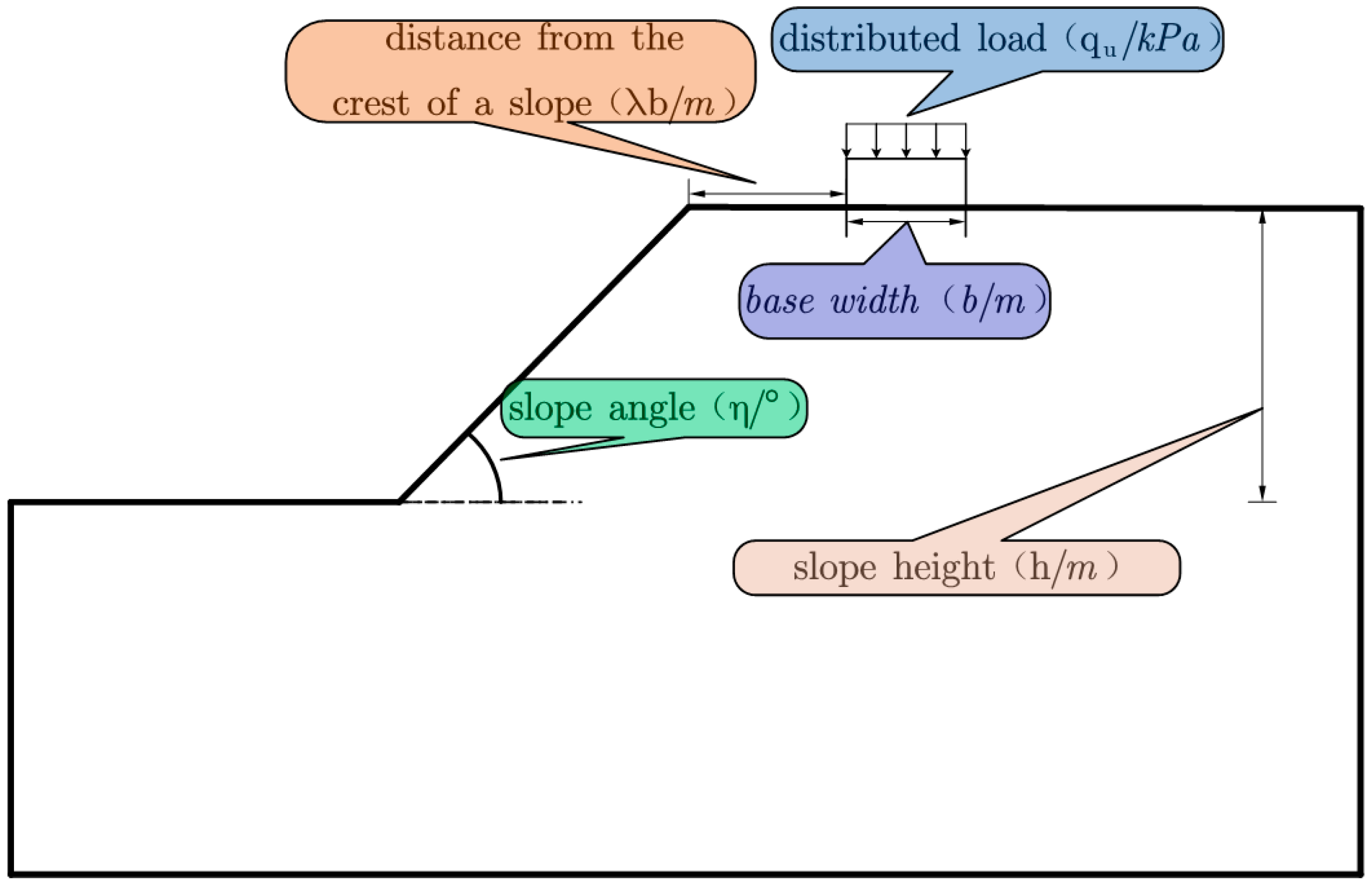
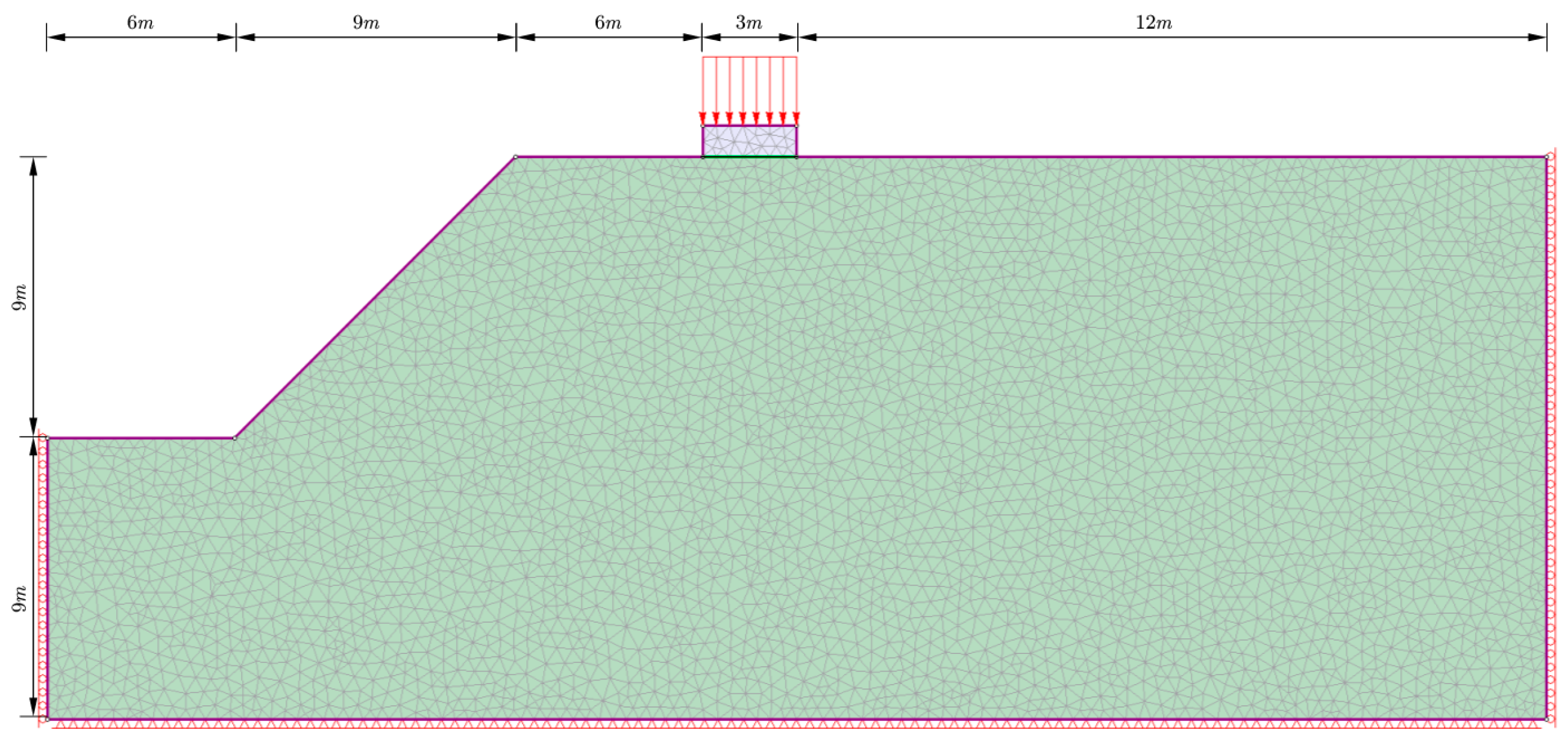
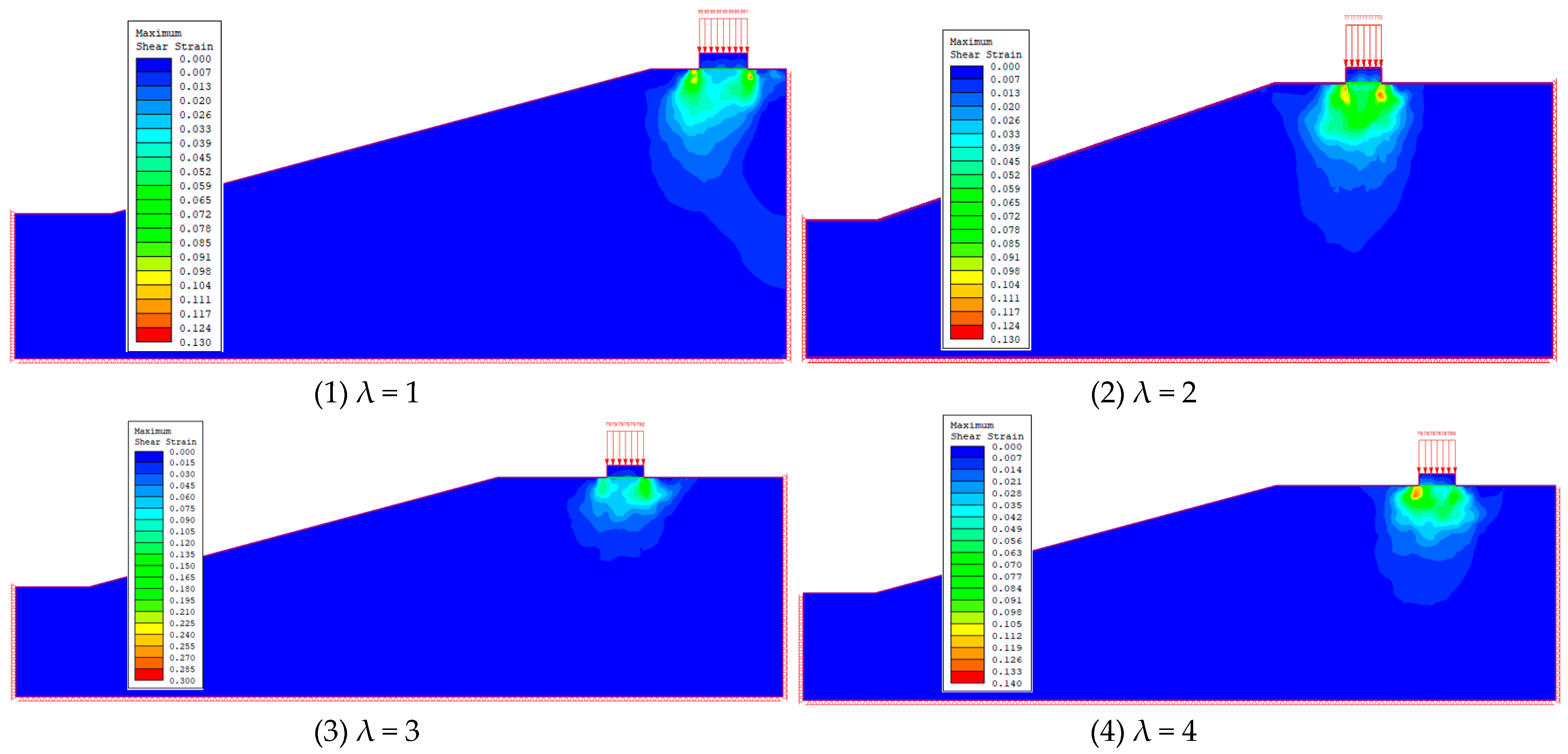
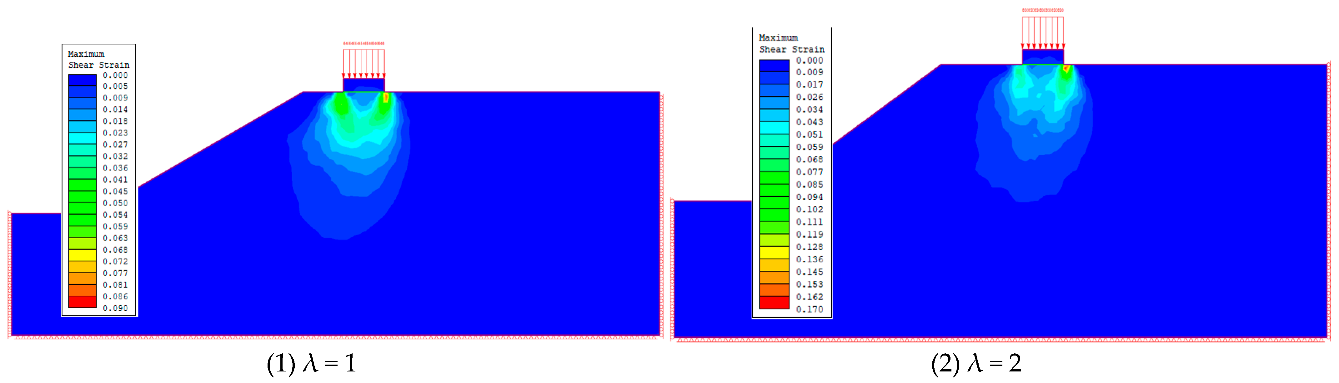
2.1. Finite Element Modeling

The finite element software Phase2D (The software version is phase2D v.8.0.) is used to simulate the damaged state of the slope under different control parameters of the pro-slope characteristics when the foundation above the slope is subjected to maximum load. The foundations near the slopes are schematically shown in Figure 1.

Phase2D (The software version is phase2D v.8.0.), as a professional software integrating elastic–plastic finite element analysis and slope stability assessment, its application in the limit equilibrium method is mainly reflected in the combination with the finite element strength discount method, interactive verification of the model and optimization of engineering practice. The calculation method is to automatically calculate the slope safety coefficient through the finite element strength reduction method, which is based on the principle of gradually reducing the cohesion (c) and the angle of internal friction (φ) of the soil body until the slope reaches the critical damage state. It is found that the FSS obtained by the strength reduction method based on the Mohr-Coulomb model is consistent with the results of the traditional limit equilibrium, which verifies the complementary nature of the two methods.

The construction of a numerical model usually follows two typical paths: the creation of geometric contour is usually completed by CAD platform, designers draw 2D topology through polyline tools, the geometric entity needs to be defined in layers, the internal structure of the surface and the peripheral boundaries of the classification to an independent layer, and ultimately exported to the exchange of DXF format files for subsequent analysis. In the software, the boundary conditions are mainly of three types: symmetric constraints, free constraints and fixed constraints, and the influence of different friction levels on the foundation ground is not considered when establishing the model, i.e., the contact surface between the foundation and the soil is completely smooth, and the red arrow above the foundation in Figure 2 indicates the applied vertical uniform load. The layout of equilateral kneeling nodes adopted by the software has four levels of node distribution density: extra-fine density, fine density, medium density and coarse density, which meets the requirements of different calculation accuracy. According to the literature [28], it is shown that the fine density node distribution can satisfy the computational accuracy requirement of this paper, which is represented as the green part on Figure 2.

The experimental program shown in the

Table 1. Parameters of the foundation soil on the slope.

Parameter Name	Capacity γ/(kN∙m−3)	Modulus of Elasticity E/(kpa)	Poisson’s Ratio	Tensile Strength σt/(kpa)	Angle of Internal Friction φ/(°)	Cohesive Force c/(kpa)
Numerical value	19	50,000	0.38	5	15	50

was designed using the soil quality in the southwest region of China as the basic soil parameter. Step-by-step loading simulation analysis was performed using Phase2D software to discuss the horizontal distance from the foundation to the slope and the slope angle, two characteristic variables on the deformation of the foundation near the slope.

2.2. Finite Element Model Test

The scheme was tested using the control variable method, where the two dependent variables were set as λ and η (where λ denotes the distance from the slope to the foundation as a multiple of the width of the foundation, and η denotes the angle of the slope concerning the level). The test scheme is shown in

Table 2. Phase2D numerical simulation test scheme.

Considerations	Numerical Value
λ	1	1	1	1	2	2	2	2	3	3	3	3
η/(°)	30	45	60	75	30	45	60	75	30	45	60	75

below. The model with λ = 1, η = 45°, in the extracted test is shown in Figure 2.

As can be seen from Figure 3, Figure 4, Figure 5, Figure 6 and Figure 7, when the distance from the slope to the foundation is constant, the ultimate bearing capacity of the foundation decreases with the increase in the slope angle; when the slope angle is constant, the ultimate bearing capacity of the foundation increases with the increase in the distance from the slope to the foundation. In the literature [31], the authors discussed several parameters to replace the depth of the sand layer and the position of the foot of the slope relative to the top of the slope according to the model test, and carried out a series of finite element analyses to validate the results, which showed that the slope angle and the distance from the top of the slope together affect the ultimate bearing capacity and deformation of the foundation, and this comparison verifies the necessity of studying the two controlling factors, namely, the slope angle and the distance from the top of the slope.

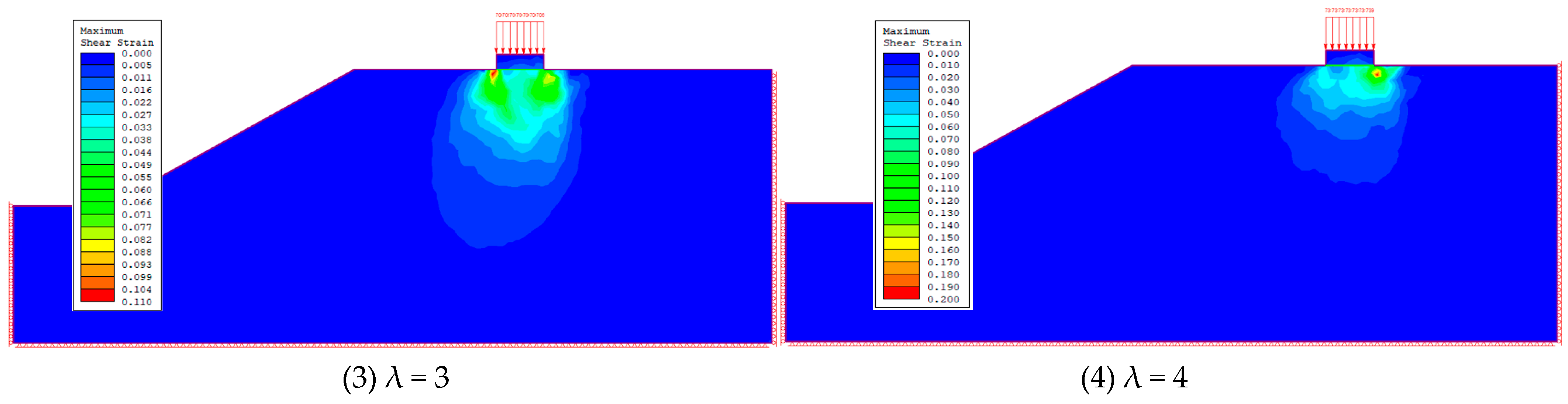
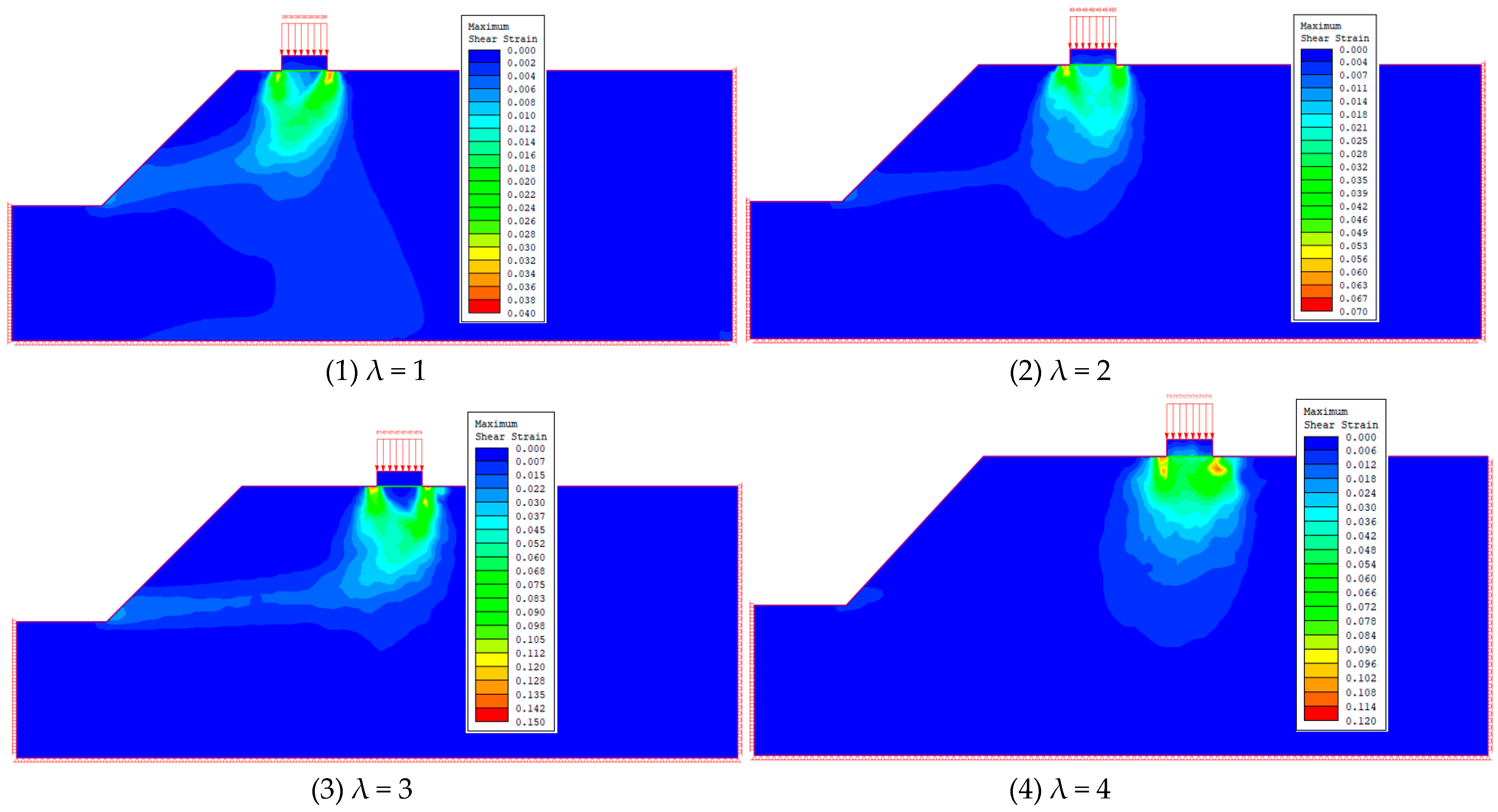
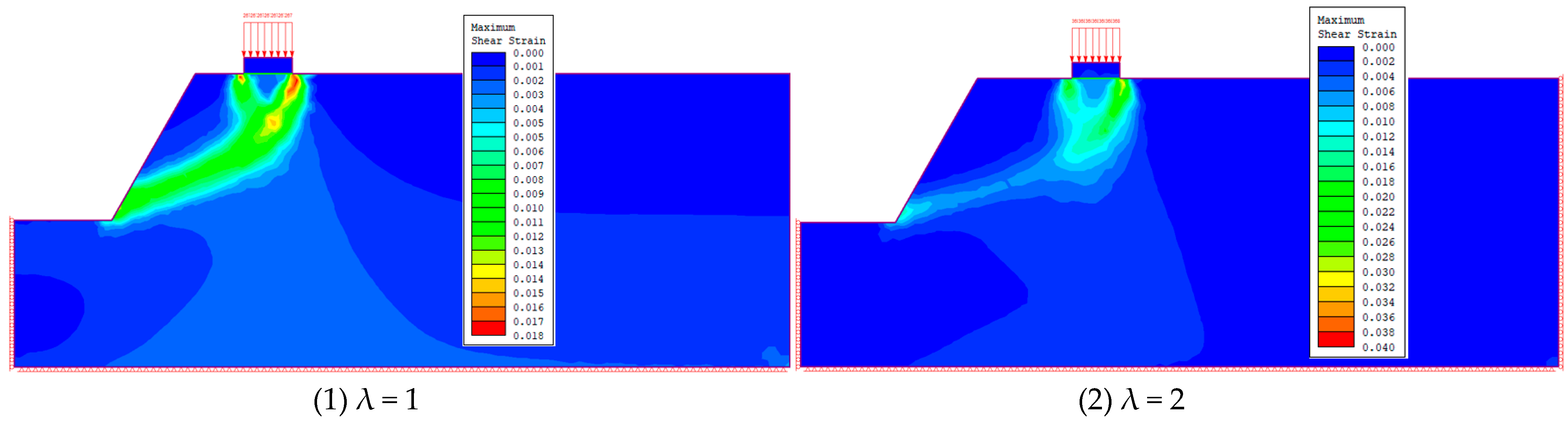
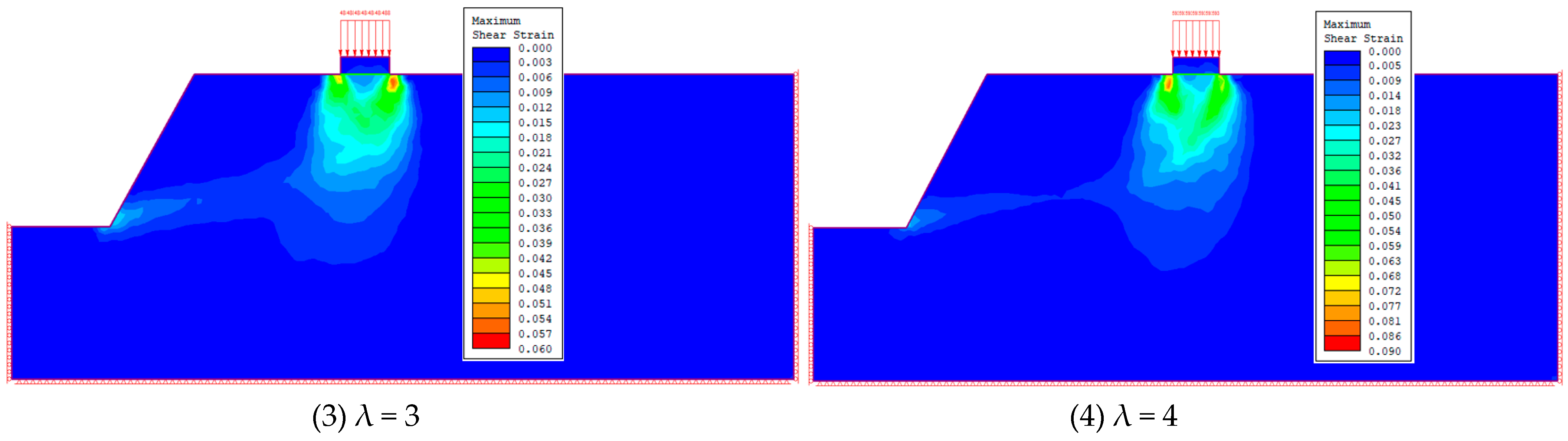
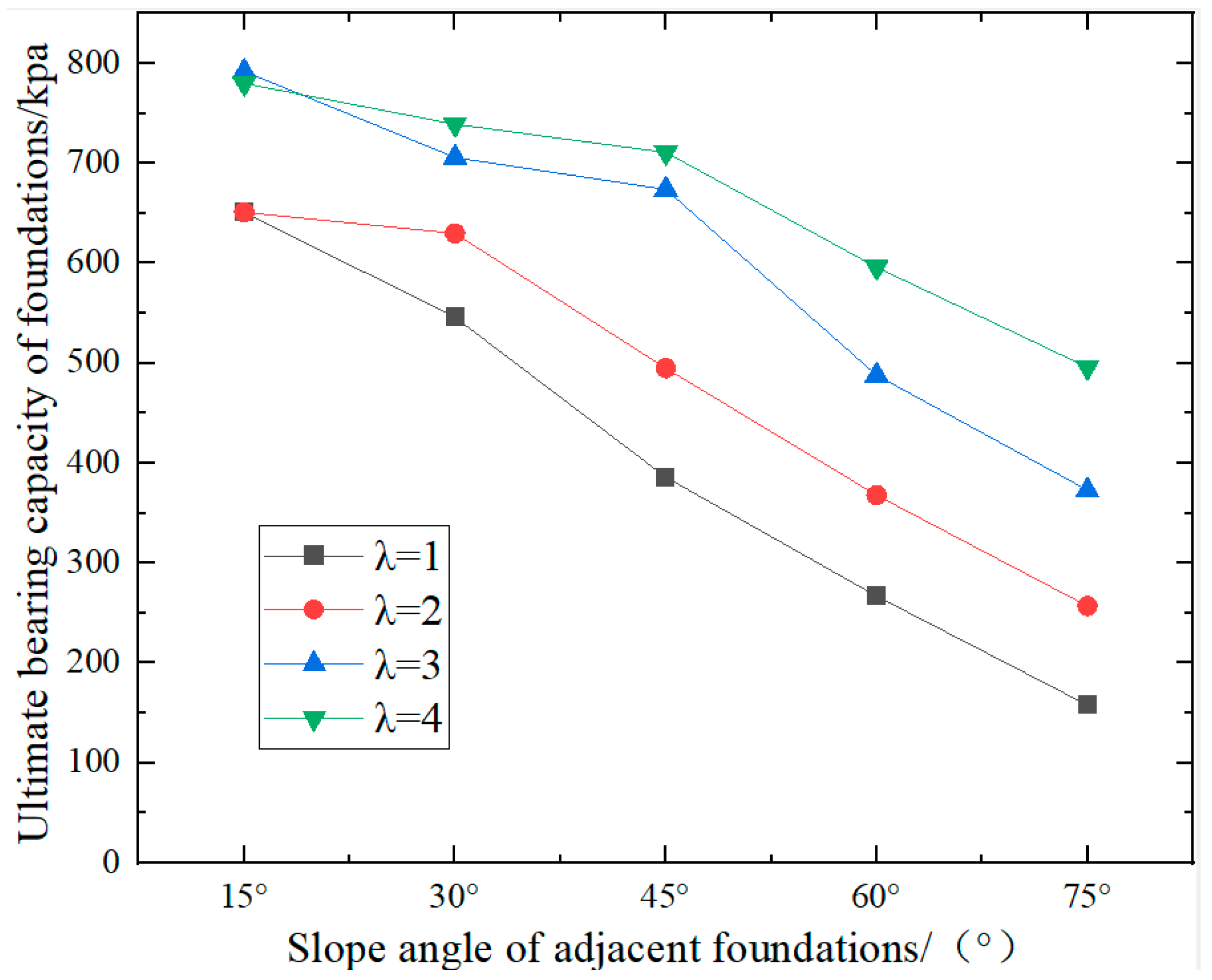
2.3. Analysis of Test Results

Based on the above test, it is evident that the slope angle affects the foundation near the slope: the maximum bearing capacity of the upper part of the strip foundation decreases significantly as the side slope angle increases. At the same time, when the distance from the foundation to the slope increases, the slope angle’s influence on the foundation’s bearing capacity is smaller. The maximum bearing capacity of the foundation when λ ≧ 9 and η ≧ 75° is comparable with that when λ = 0 and β = 15°. This indicates that if the distance from the foundation to the slope is large enough, the effect of the slope angle on the maximum bearing capacity of the foundation can be considered minimal, and at this point, it can be approximated to a horizontal foundation. This is similar to the conclusions obtained in the literature [33] in the experiments. The main reason for this is that the distance from the top of the slope is relatively small. The soil damage zone below the strip foundation is asymmetric, with most of the stress concentrated toward the side of the strip foundation. The damage is mainly shifted to the slope side, so the presence of the slope side has a significant effect on the bearing capacity of the slope foundations. The top of the broken distance is significant, and the foundation of the two sides of the soil damage zone is nearly symmetric.

As shown in Figure 8, under the influence of different foundation-to-slope distances and different slope feet, it can be seen that the foundation-to-slope distance has a more significant influence on the maximum bearing capacity of the adjacent slope foundations. Assuming we obtain the foundation-to-slope distance as the main influence of the formation of different foundation bearing capacity formulae, we can effectively analyze the stability of the foundation near the slope and provide a scientific basis for calculating the bearing capacity of the foundation.

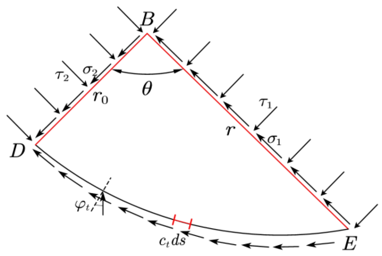
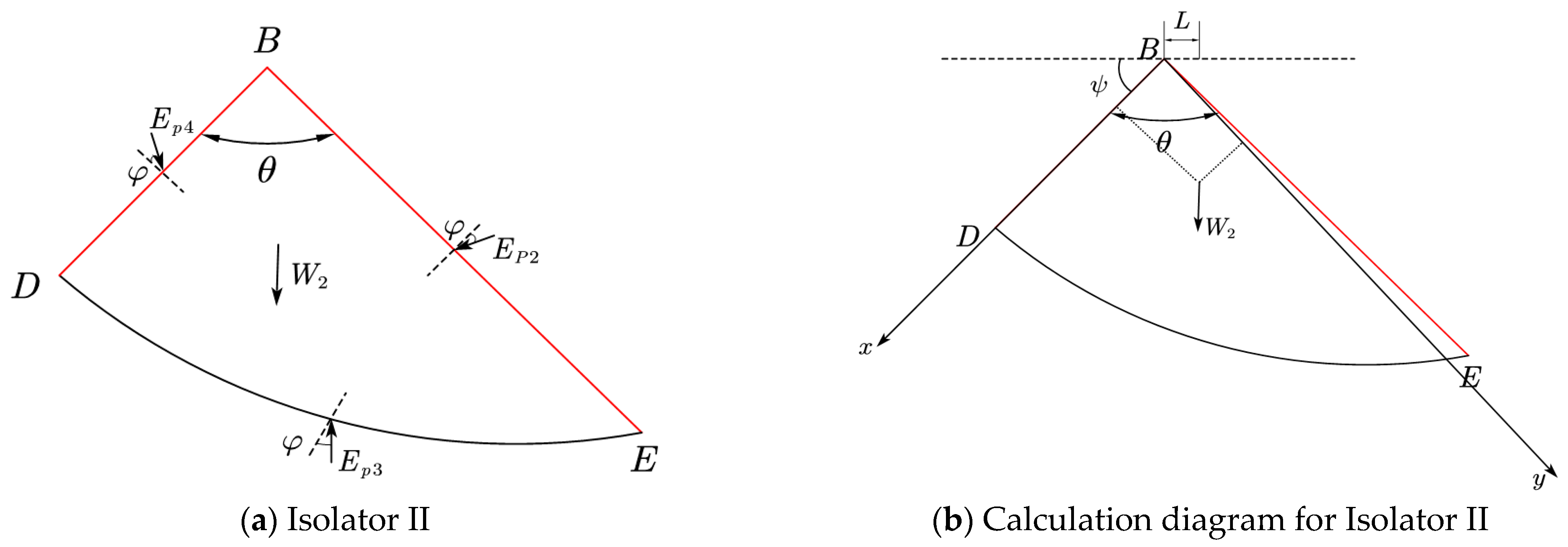
3. Formula Derivation

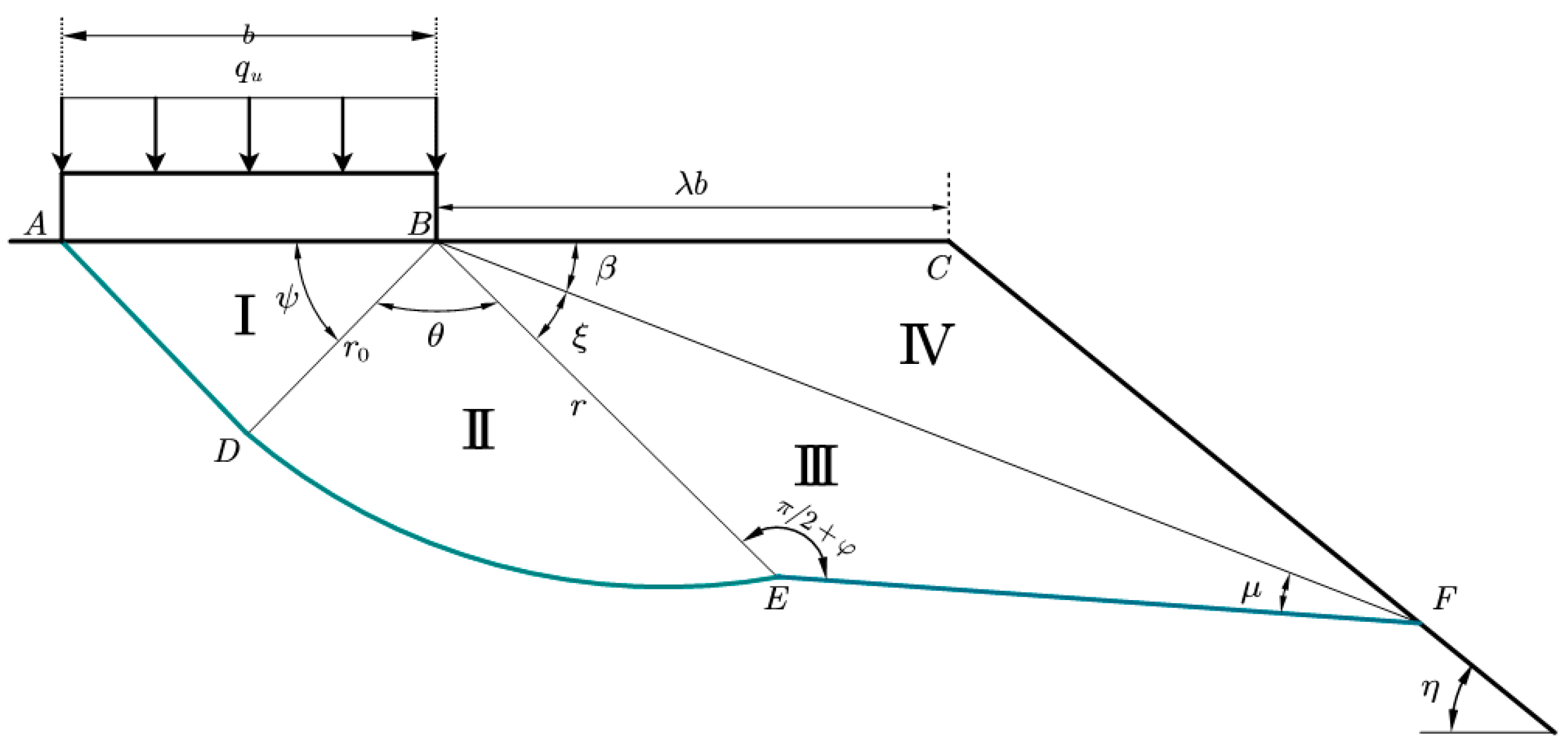
3.1. Basic Assumptions

Figure 9 illustrates a strip foundation of width b located near a slope with an angle of η. The top surface of the slope is horizontal. The top surface of the slope is horizontal, and the horizontal distance from the foundation to the shoulder is λb, where λ represents the ratio of the horizontal distance from the foundation to the shoulder to the width of the foundation. When the foundation soil reaches the maximum bearing capacity qu, the damage mode of the horizontal distance from the foundation to the shoulder is shown in the figure. The damage pattern of the horizontal distance from the foundation to the shoulder is divided into four regions and the following assumptions are made.

(1) The foundation occurs in the overall shear damage mode. The soil on the slip surface is in the plastic limit equilibrium state and satisfies the uniform solution equation of shear strength. The angle between that and the surface is ψ. When the base is completely rough, ψ = φ; when the base is completely smooth, ψ = π/4 + φ/2.

(2) The side adjacent to the slope is damaged first, and it is assumed that the soil destroys the same sliding surface on both sides of the foundation, i.e., area I (ABD) is a symmetric triangular elastic wedge, area II (BDE) is a transitional shear zone, and the DE surface is a logarithmic helix.

(3) Region III (BEF) is a passive damage zone, in which the BE face intersects the slope surface CF at point F. EF is the tangent to the logarithmic helix DE at point E, and the angle between the BE face and EF is π/2 + φ.

(4) Area IV (BCF) is the loosening area, and the BE face is regarded as the equivalent free surface, and the influence of the self-weight W₄ of area IV is reflected by the equivalent stresses (normal stress σ₀ and tangential stress τ₀) on this face.

This section is divided into subheadings, providing a concise and precise description of the experimental results, their interpretation, and the experimental conclusions that can be drawn.

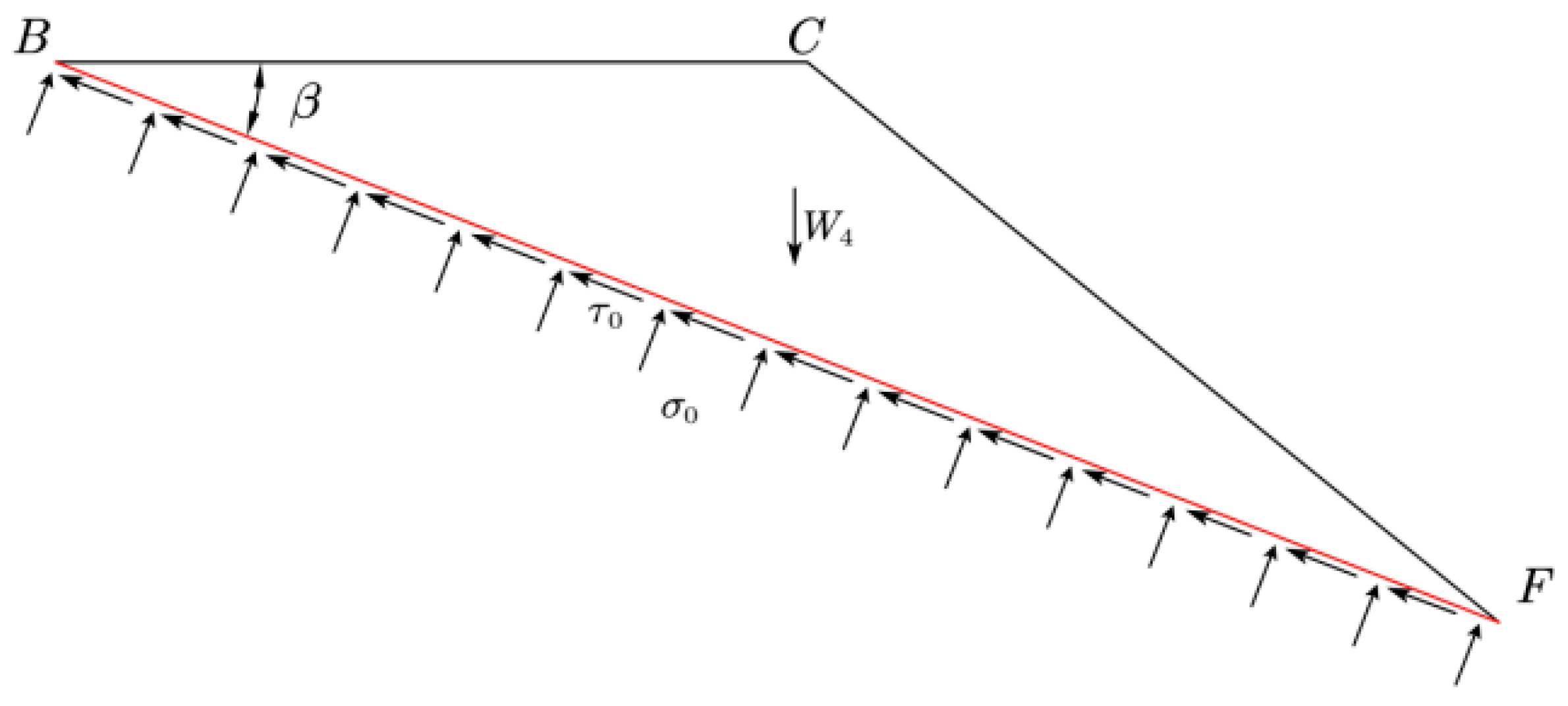
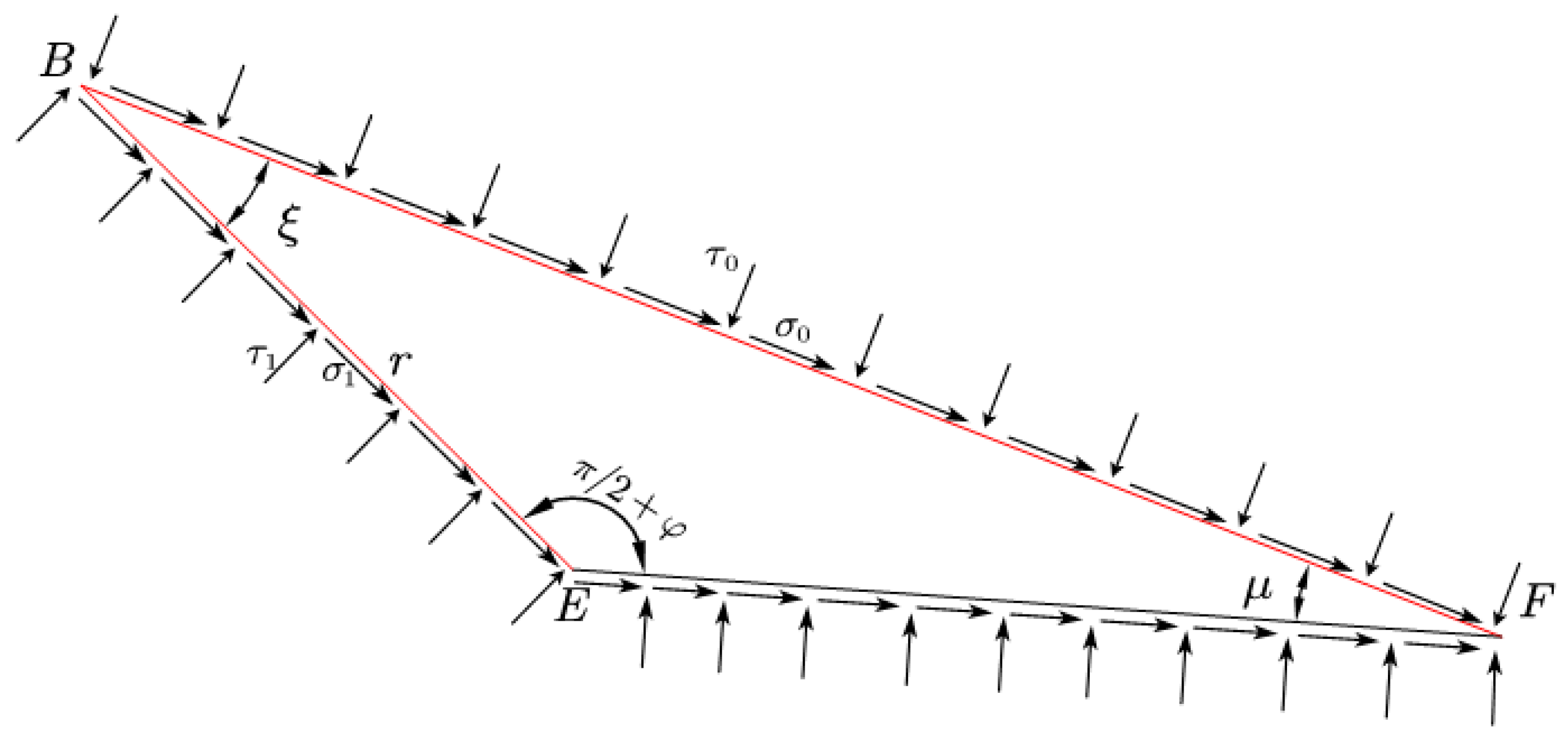
3.2. Deriving a Solution to the Isolation Body Bearing Capacity Equation

Assuming that the foundation soil is gravity-free, the bearing capacity due to cohesion and gravity can be found in the BCF region when γ = 0. qu1. Region IV (BCF) is shown in Figure 10, the arrows on the perpendicular BF plane indicate positive stresses, and the arrows in the direction parallel to the BF plane indicate shear stresses, and the balance of forces in the direction normal to and tangent to the surface of BE is as follows:

$$\overline{BF}{\sigma }_0=W_4\cos \beta$$

(1)

$$\overline{BF}{\tau }_0=W_4\sin \beta$$

(2)

where τ₀ is the tangential stress on the BF surface; σ₀ is the normal stress on the BF surface; W₄ is the self-weight of region IV; β is the angle between the BF surface and the horizontal plane, β ≥ 0; BF is the length of the BF surface; and S₄ is the area of the quadrilateral BCF.

$$W_4=\gamma S_4$$

(3)

$$S_4={\displaystyle \frac{1}{2}}\lambda b{\displaystyle \frac{\lambda b\sin \beta }{\sin \left(\eta -\beta \right)}}\sin \eta$$

(4)

$$\overline{BF}={\displaystyle \frac{\lambda b\sin \eta }{\sin \left(\eta -\beta \right)}}$$

(5)

Substituting Equations (3)–(5) into Equations (1) and (2), the normal stress σ₀ and tangential stress τ₀ on the BE surface are obtained, respectively, as follows:

$${\sigma }_0={\displaystyle \frac{1}{2}}\gamma \lambda \mathrm{bsin}\beta \cos \beta$$

(6)

$${\tau }_0={\displaystyle \frac{1}{2}}\gamma \lambda \mathrm{bsin}\beta \sin \beta$$

(7)

The soil on the BE surface is in plastic limit equilibrium with normal stress σ1 and tangential stress τ₁. Figure 11 shows Mohr’s stress circle, where σ₁ and τ₁ on the BE surface correspond to point e; point f represents σ₀ and τ₀ on the BF surface, and a straight line with the angle of β to the horizontal plane is drawn from the point f to intersect with the Mohr stress circle at point g. The angle between eg and fg is ∠egf = ζ, which is equal to ∠EBF in Figure 12, because the center angle is twice the corresponding circumference angle, so ∠edf = ∠EBF. Then, the angle ∠egf between eg and fg is ζ, which is equal to ∠EBF in Figure 3. Since the angle of the center of the circle is twice the angle of the corresponding circumference, ∠edf = 2ζ.

According to the law of sines of triangle BDE, we have

$${\displaystyle \frac{\overline{BF}}{\sin (\frac{\pi }{2}+\phi )}}={\displaystyle \frac{\overline{BE}}{\sin (\mu )}}={\displaystyle \frac{\overline{BE}}{\sin (\frac{\pi }{2}-\phi -\xi )}}$$

(8)

where the length of BE and DE is the logarithmic helix and the length of the BE surface is

$$\overline{BD}={\displaystyle \frac{\mathrm{b}}{2\cos \psi }}$$

(9)

$$\overline{BE}=\overline{BD}{\mathrm{e}}^{\theta \tan \phi }={\displaystyle \frac{{\mathrm{be}}^{\theta \tan \phi }}{2\cos \psi }}$$

(10)

The θ angle can be recognized by the geometrical relation:

$$\theta =\pi -\psi -\beta -\xi$$

(11)

The above equation embodies the relationship between β and ζ, φ, ψ, η, λ, and b. The trial algorithm is used to solve for the value of the angle β. The specific process is as follows: Firstly, assume a value of β, and then calculate σ₀ and τ₀ according to Equations (6) and (7). Then, through the geometric relationship in the figure, find the angle ζ between the BE surface and the BF surface. Then, according to the calculation of Equation (10), obtain the value of θ and then substitute the values of ζ and θ into Equation (13) to obtain the calculated value of β. Repeat this iterative process until the difference between the assumed and calculated values of β meets the accuracy requirements.

Organized form:

$${\displaystyle \frac{\frac{\lambda b\sin \eta }{\sin \left(\eta -\beta \right)}}{\sin (\frac{\pi }{2}+\phi )}}={\displaystyle \frac{\frac{{\mathrm{be}}^{\theta \tan \phi }}{2\cos \psi }}{\sin (\frac{\pi }{2}-\phi -\xi )}}$$

(12)

Derived form:

$$\sin \left(\eta -\beta \right)={\displaystyle \frac{\lambda b\sin \eta \sin (\frac{\pi }{2}-\phi -\xi )2\cos \psi }{{\mathrm{be}}^{\theta \tan \phi }\sin (\frac{\pi }{2}+\phi )}}$$

(13)

The corresponding τ₀ and τ₁ values can be obtained through the geometric relation as follows:

$$\overline{\mathrm{df}}={\displaystyle \frac{{\tau }_0}{\cos (2\xi +\phi )}}={\displaystyle \frac{{\tau }_1}{\cos \phi }}=\overline{\mathrm{de}}$$

(14)

Then, there is

$${\tau }_1={\displaystyle \frac{{\tau }_0\cos \phi }{\cos (2\xi +\phi )}}$$

(15)

$${\sigma }_1={\sigma }_0+{\displaystyle \frac{{\tau }_1}{\cos \phi }}[\sin (2\xi +\phi )-\sin \phi ]$$

(16)

Substituting τ₁ = c_t + σ_ttanφ into (16), σ₁ can be organized as follows:

$${\sigma }_1={\sigma }_0+{\displaystyle \frac{{\tau }_0[\sin (2\xi +\phi )-\sin \phi ]}{\cos (2\xi +\phi )}}$$

(17)

As shown in Figure 13, the arrows pointing perpendicularly to region II are positive stresses and the arrows in the parallel direction are tangential stresses. From the balance of moments at point B, we obtain

$${\displaystyle \sum M_{\mathrm{B}}}={\displaystyle \frac{1}{2}}{\sigma }_1{\overline{BE}}^2-{\displaystyle \frac{1}{2}}{\sigma }_2{\overline{BD}}^2+{\displaystyle {\int }_0^{\theta }{\mathrm{c}}_{\mathrm{t}}}{\mathrm{r}}^2\mathrm{d}\theta =0$$

(18)

$${\displaystyle {\int }_0^{\theta }{\mathrm{c}}_{\mathrm{t}}}{\mathrm{r}}^2\mathrm{d}\theta ={\displaystyle \frac{{\mathrm{c}}_{\mathrm{t}}{\overline{BD}}^2}{2\tan \phi }}(e^{2\theta \tan \phi }-1)$$

(19)

Substituting Equation (19) into Equation (18) gives

$${\sigma }_2=[{\mathrm{c}}_{\mathrm{t}}(e^{2\theta \tan \phi }-1)+({\displaystyle \frac{1}{2}}\gamma \lambda \mathrm{bsin}\beta \cos \beta +{\displaystyle \frac{\gamma \lambda {\mathrm{bsin}}^2\beta \sin (2\xi +\phi )}{2\cos (2\xi +\phi )}}-{\displaystyle \frac{\gamma \lambda {\mathrm{bsin}}^2\beta \sin \phi }{2\cos \left(2\xi +\phi \right)}}){\mathrm{e}}^{2\theta \tan \phi }\tan \phi ]\cot \phi$$

(20)

$${\tau }_2={\mathrm{c}}_{\mathrm{t}}+{\sigma }_2\tan \phi =({\mathrm{c}}_{\mathrm{t}}+{\sigma }_1\tan \phi ){\mathrm{e}}^{2\theta \tan \phi }$$

(21)

Organized form:

$${\tau }_2=[{\mathrm{c}}_{\mathrm{t}}+({\displaystyle \frac{1}{2}}\gamma \lambda \mathrm{bsin}\beta \cos \beta +{\displaystyle \frac{\gamma \lambda {\mathrm{bsin}}^2\beta [\sin (2\xi +\phi )-\sin \phi ]}{2\cos (2\xi +\phi )}})\tan \phi ]{\mathrm{e}}^{2\theta \tan \phi }$$

(22)

As shown in Figure 14, the arrows pointing perpendicularly to region I are positive stresses and the arrows in the parallel direction are tangential stresses, and arrows above the AB surface indicate the load carrying capacity sought in this paper. Take the isolate I, in which the force balance in the vertical direction is

$$q_{u1}-{\displaystyle \frac{{\sigma }_2}{\cos \psi }}\cos \psi -{\displaystyle \frac{{\tau }_2}{\cos \psi }}\sin \psi =0$$

(23)

Organized form:

$$q_{u1}={\sigma }_2+{\tau }_2\tan \psi$$

(24)

To solve the bearing capacity caused by soil self-weight q_u2, it is assumed that c = 0 and σ₀ = τ₀ = 0. Since the self-weight of soil in region IV has been taken into account in the derivation of q_u1, the derivation of q_u2 starts from region III. The force analysis of isolator III is shown in Figure 15. The force equilibrium of isolator III in horizontal and vertical directions is obtained.

By balancing the forces on BD,

$$W_3=\gamma S_3$$

(25)

$$W_3\sin \epsilon -E_{\mathrm{p}2}\cos \phi =0$$

(26)

via the BDE sine theorem:

$${\displaystyle \frac{\overline{BE}}{\sin \mu }}={\displaystyle \frac{\overline{BF}}{\sin \left(\frac{\pi }{2}+\phi \right)}}$$

(27)

This is obtained by substituting Equation (5) into Equation (27) as follows:

$$\overline{BE}={\displaystyle \frac{\overline{BE}}{\sin \left(\frac{\pi }{2}+\phi \right)}}\sin \mu ={\displaystyle \frac{\lambda \mathrm{bsin}\eta \sin \mu }{\sin \left(\frac{\pi }{2}+\phi \right)\sin \left(\eta -\beta \right)}}$$

(28)

Among them,

$$S_3={\displaystyle \frac{1}{2}}\overline{BE}\overline{BF}\sin \xi ={\displaystyle \frac{{\lambda }^2{\mathrm{b}}^2{\sin }^2\eta \sin \mu \sin \xi }{2\sin \left(\frac{\pi }{2}+\phi \right){\sin }^2\left(\eta -\beta \right)}}$$

(29)

$$W_3=\gamma S_3={\displaystyle \frac{\gamma {\lambda }^2{\mathrm{b}}^2{\sin }^2\eta \sin \mu \sin \xi }{2\sin \left(\frac{\pi }{2}+\phi \right){ \sin }^2\left(\eta -\beta \right)}}$$

(30)

$$E_{\mathrm{p}2}={\displaystyle \frac{W_3\sin \epsilon }{\cos \phi }}={\displaystyle \frac{\gamma {\lambda }^2{\mathrm{b}}^2{\sin }^2\eta \sin \mu \sin \xi \sin \epsilon }{2\sin \left(\frac{\pi }{2}+\phi \right){ \sin }^2\left(\eta -\beta \right) \cos \phi }}$$

(31)

As shown in Figure 16a, the force analysis of isolation body II considers the self-weight of the soil, where Ep4 represents the combined force of the counterforce on the BD face. This produces an angle of φ with the normal direction of the BD face and acts at a distance of BD/2 from point D. W2 is the self-weight of the soil of the isolation body II, which acts at the center of gravity. E_p3 is the radial force on the DE face considering the self-weight of the soil, which produces an angle of φ with the normal direction of the DE face, in which the line of action passes through point B. From the equilibrium of moments at point B, we have

$${\displaystyle \frac{1}{2}}\cdot {\displaystyle \frac{\mathrm{b}}{2\cos \psi }}{E}_{p4}\cos \phi ={\displaystyle \frac{1}{2}}\overline{BD}{E}_{p2}\cos \phi +L{W}_2$$

(32)

Further,

$$E_{p4}={\displaystyle \frac{2\left(\overline{BD}{E}_{p2}\cos \phi +2L{W}_2\right)\cos \psi }{\mathrm{b}\cos \phi }}$$

(33)

Among them,

$$W_2=\gamma S_2$$

(34)

$$S_2={\displaystyle \frac{{\overline{BD}}^2\left(e^{2\theta \tan \phi }-1\right)}{4\tan \phi }}$$

(35)

$$\overline{BD}={\displaystyle \frac{\mathrm{b}}{2\cos \psi }}$$

(36)

As shown in Figure 16b, the action point of W₂ is located at the center of the shape of the isolate BED to determine the location of the center of the shape of the BED. The B point is considered the origin, and the BD represents the x-axis to establish a right-angle coordinate system, as shown in the figure. Because ED is a logarithmic helix, the coordinates of the center of the fan BED form O are

$$x_1={\displaystyle \frac{4\tan \phi \left[e^{3\theta \tan \phi }\left(\sin \theta +3\tan \phi \cos \theta \right)-3\tan \phi \right]}{3\left(1+9{\tan }^2\phi \right)\left(e^{2\theta \tan \phi }-1\right)}}\overline{BD}$$

(37)

$${\mathrm{y}}_1={\displaystyle \frac{4\tan \phi \left[e^{3\theta \tan \phi }\left(3\tan \phi \cos \theta -\cos \theta \right)+1\right]}{3\left(1+9{\tan }^2\phi \right)\left(e^{2\theta \tan \phi }-1\right)}}\overline{BD}$$

(38)

The horizontal distance L from W2 to point B is

$$L={\mathrm{y}}_1\sin \psi -x_1\cos \psi$$

(39)

By substituting Equations (37) and (38) into Equation (39), the following is obtained:

$$L={\displaystyle \frac{2\mathrm{btan}\psi \tan \phi \left[e^{3\theta \tan \phi }\left(3\tan \phi \cos \theta -\cos \theta \right)+1\right]}{3\left(1+9{\tan }^2\phi \right)\left(e^{2\theta \tan \phi }-1\right)}}-{\displaystyle \frac{2\mathrm{b}\tan \phi \left[e^{3\theta \tan \phi }\left(\sin \theta +3\tan \phi \cos \theta \right)-3\tan \phi \right]}{3\left(1+9{\tan }^2\phi \right)\left(e^{2\theta \tan \phi }-1\right)}}$$

(40)

Force analysis of isolate I considering the weight of the soil:

As shown in Figure 17, among them,

$$W_1=\gamma S_1$$

(41)

$$S_1={\displaystyle \frac{1}{2}}{b}^2\tan \psi$$

(42)

Substituting Equation (42) into Equation (41) yields

$$W_1={\displaystyle \frac{1}{2}}\gamma b^2\tan \psi$$

(43)

From the vertical force equilibrium, the bearing capacity provided by the self-weight of the soil body q_u2 is given by

$${\mathrm{q}}_{\mathrm{u}2}\mathrm{b}+{\mathrm{W}}_1=2E_{\mathrm{p}4}\cos \phi \cos \psi$$

(44)

Substituting Equation (43) into Equation (44) gives

$${\mathrm{q}}_{\mathrm{u}2}={\displaystyle \frac{2E_{\mathrm{p}4}\cos \phi \cos \psi -\frac{1}{2}\gamma b^2\tan \psi }{\mathrm{b}}}$$

(45)

The superimposed bearing capacities q_u1 and q_u2, i.e., Equations (24) and (45), yield the ultimate bearing capacity under the horizontal distance from the foundation to the shoulder q_u as follows:

$$\begin{array}{ll}\hfill \mathrm{qu}& =\mathrm{qu}1+\mathrm{qu}2\\ & ={\mathrm{t}}_{\mathrm{c}}[(e^{2\theta \tan \phi }-1)\cot \phi +{\mathrm{e}}^{2\theta \tan \phi }\tan \psi +{\displaystyle \frac{{\mathrm{e}}^{2\theta \tan \phi }[\sin (2\xi +\phi )-\sin \phi ]}{\cos \phi -\tan \phi [\sin (2\xi +\phi )-\sin \phi ]}}\\ & +{\displaystyle \frac{\tan \phi {\mathrm{e}}^{2\theta \tan \phi }\tan \psi [\sin (2\xi +\phi )-\sin \phi ]}{\cos \phi -\tan \phi [\sin (2\xi +\phi )-\sin \phi }}]+{\sigma }_0{\displaystyle \frac{{[\mathrm{e}}^{2\theta \tan \phi }+\tan \phi {\mathrm{e}}^{2\theta \tan \phi }\tan \psi ]\cos \phi }{\cos \phi -\tan \phi [\sin (2\xi +\phi )-\sin \phi ]}}+{\displaystyle \frac{2E_{\mathrm{p}4}\cos \phi \cos \psi -\frac{1}{2}\gamma b^2\tan \psi }{\mathrm{b}}}\end{array}$$

(46)

In summary, the limit equilibrium method can successfully derive the relationship between the ultimate bearing capacity q_u of a slope-facing foundation and its slope-facing distance. However, the application of this formula has certain limitations: (1) the foundation material must be single, homogeneous, and must not contain weak interlayers or undergo significant deformation; (2) the surface of the top of the slope must be flat, with no significant changes in the slope; and (3) the foundation must have a shallow depth of burial and be categorized as a shallow foundation. Therefore, an important direction for future research is to develop a formula for calculating the ultimate bearing capacity of a pro-slope foundation that can synthesize multiple factors. Nonetheless, the formula has a fairly wide range of applications for numerous engineering construction projects and can provide theoretical support and reference for engineering practice.

4. Application Examples and Comparative Validation

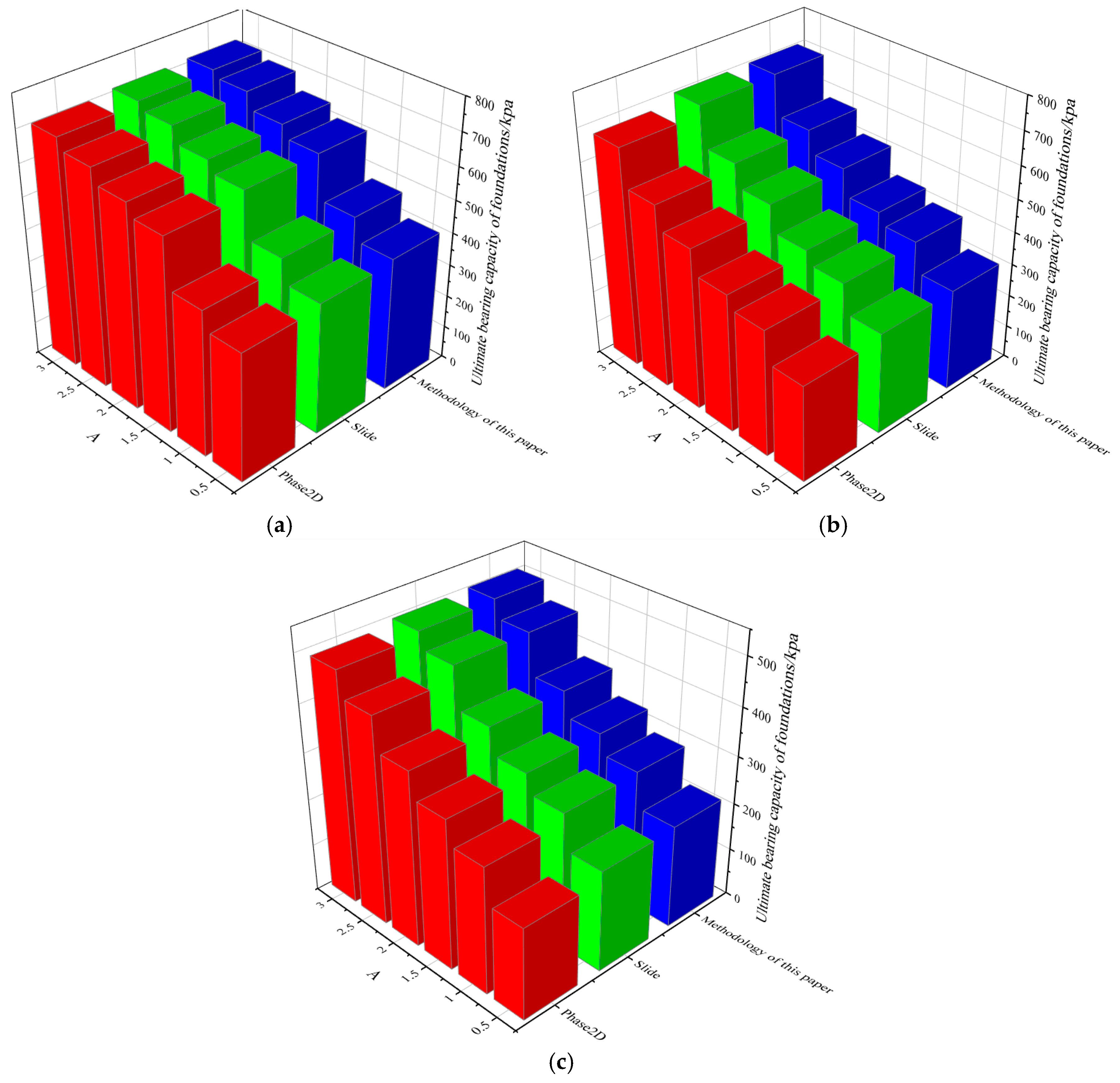
We established an analytical model for the ultimate bearing capacity of pro-slope strip foundations using the rigid-body limit equilibrium analysis method and its optimized solution approach. In order to verify the rationality and feasibility of the model, we analyzed it via specific examples and numerical simulations, discussing it in depth along with the limit ring method. Finally, the calculation results were analyzed and discussed in detail.

4.1. Case Studies

A slope-facing strip foundation with a width of b = 3 m and soil properties that include a foundation soil cohesion of c = 10 KPa, an internal friction angle of φ = 30°, a foundation soil gravity of γ = 18 KN/m, and side slope angles (β) of 30°, 45°, and 60° was calculated. Comparisons were made using the methods of this paper as well as those from the literature, with the results of the analysis shown in Figure 18.

By comparing the results of this research method with other methods in specific cases, we can draw the following conclusions:

(1) There are differences in the computational results of the ultimate bearing capacity of foundations on adjacent slopes, as obtained by the three different computational methods. These differences are mainly due to their respective theoretical bases and underlying assumptions. Nevertheless, these results are quite close, and our results lie exactly between those of the other two methods, showing better stability for engineering applications. This demonstrates the validity and rationality of the methodology used in this study.

(2) Unlike the studies [32,33], which mainly focus on calculating the bearing capacity of slope-facing foundations, the method used in this study not only accurately calculates the bearing capacity of slope-facing foundations but also introduces the concept of slope-facing distance, which results in the calculation results being closer to those of actual engineering cases. This further proves the applicability and rationality of the method used in this study.

4.2. Comparative Numerical Analysis

The software Phase2D and Slide (The software version is slidev 0.10.2) were used to calculate the ultimate bearing capacity of the foundations on the critical slopes, which were then compared to the calculation method proposed in this paper. In this process, two cases with slope angle η values of 30°, 45°, and 60° were selected based on the soil parameters listed in the table. A series of calculations were carried out for different pro-slope distances, i.e., 0.5, 1, 1.5, 2, 2.5, and 3.

Based on the comparison of data in Figure 19, it can be seen that there are certain differences between the results of this study and those of the numerical simulations. These differences may be due to factors such as model construction, parameter selection, and mesh division in the numerical simulation process, as well as the limitations of the underlying assumptions and reference factors of the formulas. Despite these differences, the computational results of this study still show good agreement with those of the numerical simulations and more closely align with the analytical results from the Slide software. The Slide software uses the limit equilibrium method to derive the results by analyzing the force transfer of the slide, which is similar to the computational method used in this study, further confirming the accuracy and applicability of this study’s methodology. The analysis results show that the obtained results are closer to the real solution of the ultimate bearing capacity of foundations near slopes. The results can better reflect the actual ultimate bearing capacity of foundations near slopes and have certain theoretical significance for the optimal design of foundations near slopes.

5. Conclusions

This paper investigates the ultimate bearing capacity of shallow foundations situated on slopes by considering various factors, employing the finite element software Phase2D, and constructing a planar model of slope foundations. It evaluates the ultimate bearing capacity of shallow foundations about different slope distances, derives a calculation formula for the correlation between ultimate bearing capacity and the distance from the top of the slope, and compares it with similar studies from the literature and cases. The main conclusions obtained are as follows.

1. Compared with other theoretical calculation methods, this study uses the limit equilibrium method and constructs a new calculation model, which incorporates the distance factor from the foundation to the slope when calculating the ultimate bearing capacity of slope-facing foundations, so that the calculated ultimate bearing capacity is closer to engineering practice and more widely applicable.

2. By comparing and analyzing the engineering examples with the existing research results and numerical simulation results, the calculation results obtained in this paper are highly consistent with the existing research and numerical simulation results, and are closer to the results obtained by using the same theoretical calculation method, which confirms the accuracy of the method in this paper.

In order to make the results of the theoretical calculations in this paper and the theoretical calculated results closer, but also at the same time to prove the accuracy of this method. The asymmetric model was chosen to investigate the ultimate bearing capacity of the slope foundation, this choice, did not take into account the influence of the legend on the left side of the foundation for the slope foundation, this negligence also led to the results of the calculation of a certain deviation but does not affect the overall results of the calculation. In addition, since the model does not take into account the deformation characteristics of the foundation material, it may lead to bearing capacity failure when the actual load is much smaller than the bearing capacity of the foundation, resulting in a high value of the calculated bearing capacity. Future research should further investigate the effect of foundation deformation on the bearing capacity of sloping foundations. Therefore, in order to further consider its accuracy, calculating a formula for calculating the ultimate bearing capacity of slopeside foundations that can take into account the full range of factors is a direction that deserves in-depth exploration and research in the future.

References

1. Shabani, M.J.; Shamsi, M.; Ghanbari, A. Dynamic response of three-dimensional midrise buildings adjacent to slope under seismic excitation in the direction perpendicular to the slope. Int. J. Geomech. ASCE 2021, 21, 04021204. [Google Scholar] [CrossRef]
2. Fatahi, B.; Huang, B.H.; Yeganeh, N.; Terzaghi, S.; Banerjee, S. Three-dimensional simulation of seismic slope-foundation-structure interaction for buildings near shallow slopes. Int. J. Geomech. ASCE 2020, 20, 04019140. [Google Scholar] [CrossRef]
3. Bai, T.; Qiu, T.; Huang, X.; Li, C. Locating global critical slip surface using the Morgenstern-Price method and optimization technique. Int. J. Geomech. 2014, 14, 319–325. [Google Scholar] [CrossRef]
4. Biniyaz, A.; Azmoon, B.; Liu, Z. Coupled transient saturated–unsaturated seepage and limit equilibrium analysis for slopes: Influence of rapid water level changes. Acta Geotech. 2022, 17, 2139–2156. [Google Scholar] [CrossRef]
5. Cai, F.; Ugai, K. Numerical analysis of rainfall effects on slope stability. Int. J. Geomech. 2004, 4, 69–78. [Google Scholar] [CrossRef]
6. Cheng, Y.M. Location of critical failure surface and some further studies on slope stability analysis. Comput. Geotech. 2003, 30, 255–267. [Google Scholar] [CrossRef]
7. Cheng, Y.M.; Lau, C.K. Slope Stability Analysis and Stabilization: New Methods and Insight, 1st ed.; CRC Press: Boca Raton, FL, USA, 2008. [Google Scholar] [CrossRef]
8. Fathipour, H.; Tajani, S.B.; Payan, M.; Chenari, R.J.; Senetakis, K. Impact of transient infiltration on the ultimate bearing capacity of obliquely and eccentrically loaded strip footings on partially saturated soils. Int. J. Geomech. 2023, 23, 1–19. [Google Scholar] [CrossRef]
9. Caramana, E.J. The implementation of slide lines as a combined force and velocity boundary condition. J. Comput. Phys. 2009, 228, 3911–3916. [Google Scholar] [CrossRef]
10. Clair, G.; Després, B.; Labourasse, E. A one-mesh method for the cell-centered discretization of sliding. Comput. Methods Appl. Mech. Eng. 2014, 269, 315–333. [Google Scholar] [CrossRef]
11. Zhu, Y.; Du, J. Sliding Line Point Regression for Shape Robust Scene Text Detection. In Proceedings of the 2018 24th International Conference on Pattern Recognition (ICPR), Beijing, China, 20–24 August 2018; pp. 3735–3740. [Google Scholar] [CrossRef]
12. Roy, A.; Noel, M.M. Design of a high-speed line following robot that smoothly follows tight curves. Comput. Electr. Eng. 2016, 56, 732–747. [Google Scholar] [CrossRef]
13. Zhai, J.; Song, Z. Adaptive sliding mode trajectory tracking control for wheeled mobile robots. Int. J. Control 2018, 92, 2255–2262. [Google Scholar] [CrossRef]
14. Fraldi, M.; Guarracino, F. Evaluation of Impending Collapse in Circular Tunnels by Analytical and Numerical Approaches. Tunn. Undergr. Space Technol. 2011, 26, 507–516. [Google Scholar] [CrossRef]
15. Mollon, G.; Dias, D.; Soubra, A.H. Rotational Failure Mechanisms for the Face Stability Analysis of Tunnels Driven by a Pressurized Shield. Int. J. Numer. Anal. Methods Geomech. 2011, 35, 1363–1388. [Google Scholar] [CrossRef]
16. Wilson, D.; Abbo, A.; Sloan, S. Undrained Stability of a Square Tunnel Where the Shear Strength Increases Linearly with Depth. Comput. Geotech. 2013, 49, 314–325. [Google Scholar] [CrossRef]
17. Yang, X.-L.; Qin, C.-B. Limit Analysis of Rectangular Cavity Subjected to Seepage Forces Based on Hoek-Brown Failure Criterion. Geomech. Eng. 2014, 6, 503–515. Available online: https://api.semanticscholar.org/CorpusID:129222228 (accessed on 24 March 2025).
18. Yang, X.-L.; Yan, R.-M. Collapse Mechanism for Deep Tunnel Subjected to Seepage Force in Layered Soils. Geomech. Eng. 2015, 8, 741–756. [Google Scholar] [CrossRef]
19. Yu, S.B.; Zhang, X.; Sloan, S.W. A 3D upper bound limit analysis using radial point interpolation meshless method and second-order cone programming. Int. J. Numer. Methods Eng. 2016, 108, 1686–1704. [Google Scholar] [CrossRef]
20. Yuan, S.; Du, J.N. Effective stress-based upper bound limit analysis of unsaturated soils using the weak form quadrature element method. Method. Comput. Geotech. 2018, 98, 172–180. [Google Scholar] [CrossRef]
21. Huang, M.S.; Fan, X.P.; Wang, H.R. Three-dimensional upper bound stability analysis of slopes with weak interlayer based on rotational-translational mechanisms. Eng. Geol. 2017, 223, 82–91. [Google Scholar] [CrossRef]
22. Monforte, L.; Arroyo, M.; Carbonell, J.M.; Gens, A. Numerical simulation of undrained insertion problems in geotechnical engineering with the particle finite element method (PFEM). Comput. Geotech. 2017, 82, 144–156. [Google Scholar] [CrossRef]
23. Singh, P.K.; Kumar, M. Hypervelocity impact behavior of projectile penetration on spacecraft structure: A review. Mater. Today Proc. 2022, 62, 67–71. [Google Scholar] [CrossRef]
24. Baazouzi, M.; Benmeddour, D.; Mabrouki, A.; Nouiri, M. 2D numerical analysis of shallow foundation rested near slope under inclined loading. Procedia Eng. 2016, 143, 1234–1241. [Google Scholar] [CrossRef]
25. Kusakabe, O.; Kimura, T.; Yamaguchi, H. Bearing capacity of slopes under strip load on the top surfaces. Soils Found. 1981, 21, 29–35. [Google Scholar] [CrossRef] [PubMed]
26. Yang, X.L.; Wang, Z.B.; Zou, J.F.; Li, L. Bearing capacity of foundation on slope determined by energy dissipation method and model experiments. J. Cent. South Univ. Technol. 2007, 14, 125–128. [Google Scholar] [CrossRef]
27. Yang, X.L.; Guo, N.Z.; Zhao, L.H.; Li, L. Influences of nonassociated flow rules on seismic bearing capacity factors of strip footing on soil slope by energy dissipation method. J. Cent. South Univ. Technol. 2007, 14, 842–847. [Google Scholar] [CrossRef]
28. Yang, S.C.; Leshchinsky, B.; Cui, K.; Zhang, F.; Gao, Y.F. Unified approach toward evaluating bearing capacity of shallow foundations near slopes. J. Geotech. Geoenviron. Eng. 2019, 145, 04019110. [Google Scholar] [CrossRef]
29. Zhao, L.; Luo, Q.; Yang, F. Calculation of upper limit of bearing capacity of slope-facing strip foundation. J. Wuhan Univ. Technol. (Transp. Sci. Eng. Ed.) 2010, 34, 84–87. [Google Scholar]
30. Feng, Y.; Yang, J.; Zhang, X.; Zhao, L. One-side slip failure mechanism and upper bound solution for bearing capacity of foundation on slope. Eng. Mech. 2010, 27, 162–168. [Google Scholar]
31. Casablanca, O.; Biondi, G.; Cascone, E. Static and seismic bearing capacity of shallow strip foundations on slopes. Géotechnique 2022, 72, 769–783. [Google Scholar] [CrossRef]
32. El Sawwaf, M.A. Behavior of strip footing on geogrid-reinforced sand over a soft clay slope. Geotext. Geomembr. 2007, 25, 50–60. [Google Scholar] [CrossRef]
33. El Sawwaf, M.A.; Nazir, A.K. Cyclic settlement behavior of strip footings resting on reinforced layered sand slope. J. Adv. Res. 2012, 3, 315–324. [Google Scholar] [CrossRef]
34. Faghihmaleki, H.; Nazari, H. Laboratory study of metakaolin and microsilica effect on the performance of high-strength concrete containing Forta fibers. Adv. Bridg. Eng. 2023, 4, 11. [Google Scholar] [CrossRef]
35. Bagheri Kalaye, A. The Effect of Non-implementation of the Beam Roof of the Last Floor Block on the Irregularity of the Analysis and Design of the Structure. J. Civ. Asp. Struct. Eng. 2024, 1, 197–204. [Google Scholar]
36. Bararpour, M.; Delfani, M. Tensile and Compressive Strength Investigations of Ordinary Concrete and Pozzolanic Concrete and the Effect of Polypropylene on Them. J. Civ. Asp. Struct. Eng. 2024, 1, 113–120. [Google Scholar]
Figure 1. Geometric model of foundations near slopes.
Buildings 15 01106 g001
Figure 2. Schematic diagram of slope-facing foundations.
Buildings 15 01106 g002
Figure 3. Experimental cloud plots for different ratios of critical slope distance to foundation width (λ) for slope angle η = 15°.
Buildings 15 01106 g003
Figure 4. Experimental cloud plots for different ratios of critical slope distance to foundation width (λ) for slope angle η = 30°.
Buildings 15 01106 g004aBuildings 15 01106 g004b
Figure 5. Experimental cloud plots for different ratios of critical slope distance to foundation width (λ) for slope angle η = 45°.
Buildings 15 01106 g005
Figure 6. Experimental cloud plots for different ratios of critical slope distance to foundation width (λ) for slope angle η = 60°.
Buildings 15 01106 g006aBuildings 15 01106 g006b
Figure 7. Experimental cloud plots for different ratios of critical slope distance to foundation width (λ) for slope angle η = 75°.
Buildings 15 01106 g007
Figure 8. Ultimate bearing capacity under different factors.
Buildings 15 01106 g008
Figure 9. General layout.
Buildings 15 01106 g009
Figure 10. Isolator I considering soil self-weight IV(BCF).
Buildings 15 01106 g010
Figure 11. Mohr’s stress circle.
Buildings 15 01106 g011
Figure 12. Isolates without considering the self-weight of the soil body III (BEF).
Buildings 15 01106 g012
Figure 13. Isolates without considering the self-weight of the soil body II (BED).
Buildings 15 01106 g013
Figure 14. Isolates without considering the self-weight of the soil body I (ABD).
Buildings 15 01106 g014
Figure 15. Isolator III considering soil self-weight III (BEF).
Buildings 15 01106 g015
Figure 16. Isolator II considering soil self-weight II (BDE).
Buildings 15 01106 g016
Figure 17. Isolator I considering soil self-weight I (ABD).
Buildings 15 01106 g017
Figure 18. Comparison of the calculations in this paper with those in the literature [32,33].
Buildings 15 01106 g018
Figure 19. Comparison of the calculation results: (a) η = 30°; (b) η = 45°; (c) η = 60°.
Buildings 15 01106 g019