Shaking Table Test and Finite Element Analysis of Isolation Performance for Diesel Engine Building in a Nuclear Power Plant

Abstract

Base isolation technology, as a mature seismic mitigation method, demonstrates potential for enhancing seismic margins in nuclear power plant structures. This study investigates the seismic performance of isolated and non-isolated models for a diesel generator building in a nuclear power plant through shaking table tests. A 1/8-scale structural model was designed and tested under operational safety ground motion (SL-1), ultimate safety ground motion (SL-2), and beyond design benchmark ground motion (BDBE) seismic excitations. A finite element model considering different tensile and compressive stiffnesses of isolation bearings was established to simulate structural dynamic responses under test conditions. The results demonstrate that the test model design is effective, with the maximum isolation rate was close to 50%. The maximum displacement of the isolation layer meets the collision prevention ditch limit. Numerical simulations showed good agreement with experimental results in acceleration time histories, displacement time histories and bearing hysteresis curves. Additionally, the seismic isolation structure has a certain overturning effect in the test. To further optimize the base isolation scheme, numerical analyses incorporating dampers into the isolation layer were conducted, which demonstrated improvements in mitigating the rocking effect of the superstructure.

1. Introduction

The development of global nuclear power plants can be traced back to the mid-20th century. A pivotal milestone in humanity’s peaceful utilization of nuclear energy occurred in 1957 when the United States successfully commissioned the world’s first commercial nuclear power plant, the Shippingport Atomic Power Station. Subsequently, countries such as the Soviet Union, France, and Japan began to actively develop nuclear energy, driving the rapid advancement of this clean energy technology. According to data from the International Atomic Energy Agency (IAEA), as of 2023, there are approximately 450 operational nuclear reactors spread across over 30 countries and regions worldwide, with nuclear power contributing about 10% of the global electricity supply [1]. The significance of nuclear power lies in its low-carbon characteristics and reliability in electricity generation. Unlike conventional fossil fuels, nuclear power produces minimal greenhouse gas emissions during operation, making it a critical pathway toward achieving carbon peaking and carbon neutrality objectives [2]. Furthermore, nuclear power plants provide a large-scale, continuous, and stable electricity supply, effectively addressing the intermittent nature of renewable energy sources such as wind and solar power [3]. This stability ensures a reliable energy supply, particularly during periods of high demand or when renewable sources are unavailable. Of particular concern is the seismic resilience of nuclear power plants. Earthquakes and other geological disasters pose significant threats to nuclear facility safety, necessitating stringent earthquake-resistant design measures in nuclear plant construction. The 2011 Fukushima Daiichi nuclear accident in Japan serves as a stark reminder of the catastrophic consequences that extreme natural disasters can have on nuclear safety [4]. Therefore, ensuring the safety and resilience of nuclear power plants remains a top priority in the ongoing development of nuclear energy.

Base isolation is an important and mature technology for building structure to protect against geological disasters, which is widely used not only in buildings [5,6] and bridges [7,8], but also in nuclear power plants already in operation [9,10,11,12,13]. In recent years, the construction of a nuclear power plant is facing more challenges, the seismic requirements of nuclear power plant structures are constantly increasing, and the seismic uncertainties of nuclear power plant sites [14,15] and the internal pipelines and other equipment have many restrictions on the seismic requirements of nuclear power plants [16]. But at the same time, nuclear power plant design also has many new development directions, such as the standardization of nuclear power plant construction [17,18,19]. Nuclear power plants can rely on changing the base isolation system without changing the superstructure, so as to have seismic resistance under the seismic acceleration peak of different sites and reduce the coupling effects of equipment pipes and components.

In order to better guide the seismic design of the base isolation structure of nuclear power plants, scholars from different countries have conducted shaking table test research [20] on the structure and internal equipment of the base isolation nuclear power plant to evaluate the seismic performance after seismic isolation. The floor response spectrum is particularly important in the shaking table test of acceleration-sensitive equipment. Sato et al. [21] conducted a scale-model shaking table test based on the prototype of the horizontal base isolation structure of the demonstration fast-breeder reactor (DFBR) in Japan and gave a response of three types of isolation systems under ground motion levels. In order to evaluate the seismic performance of the electric cabinet system of a nuclear power plant, Kim et al. [22] selected the Motor Control Center of 480 V to carry out a shaking table test and designed the response spectrum based on NRC Reg. guide 1.60. The Uniform Hazard Spectrum (UHS) of Korea and three types of artificial seismic waves of the floor response spectrum of the Ulchin nuclear power plant were used as shaking table seismic inputs, and the amplification effect of earthquakes at different positions inside and outside the cabinet was measured, and the seismic fragility was evaluated. Huang et al. [23] conducted shaking table tests on the cable tray system of a nuclear power plant, using artificial acceleration time history that matches the floor response spectrum as the seismic input for the test, and analyzed the fragility of the cable tray through acceleration amplification factors. In order to study the effect of the size effect on the scaled model of a spent fuel storage rack of a CAP1000 (a new reactor developed in China), Huang et al. [24] carried out a series of scaled shaking table tests with a similarity ratio of 3/10 on the basis of considering the fluid–structure coupling. The results show that the fluid pressure meets the similitude ratio, and the displacement is greatly affected by the size effect. Jung et al. [25] verified the complex nonlinear behavior of the isolation structure under different PGA by taking the elastic frame structure of base isolation as the research object through the shaking table test and provided a reference for evaluating the dynamic response of the base isolation structure.

In addition to experimental methods, a large number of scholars have conducted numerical simulations on non-nuclear and nuclear power plants with base isolation structures to analyze the seismic performance of the structures. However, seismic isolation bearings may experience tensile behavior when subjected to higher levels of seismic motion, and the tensile stiffness of the bearings is much lower than the compressive stiffness, which has not been taken into account in many finite element analyses. Micheli et al. [26] established a three-dimensional finite element model of the ADS nuclear power plant using ANSYS 15.0 and simulated rubber bearings with 267 spring elements. The vertical stiffness of the bearings was taken as a fixed value. The use of seismic isolation devices significantly reduces the interaction between soil and structure and lowers the floor response spectrum. Zhao and Chen [27] used ANSYS to establish seismic isolation models and non-isolated models for reinforced concrete safety shells. The isolation layer used high damping rubber bearings with a fixed vertical stiffness. The effectiveness of base isolation technology in reducing the seismic response of the upper structure was demonstrated from the aspects of acceleration, displacement, and base shear force of the structure. The response reduction ratio was also proposed to evaluate the effectiveness of the isolation structure. Zhou et al. [28] introduced several proposed vertical and three-dimensional seismic isolation systems and their applications and analyzed different operating conditions of nuclear power plants to verify the advantages and challenges of three-dimensional seismic isolation compared to horizontal seismic isolation.

The emergency diesel generator set in the diesel engine building, as the emergency alternating current power supply in the nuclear power plant [29], is mainly used to ensure the safe shutdown of the reactor and prevent the damage of important equipment due to the loss of the normal external power supply system, which requires the diesel engine generator set to have good seismic performance and fast start-up capability. The diesel engine building is the last barrier when the nuclear power plant suffers a major accident. The schematic diagram illustrating the location of the diesel engine building within the nuclear island building is presented in Figure 1.

EJ625-2004 “Criteria for diesel-generator units applied as standby power supplies for nuclear power generating stations” [30] 7.4 points out that all safety-related components should be seismic evaluation tests in accordance with GB/T 13625-2018 “Seismic qualification of safety class electrical equipment for nuclear power plants” [31]. Diesel generator sets belong to nuclear safety level 3, seismic class I. It should be verified whether the diesel generator set is in a good operational state during the earthquake, whether the structural connectors and the welding parts are firm, and whether the equipment maintains integrity, functionality, and operability after the earthquake.

There is limited existing research on seismic isolation specifically related to diesel engine buildings in nuclear power plants. This study conducted seismic tests on the base-isolated structures of diesel engine buildings within nuclear power plants, obtaining response spectra for each floor. These spectra can be utilized for seismic qualification testing of diesel generator sets and for analysis and calculations pertinent to seismic performance evaluation. The primary objective of this study is to investigate the response characteristics and behavior of the base-isolated diesel engine building structure under seismic events, provide experimental data support for practical engineering applications, and offer recommendations for enhancing the seismic safety and reliability of nuclear power plant facilities. To facilitate the construction of nuclear power plants in higher-intensity seismic zones while reducing seismic design costs, seismic isolation technology can enable standardized design practices.

A scaled-model, base isolation shaking table test was conducted on a diesel engine building of a certain nuclear power plant with a length scale of 1/8. The basic isolation layer adopts the layout of isolation bearings based on the prototype, and the parameters of the isolation layer are designed according to the stiffness similarity ratio without merging the bearings. In this paper, the isolation model and the non-isolated model are input from unidirectional, bidirectional, and three-directional artificial waves of different seismic levels, and the collected dynamic response of the model is compared and analyzed. In addition, finite element analysis was conducted on the seismic isolation model in actual experimental conditions by dynamically identifying nonlinear parameters such as stiffness and yield force of the bearings in the model test. The analysis results were compared and verified with the experimental results, and the seismic isolation scheme was optimized for the structural overturning problem that occurred in the test.

2. Test Overview

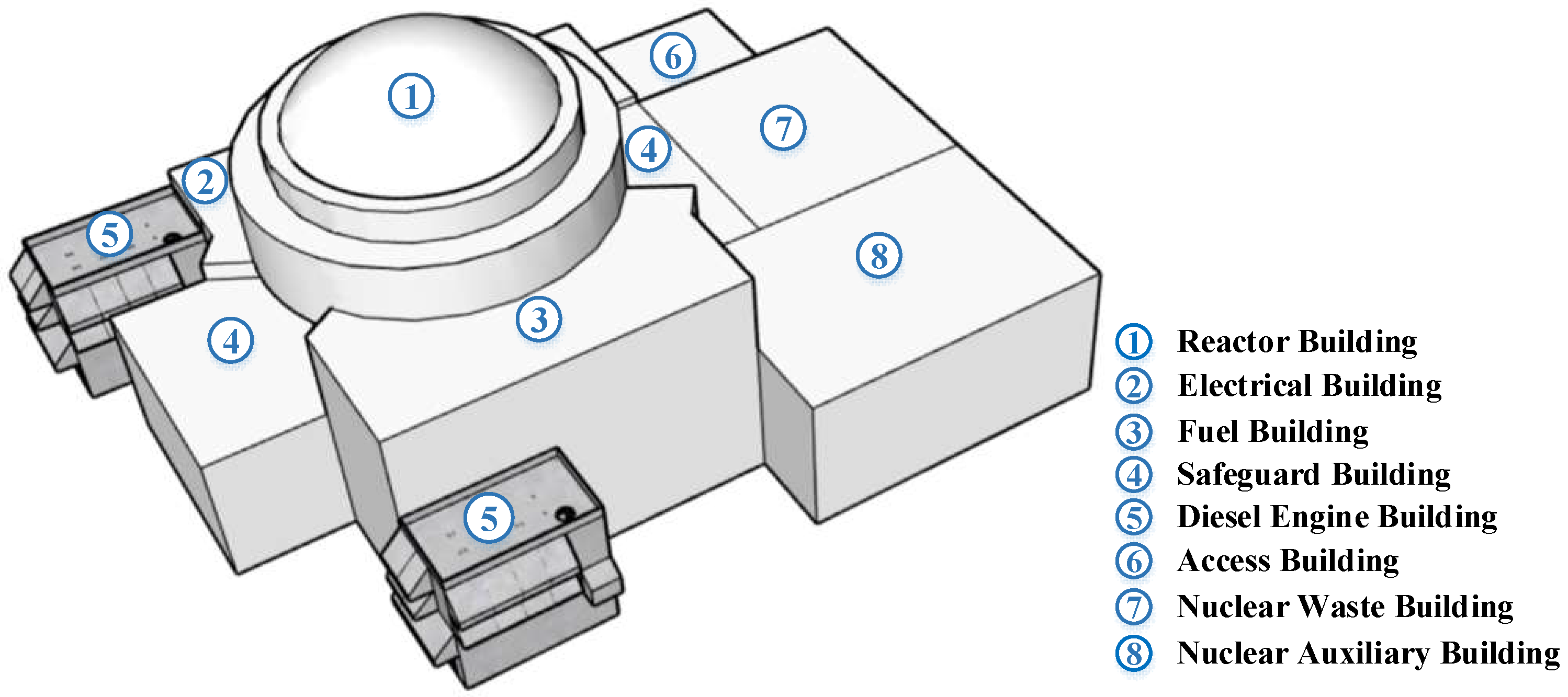
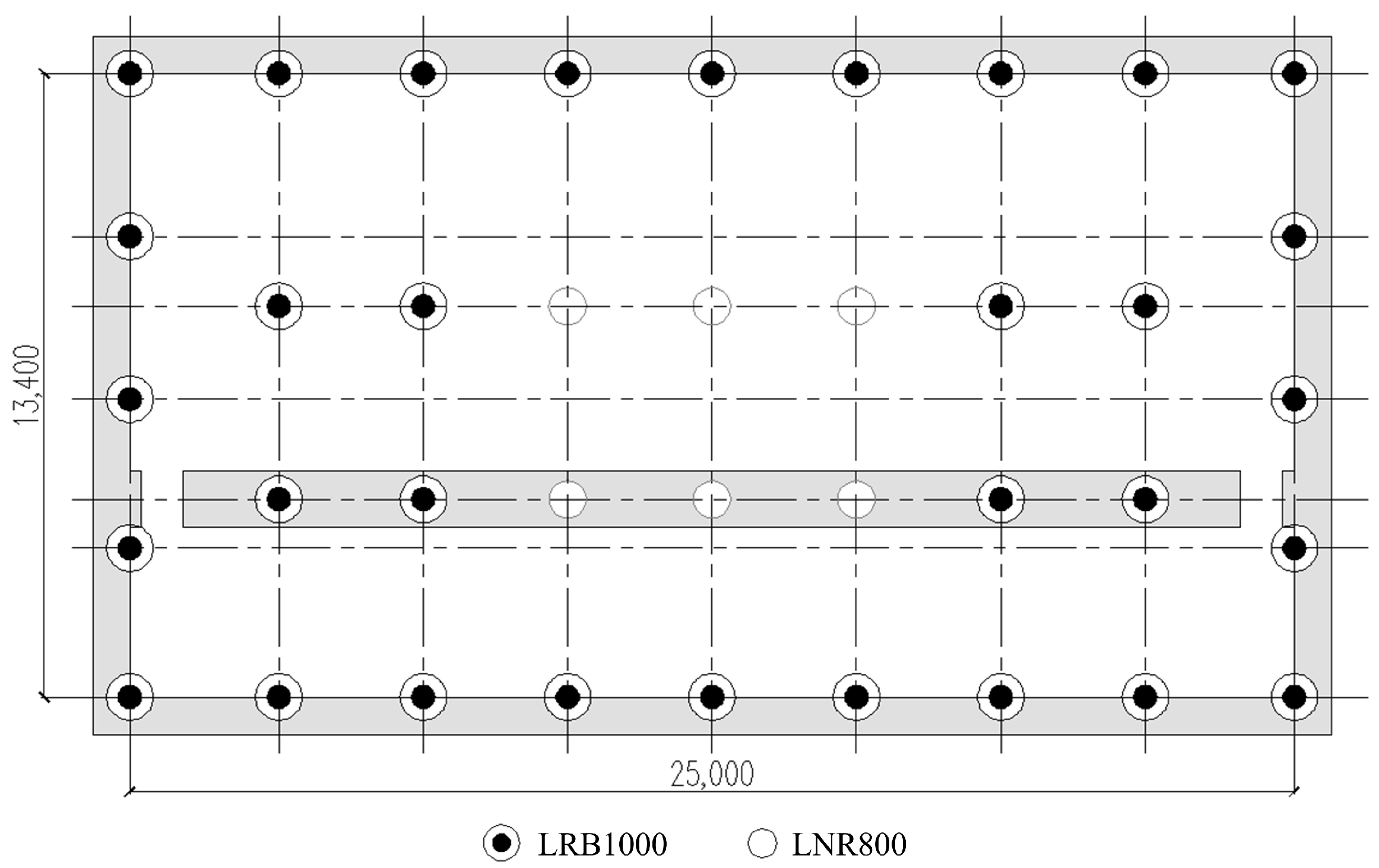
2.1. Prototype Introduction

The seismic prototype of the test structure is the diesel engine building of a nuclear power plant, which is a reinforced concrete shear wall structure and adopts raft foundation. The total weight of the structure is about 14,246 t, the plane size of the structure is 26.60 m × 15.00 m, and the overall structure is divided into two parts above ground and below, with the highest five floors above ground 24.30 m. The bottom surface elevation of the bottom plate of the underground two layers is −12.60 m, and the total height is 36.9 m. The isolation layer is added on the basis of the seismic structure. The design isolation layer is composed of 6 natural rubber bearings (LNR800) in the middle and 32 lead rubber bearings (LRB1000) in the periphery. The layout diagram of the isolation bearings is shown in Figure 2.

2.2. Model Design and Production

Due to the large plane scale and total weight of the prototype structure, and in order to reduce the test error caused by the scaling effect, it is necessary to choose the shaking table with a large table and large bearing capacity as much as possible. The main technical parameters of the shaking table are shown in

Table 1. Main technical parameters of the shaking table.

Table Size		5 m × 5 m
Vibration direction		3 directions and 6 degrees of freedom
Table weight		30 T
Maximum specimen mass		60 T
Working frequency range		0.1~50 Hz
Maximum overturning moment		1200 kN·m
Vertical performance	Displacement	±200 mm
	Speed	±1000 mm/s
	Acceleration	±1.2 g
Horizontal performance	Displacement	±400 mm
	Speed	±1200 mm/s
	Acceleration	±1.5 g

.

After considering the structural test requirements, this test selected a 5 m × 5 m shaking table and designed the experimental model at a scale of 1/8. Due to transportation restrictions, the model was disconnected from the upper and lower parts at level 7 and assembled at the test site. Due to the high reinforcement ratio of the prototype structure, the steel bars of the scaled model are still reinforced by ordinary steel bars in accordance with the principle of equivalent bending capacity, and the prototype C45 concrete is replaced by CGM high-strength, non-shrinkage grouting material with samaller particle size than the particle concrete, which is convenient for dense pouring. The elastic modulus similarity coefficient is 1/1.3. The maximum specimen mass that can be carried by the shaking table is 60 t. The experimental model is designed using an artificial mass model, and the equivalent density similarity coefficient is 1/0.505. The remaining similarity coefficients are derived using the method of dimensional analysis, and the results are shown in

Table 2. The scale factors.

Variable	Scale Factor Model/Prototype	Value	Variable	Scale Factor Model/Prototype	Value
Length	$S_l$	1/8	Frequency	$S_f={\left(S_E{S}_l{S}_m^{-1}\right)}^{0.5}$	4.984
Equivalent density	$S_{\rho }$	1/0.505	Time	$S_t=S_f^{-1}$	0.201
Modulus of elasticity	$S_E$	1/1.3	Acceleration	$S_a=S_l{S}_t^{-2}$	3.106
Stress	$S_{\sigma }=S_E$	1/1.3	Damping	$S_c=S_m{S}_t^{-1}$	0.019
Mass	$S_m=S_{\rho }{S}_l^3$	0.004	Force	$S_F=S_{\sigma }{S}_l^2$	0.012
Stiffness	$S_K=S_E{S}_l$	0.096	Moment	$S_M=S_{\sigma }{S}_l^3$	0.002

.

After the isolation layer of the test model is designed by the similarity ratio, the same number of isolation bearings are adopted and arranged in the position of the test model’s bottom plate corresponding to the isolation layer of the prototype structure. Model isolation bearings LNR140 and LRB140 correspond to prototype bearings LNR800 and LRB1000, respectively.

2.3. Connection Structure of Isolation Layer and Superstructure

In order to facilitate the installation of the isolation bearing, the isolation layer and the superstructure are connected by a number of transition plates, and connecting bars are installed between the adjacent transition plates to maintain the integrity of the isolation layer. The installation diagram of the isolation layer is shown in Figure 3a,c. From top to bottom, they are the base slab of superstructure, rubber bearings, buttresses or force sensors, base board, and shaking table. Figure 3b shows the actual installation effect of the isolation layer, and Figure 3d is the schematic diagram of the connection between the non-isolated model and the shaking table.

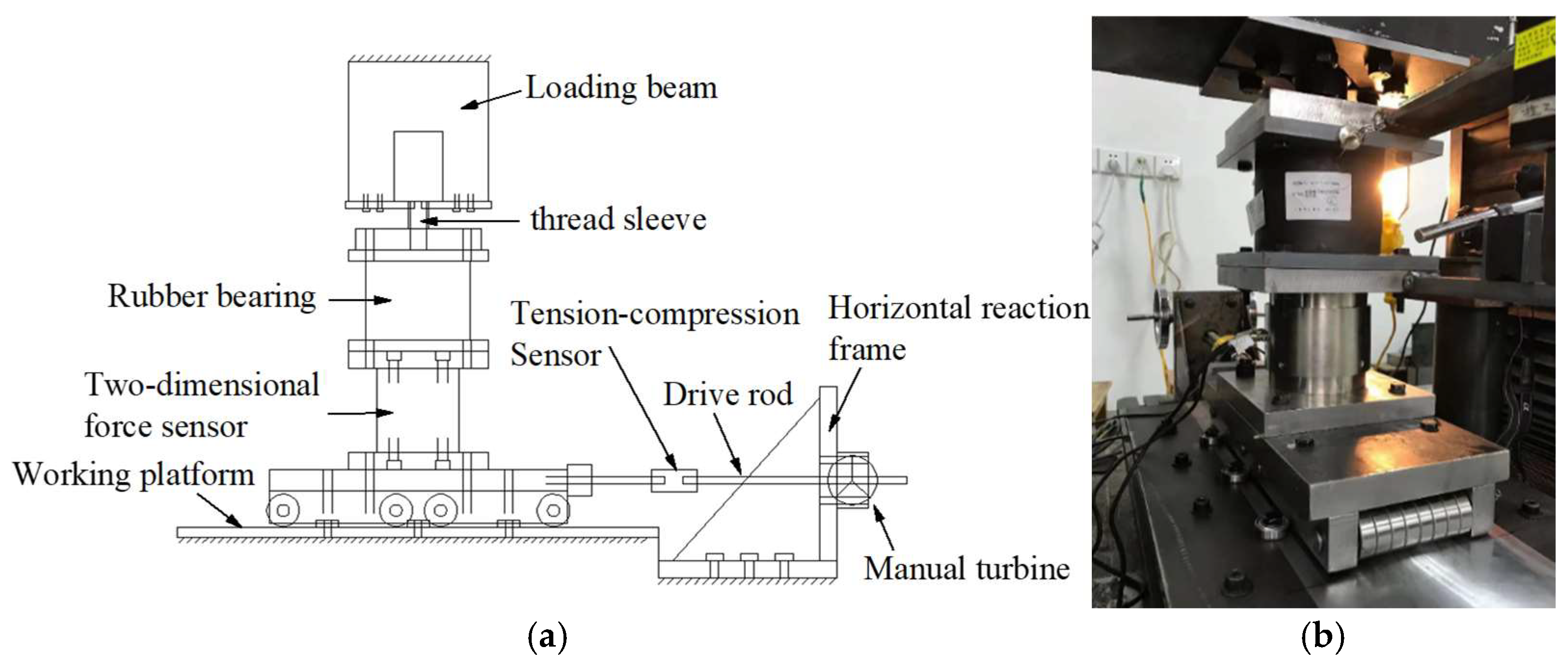
2.4. Mechanical Properties Test of Model Bearing

There are some differences between the mechanical properties of the scaled model bearing and the conventional bearing, so the compression–shear test device designed by ourselves is used to carry out the vertical compression test and compression–shear test on the same batch of isolation bearings used in the shaking table test, as shown in Figure 4. The compressive stress of the vertical compression test is 2 MPa, 4 MPa, and 6 MPa. The vertical stiffness of the LRB and LNR measured is shown in

Table 3. Vertical compressive stiffness of bearings.

Compressive Stress (MPa)	Vertical Compressive Stiffness (N/mm)
	LNR01	LNR02	Mean	LRB01	LRB02	Mean
2	131,612	145,724	138,671	181,710	133,064	157,390
4	105,531	131,250	118,393	130,933	131,522	131,233
6	108,690	126,672	117,682	144,203	137,420	140,813

.

The compression shear test was conducted on two types of bearings under static repeated loading conditions of variable pressure and variable shear angle. The horizontal stiffness of LNR specimens and the equivalent horizontal stiffness, post yield stiffness, yield force, and equivalent damping ratio of LRB specimens were tested. According to the GB/T 20688.1-2007 “Rubber bearings-Part 1: Seismic-protection isolators test methods” [32], the test was carried out under the conditions of variable pressure (1~5 MPa) and the same shear strain (100%) and then under the conditions of the same compressive stress (1 MPa) and the variable shear angle (50%, 100%, 150%, and 180%). The test results are shown in

Table 4. Compressive shear test results of rubber bearing.

Compressive Stress	Shear Strain	Horizontal Stiffness (N/mm)						Yield Strength (kN)			Equivalent Damping Ratio (%)
(MPa)	(%)	LNR01	LNR02	Mean	LRB01	LRB02	Mean	LRB01	LRB02	Mean	LRB01	LRB02	Mean
1	100	150.41	163.75	157.08	185.4	189.12	187.26	1.131	1.125	1.128	7.70	7.41	7.56
2	100	140.13	154.19	147.16	173.71	181.59	177.65	1.136	1.028	1.082	8.17	7.65	7.91
3	100	126.66	146.25	136.455	165.55	180.14	172.845	1.178	1.062	1.12	9.47	8.61	9.04
4	100	127.22	138.53	132.875	160.46	171.26	165.86	1.264	1.19	1.227	10.73	10.69	10.71
5	100	124.57	130.68	127.625	155.23	164.46	159.845	1.468	1.329	1.3985	13.61	12.81	13.21
1	50	150.41	163.75	157.08	186.09	193.13	189.61	0.695	0.707	0.701	9.07	9.14	9.11
1	100	155.92	150.41	153.165	185.4	189.12	187.26	1.131	1.125	1.128	7.70	7.41	7.56
1	150	142.24	132.71	137.475	157.43	163.06	160.245	1.164	1.16	1.162	9.35	9.45	9.40
1	180	—	130.66	130.66	143.02	154.23	148.625	1.227	1.27	1.2485	10.41	10.10	10.26

. The parameters of the model isolation bearing tested through the mechanical performance test are shown in

Table 5. Mechanical performance parameters of model isolation bearings.

Parameters	LNR140	LRB140
Compression stiffness σ = 2 Mpa (N/mm)	138,671	157,390
Horizontal stiffness γ = 100% (N/mm)	157.08	187.26 *
Yield strength (kN)	-	1.128
Equivalent damping ratio	-	7.56%

* LRB140 horizontal stiffness represents equivalent horizontal stiffness.

.

3. Shaking Table Test

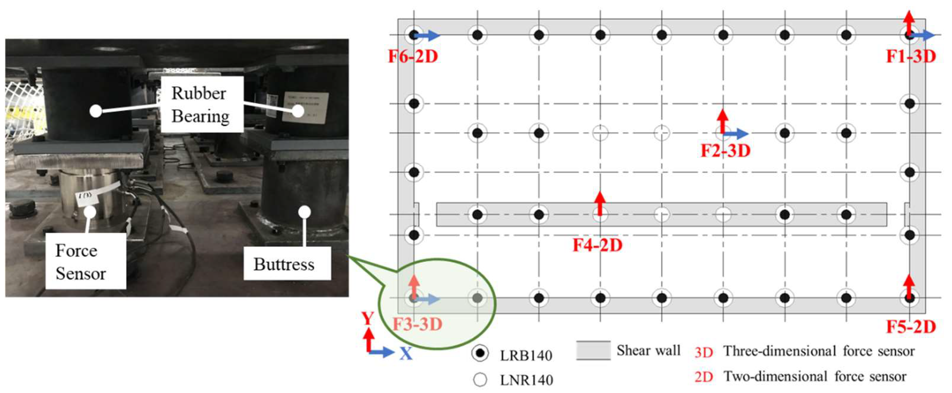
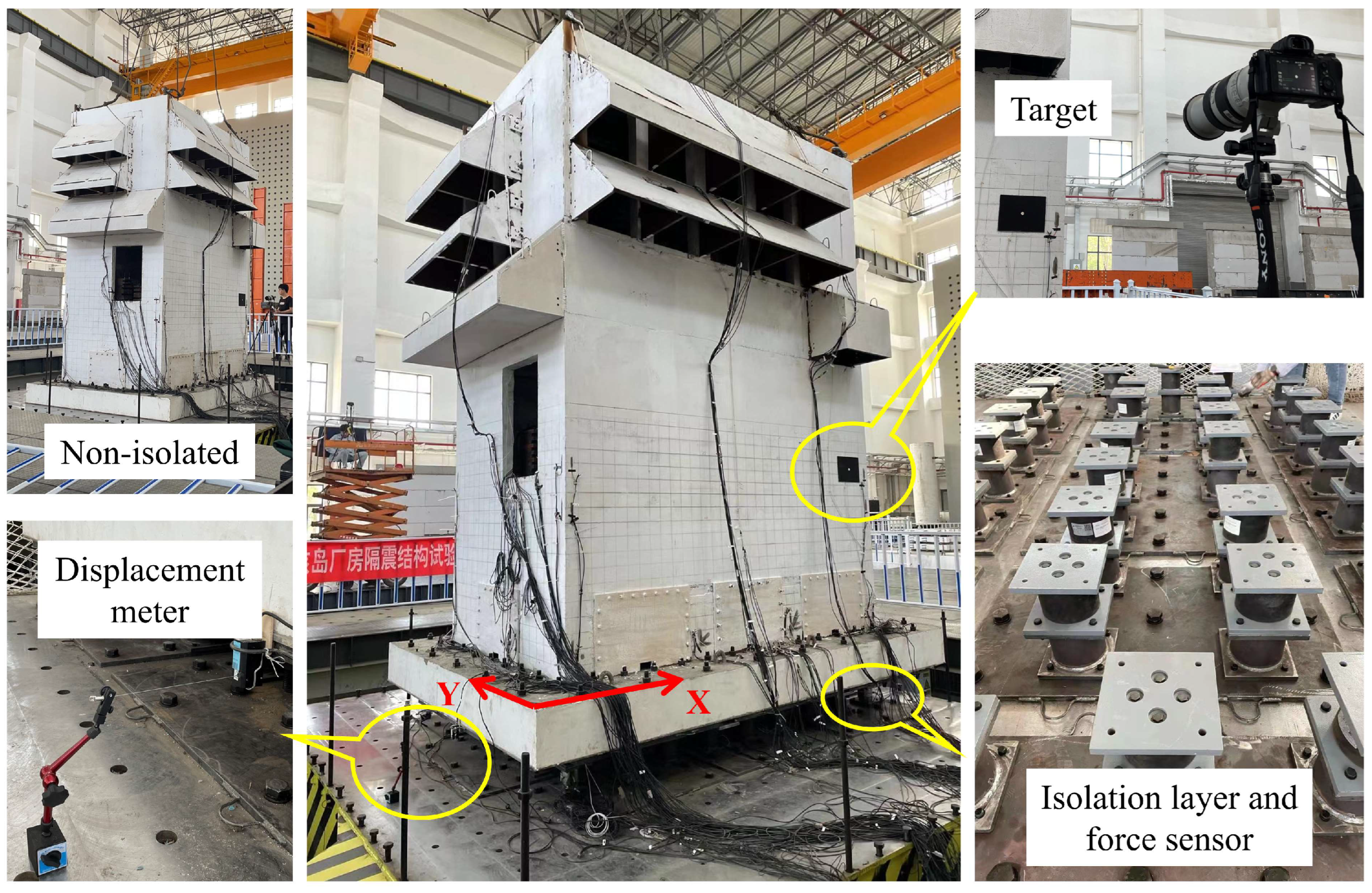
3.1. Sensor Layout and Measurement Method

The axial force and horizontal force of the isolation layer of the test model are collected by multi-dimensional force sensors, LRB at the corner points, and LRN in the middlesare respectively selected for measurement. The three-dimensional force sensor can measure the three-directional force of the bearings, and the two-dimensional force sensor can measure the axial force and a unidirectional horizontal force. The layout of the isolation bearings in the experimental model, as well as the arrangement and collection direction of the multi-dimensional force sensors, are shown in Figure 5.

The horizontal displacement of the isolation layer in two directions is measured by a cable displacement meter. Two cable displacement meters are arranged in the X and Y-directions of the upper structure bottom plate fixed to the isolation layer to measure the horizontal displacement in both directions, as shown in Figure 6.

The test model of the isolation structure removes the bottom isolation layer, and the superstructure is the seismic test structure model. Therefore, the sensor arrangement of the superstructure of the isolation test model and the seismic test structure is the same. In addition to the three-dimensional accelerometer arranged on the shaking table, the acceleration measurement is also carried out on six floors of the superstructure; each floor is arranged with seven accelerometers, and three accelerometers are located at the floor’s corner No. 7 position to measure the three directions. Another is located at the middle edge of the floor No. 6 position to measure the Z-direction acceleration, and the remaining three accelerometers are located at the middle of the floor No. 5 position to measure the three directions of acceleration. The position of the accelerometers on each floor is the same, but it is slightly changed due to the placement of the counterweight, as shown in the position of the blue square in Figure 7.

Two targets, T-X and T-Y, were set on the external wall near the No. 7 accelerometer layout point on the 4th floor of the superstructure of the test model. The target video was shot by the camera, and the time–history curve of the target position was calculated by the Photo-DSPer.m program developed by our research group using MATLAB R2018b software, so as to achieve the purpose of video monitoring of the displacement. In addition, the time–history curve will also be calibrated with the displacement of the acceleration integral of the No. 7 layout point on the 4th floor to ensure the accuracy of the displacement.

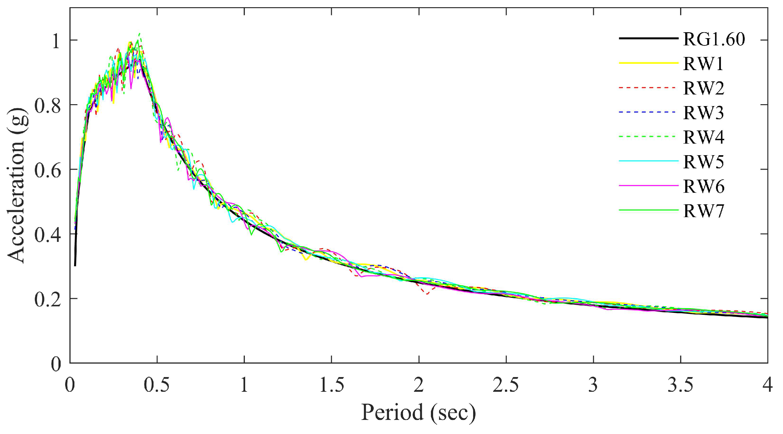
3.2. Ground Motion Selection

Seven groups of three-dimensional artificial waves (RW1~RW7) [33] were selected for the test. Each group of waves was fitted according to the RG1.60 standard spectrum [34] with a damping ratio of 5% and a PGA of 0.3 g. Different components were used in the three directions, and the peak acceleration ratio was 1:1:1. The response spectrum curve of the artificial wave is shown in Figure 8, which can be well fitted with the RG1.60 response spectrum.

3.3. Test Conditions

In order to better compare the isolation effect, the loading conditions of the non-isolation test and isolation test are set the same. In accordance with the design parameters related to the site of this research project and HAD 102/02-2019, the diesel engine building of a nuclear power plant is the seismic category I items related to nuclear safety and should be designed for seismic resistance according to the ultimate safety seismic motion (SL-2) of the site. The loading scheme of this experiment considers three seismic levels: operational safety ground motion, SL-1; ultimate safety ground motion, SL-2; and beyond design benchmark ground motion, BDBE [35]. White noise with a peak acceleration of 0.1 g in three directions is input before and after each seismic level for frequency scanning to obtain the dynamic characteristics of the model, with a total of 42 operating conditions. The peak acceleration of the prototype is 0.1 g (SL-1), 0.3 g (SL-2), and 0.5 g (BDBE), and the input peak acceleration of the test shaking table is adjusted to 0.311 g, 0.932 g, and 1.55 g, respectively.

The SL-1 level ground motion mainly studies the seismic response characteristics of isolated and non-isolated structures under different seismic waveforms, the amplification degree of bidirectional and triaxial loading to unidirectional loading, and the working effect of the hysteretic curves of LNR and LRB. Therefore, seven artificial waves were arranged for one-way input, horizontal two-way input, and three-way input along X and Y, totaling 28 working conditions.

The SL-2 level ground motion arranged seven artificial-wave, three-way seismic inputs in a total of seven working conditions, mainly to study the dynamic response of the structure, the dynamic amplification caused by the three-way loading, and assess the safety of the isolation bearing.

According to the maximum function of the shaking table, the BDBE level ground motion has arranged three working conditions of a 1.55 g horizontal-acceleration Y input, which is mainly to assess the isolation layer and the dynamic amplification of the structure. The test conditions are shown in

Table 6. Test conditions.

Seismic Level	Working Condition	Input Seismic Wave	PGA/g
			X-Direction	Y-Direction	Z-Direction
-	1	White Noise	0.1	0.1	0.1
SL-1	2~8 *	RW1~RW7 *	-	0.311	-
	9~15	RW1~RW7	0.311	-	-
	16~22	RW1~RW7	0.311	0.311	-
	23~29	RW1~RW7	0.311	0.311	0.311
-	30	White Noise	0.1	0.1	0.1
SL-2	31~37	RW1~RW7	0.932	0.932	0.932
-	38	White Noise	0.1	0.1	0.1
BDBE	39~41	RW1\RW5\RW7	-	1.55	-
-	42	White Noise	0.1	0.1	0.1

* The abbreviated working condition numbers correspond to artificial waves 1 to 7 in order. For example, in the SL-1 level ground motion, working condition 2 corresponds to artificial wave RW1, working condition 3 corresponds to artificial wave RW2, etc. The other seismic levels are expressed in the same way.

.

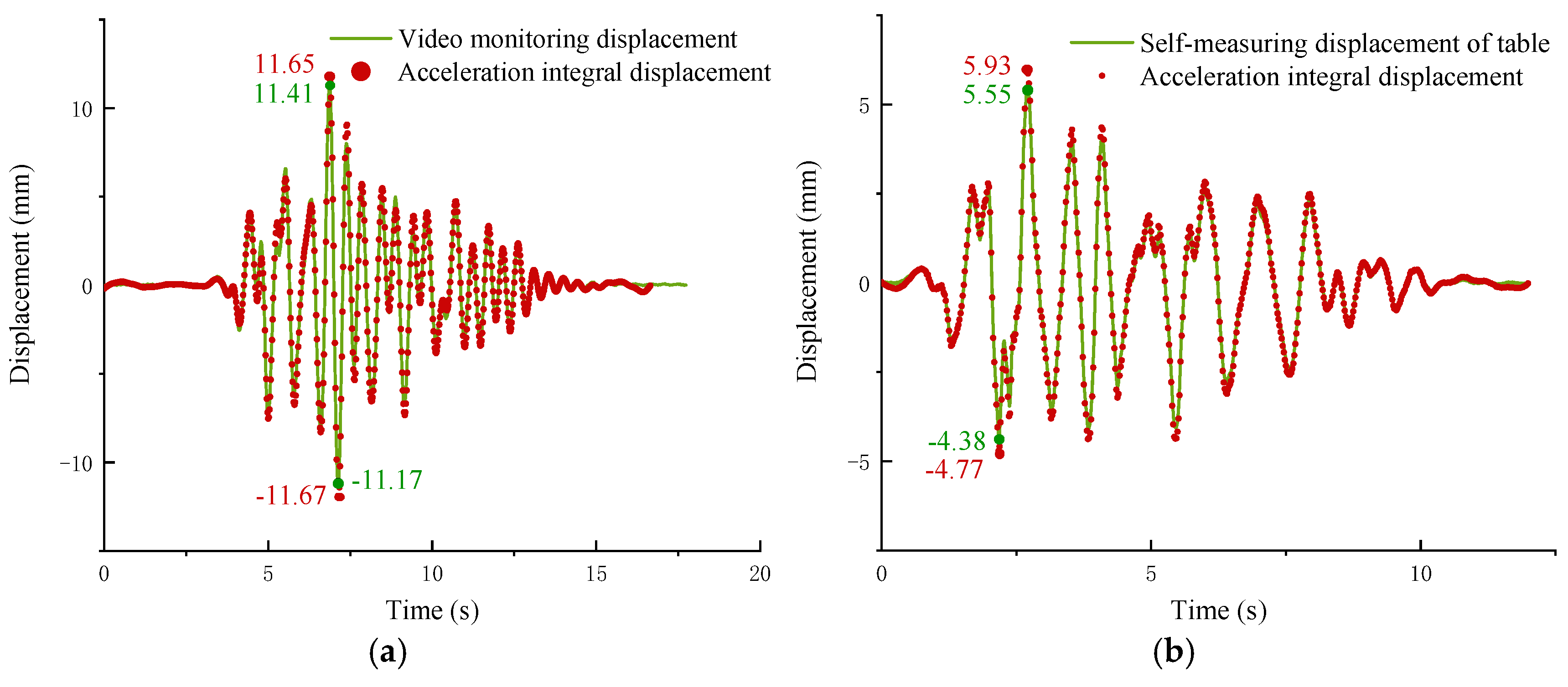
3.4. Data Processing and Calibration

Considering the height of the test model and the convenience of the installation method of the measuring instrument, the displacement result of the corresponding position is usually obtained by integrating the acceleration. In order to avoid the high frequency noise in the acceleration data affecting the accuracy of the displacement and other results, the acceleration should be filtered according to the actual performance of the shaking table. In order to determine the appropriate filtering range, working condition 3 was selected. The integrated displacement of the floor accelerometer signal was compared with the video monitoring displacement, and the integrated displacement of the shaking table accelerometer signal was compared with the self-measured displacement of the table. The calibration structure is shown in Figure 9. Finally, the filtering range suitable for this experiment was selected as 0.5–50 Hz.

4. Test Results

4.1. Model Dynamic Characteristic Analysis

Before inputting seismic motion, a 0.1 g white noise sweep was used to obtain the dynamic characteristics of the experimental model through transmission analysis, as shown in

Table 7. Dynamic characteristics of the model structure.

Test Model	First Order Frequency Y-Direction	Second Order Frequency X-Direction	Third Order Frequency Twist	Fourth Order Frequency Y-Direction
Isolation model	2.30 Hz	2.33 Hz	2.42 Hz	12 Hz
Non-isolated model	27 Hz	32 Hz	45 Hz	50 Hz

. The first mode of the model is Y-translational, the second mode is X-translational, and the third mode is torsional.

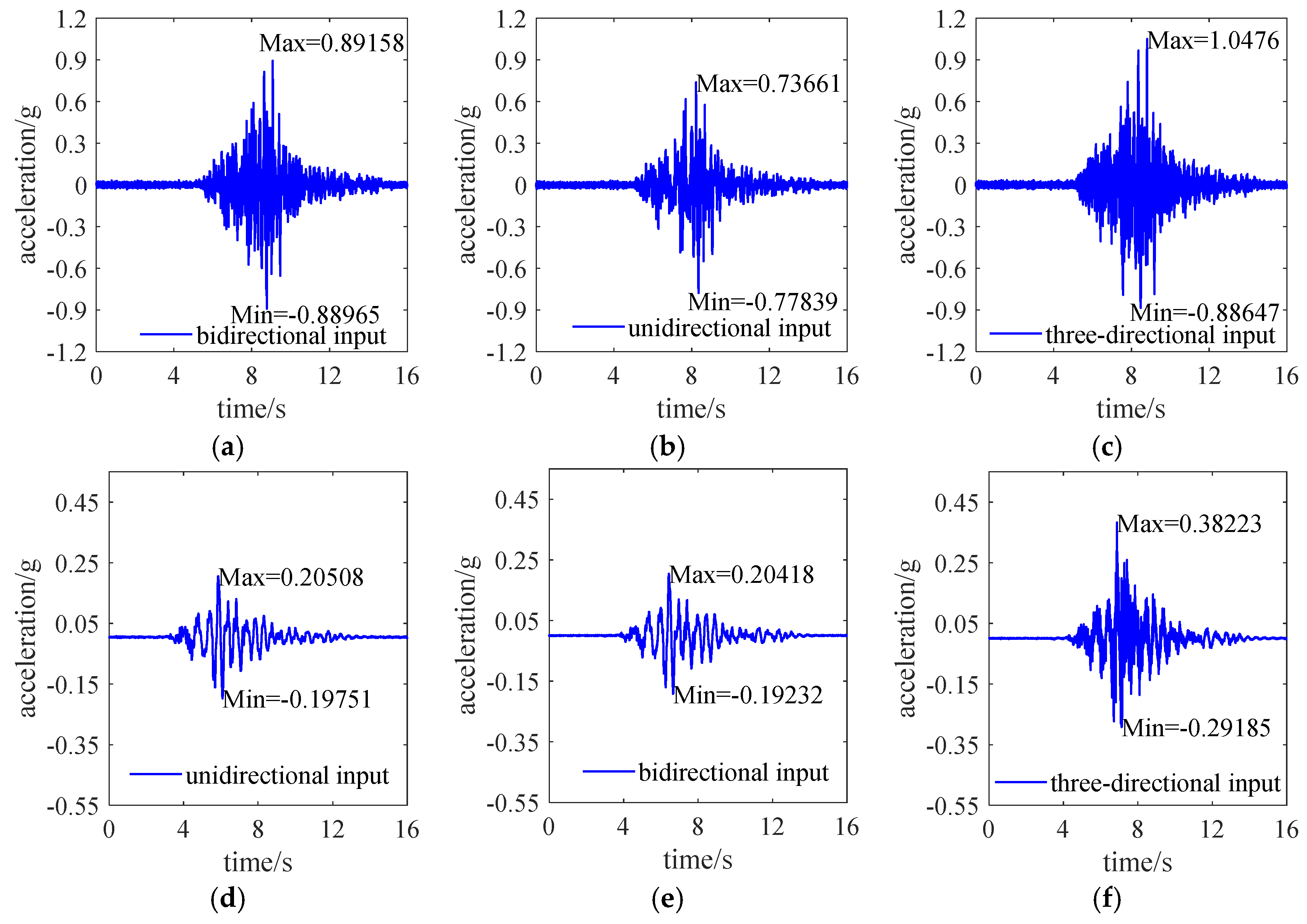
4.2. Acceleration Response

In order to explore the overall effect of seismic isolation of the test model, the acceleration peak value collected from the No. 5 acceleration measurement point in the middle of each floor of the test model are taken to obtain the acceleration envelope curve under each working condition, as shown in Figure 10. The working conditions were divided into six groups according to different ground motion levels and input directions. Each group contained seven groups of artificial waves except that the BDBE level ground motion only contained RW1, RW5, and RW7. The envelope diagrams of both isolated and non-isolated models include acceleration on the 0th floor (shaking table top), 1st floor (model base), 2nd floor, 4th floor, 6th floor, 7th floor, and 9th floor. The isolation model includes an isolation layer, so the height of the first floor is higher than that of the non-isolated model.

As shown in the figure, the acceleration in the X and Y-directions of the non-isolated model shows a significant increasing trend with the increase in floor height, demonstrating the characteristic of dynamic amplification of non-isolated structures, and the increase in earthquake level makes this trend greater. The acceleration envelope diagram of the isolation model shows that the acceleration envelope below an elevation of 3 m (6 floors) is relatively evenly distributed along the height, reflecting the characteristics of the isolated rigid structure. But there is an increase in the acceleration envelope at an elevation of 3–3.5 m. After observation and analysis, it is believed that this area is located in the assembly layer, and there are some shrinkage cracks on the surface of the post-poured concrete and changes in the connection stiffness. The protruding window on the upper wall also causes an increase in the moving mass and moment of inertia, resulting in a change in the regularity of the dynamic response of this layer. The reason why this phenomenon did not occur in non-isolated structures is that, in order to ensure the consistency of the total mass of the two models, after removing the isolation layer of the isolated model, weights were added, and some weights were placed on the top of the structure.

To investigate the seismic response of isolated and non-isolated structures under unidirectional horizontal, bidirectional horizontal, and tri-directional seismic inputs, the same artificial wave RW5 was selected under SL-1 level ground motion. The acceleration time history in the Y-direction of the 9th floor of the structure under different working conditions was analyzed. Figure 11 shows the processed acceleration time–history curves. It can be observed that the peak acceleration of the non-isolated model under bidirectional horizontal seismic input is approximately 15% larger than that under unidirectional horizontal seismic input, and the peak acceleration under tri-directional seismic input is about 21% larger than that under bidirectional horizontal seismic input, indicating a significant amplification of peak acceleration in the non-isolated model under multi-directional seismic inputs. For the isolated model, the peak acceleration under bidirectional horizontal seismic input is essentially the same as that under unidirectional horizontal seismic input, but the tri-directional seismic input has a greater impact on the peak acceleration of the isolated structure, increasing it by 0.18 g compared to the bidirectional horizontal seismic input. Under the same conditions, the ratio of the peak acceleration of the isolated model to that of the non-isolated model at the same location is defined as the isolation rate. In Figure 11, the isolation rate under the unidirectional horizontal seismic input for condition 6 is about 26%; for condition 20 under the bidirectional horizontal seismic input, it is about 23%, and for condition 27 under the tri-directional seismic input, it is about 36%.

The isolation rates for the peak accelerations at the top of the structure under other conditions are listed in

Table 8. Isolation rate of the top layer of the test model.

Seismic Level	Ground Motion Input	Direction	RW1	RW2	RW3	RW4	RW5	RW6	RW7	Mean Value
SL-1	Unidirectional	X	0.25	0.20	0.21	0.25	0.21	0.23	0.23	0.22
		Y	0.29	0.21	0.31	0.30	0.26	0.26	0.25	0.27
	Bidirectional	X	0.25	0.22	0.22	0.22	0.20	0.23	0.25	0.23
		Y	0.26	0.19	0.25	0.28	0.23	0.24	0.23	0.24
	Three- dimensional	X	0.57	0.37	0.46	0.33	0.42	0.50	0.52	0.45
		Y	0.59	0.37	0.69	0.34	0.37	0.41	0.59	0.48
		Z	1.55	1.54	1.51	1.36	1.41	1.67	1.69	1.53
SL-2	Three- dimensional	X	0.29	-	0.41	0.33	0.29	-	0.38	0.34
		Y	0.43	0.29	0.41	0.31	0.30	0.34	0.32	0.35
		Z	0.98	1.27	1.54	1.52	0.86	1.09	1.22	1.21
BDBE	Unidirectional	Y	0.24	-	-	-	0.18	-	0.21	0.21

. Under SL-1 level ground motion, the average isolation rate for unidirectional and bidirectional horizontal seismic inputs is about 23.5%, while, under tri-directional seismic input, the average horizontal isolation rate is 46.5%, and the vertical isolation rate is 153.4%, indicating good horizontal isolation effectiveness of the isolated structure, with better isolation effectiveness in the X-direction than in the Y-direction, and an amplification phenomenon in vertical acceleration compared to the non-isolated structure. The average horizontal isolation rate under SL-2 level ground motion is about 35%, which is 11.5% lower than that under SL-1 level ground motion’s tri-directional input conditions, and the average vertical isolation rate is 32% lower than that under SL-1 level ground motion’s tri-directional input conditions. However, the average isolation rate for unidirectional horizontal input under BDBE level ground motion remains at 21%, which is essentially the same as that under SL-1 level ground motion’s unidirectional input conditions, demonstrating that the isolation layer still provides good isolation effectiveness under high seismic levels.

The Y-direction acceleration response spectra for each floor under tri-directional input conditions 29 and 37 of artificial wave RW7 for SL-1 and SL-2 level ground motions are shown in Figure 12. The floor response spectra of the isolated structure are similar across all floors, and the response spectra increase with height. The peak frequencies of the response spectra for the isolated structure are consistent, and the peak values of the response spectra are significantly reduced compared to those of the non-isolated structure. For example, under SL-1 level ground motion, the Y-direction peak of the 9th floor occurs near 1.8 Hz, with a response spectrum peak of 0.86 g. Under the same condition, the peak frequency for the Y direction of the 9th floor in the non-isolated structure is 11.84 Hz, with a corresponding response spectrum value of 2.30 g. Under SL-2 level ground motion, the Y-direction response spectrum peak frequency for the 9th floor of the isolated structure is 1.56 Hz, with a response spectrum peak of 1.81 g. Under the same condition, the peak frequency for the Y-direction of the 9th floor in the non-isolated structure is 50.88 Hz, with a corresponding response spectrum value of 8.22 g. For frequencies below 3 Hz, the Y-direction floor response spectra of the isolated structure are higher than those of the shaking table surface. However, for frequencies above 3 Hz, the floor response spectra values are lower than those of the shaking table surface, demonstrating excellent isolation effectiveness.

Figure 13 compares the X-direction acceleration response spectra of the same floor for the isolated and non-isolated models. Under SL-1 level ground motion, the X-direction floor response spectra of the isolated structure are higher than those of the non-isolated structure for frequencies below 2.66 Hz. Beyond this frequency range, the floor response spectra values of the isolated structure are lower than those of the non-isolated structure. The comparison of response spectra for the two models under SL-2 level ground motion exhibits the same characteristics, but the frequency at which the response spectra of the isolated model begin to fall below those of the non-isolated model is lower, at 1.93 Hz. Based on the frequency similarity ratio of 4.984 for this experiment, it is known that for the prototype structure, frequencies exceeding 0.53 Hz under SL-1 level ground motion and 0.39 Hz under SL-2 level ground motion result in significantly reduced acceleration response spectra for the isolated model compared to the non-isolated model, indicating good isolation effectiveness. The predominant frequency range for the response spectra of the 2nd and 6th floors of the isolated model under both seismic levels is 1.61–1.87 Hz, which is close to the natural frequency of the isolated model at 2.30 Hz, corresponding to a frequency range of 0.32–0.38 Hz for the prototype structure. The 9th floor exhibits greater seismic response, with a predominant frequency range for the isolated response spectra of 25.89–26.83 Hz, corresponding to a frequency range of 5.19–5.40 Hz for the prototype structure. All floors effectively avoid the main operating frequency range of the equipment, which is 10–20 Hz [22].

Under the SL-1 level ground motion, the peak response spectra of the non-isolated model on the 2nd, 6th, and 9th floors are 1.38 times, 1.56 times, and 2.56 times those of the isolated model on the same floors, respectively. Under the SL-2 level ground motion, the peak response spectra of the non-isolated model on the 2nd, 6th, and 9th floors are 2.50 times, 2.39 times, and 3.39 times those of the isolated model on the same floors, respectively. Therefore, under the same conditions, the higher the floor, the greater the reduction in the response spectra of the non-isolated model, and the better the isolation effectiveness. For the isolated model, under higher seismic levels, the proportion of the peak response spectra on the same floor compared to the non-isolated model is even smaller, indicating that the isolation system continues to provide excellent isolation performance.

The vertical floor acceleration response spectra for both the isolated and non-isolated models are shown in Figure 14. Under SL-1 and SL-2 level ground motions, the predominant frequencies of the acceleration response spectra for the two models do not vary significantly. For the isolated model, the predominant frequency range across all floors is 21.99–24.99 Hz, which is close to the vertical frequency of the isolated model at 30.5 Hz, corresponding to a prototype frequency range of 4.41–5.01 Hz. For the non-isolated model, the predominant frequency range across all floors is 50.88–52.73 Hz, with a vertical frequency of 82.50 Hz. The isolated model reduces the predominant frequency of the vertical acceleration response spectra compared to the non-isolated model. However, due to the relatively high vertical stiffness of the isolation layer, the floor’s predominant frequencies are close to the vertical frequency of the isolated model. As a result, the acceleration response spectra increase with floor height, making the structure more susceptible to vertical resonance. Therefore, the isolation system does not provide effective vertical vibration reduction.

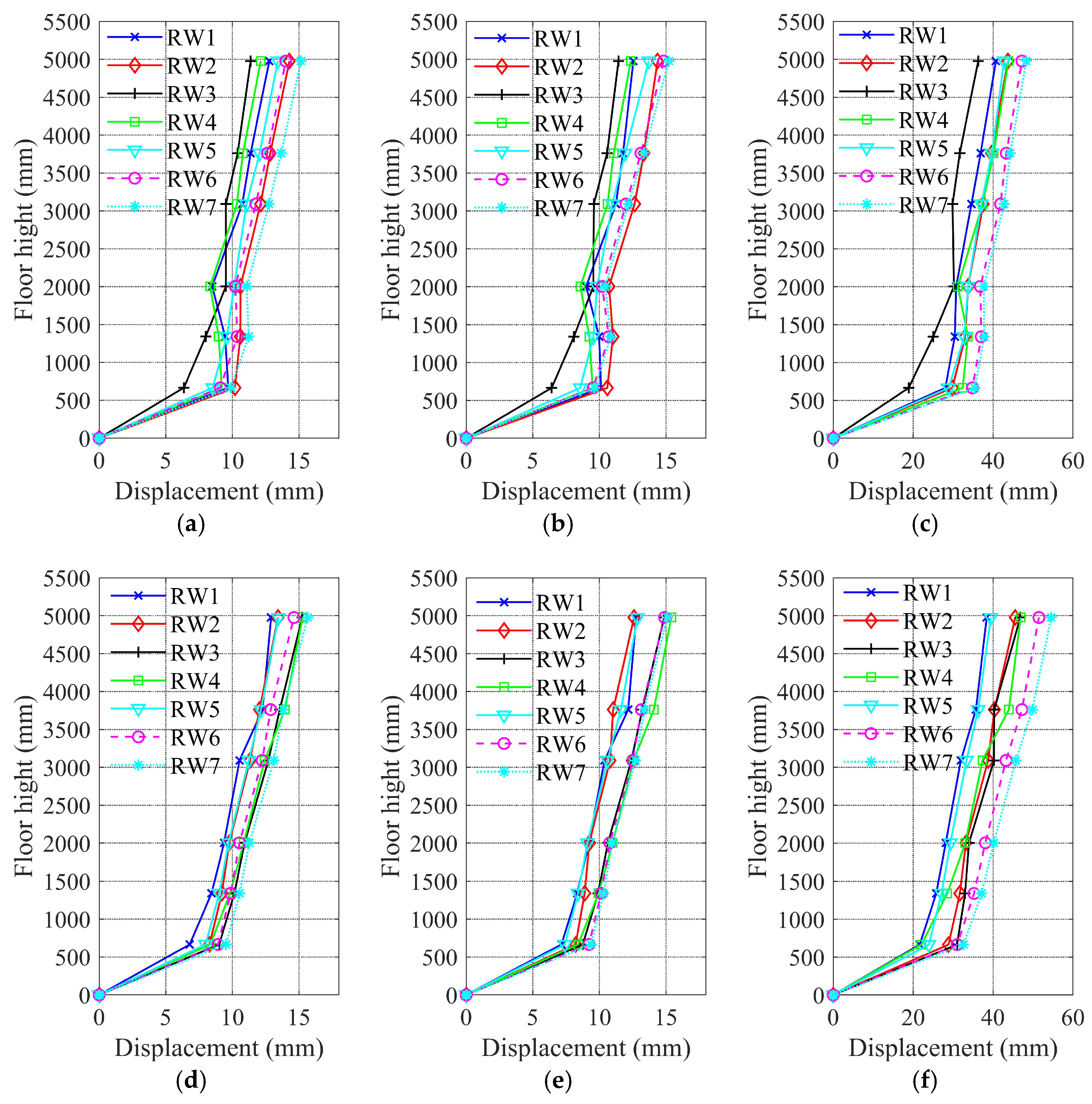
4.3. Displacement Response

Figure 15 shows the horizontal displacement time–history curves of each floor relative to the shaking table surface for the isolated model under tri-directional input of artificial wave RW1 at SL-1 level ground motion. This means that the displacement of each floor includes the displacement of the isolation layer. It can be observed that the horizontal displacement of the isolation layer (i.e., the 1st floor in the figure) is in phase with the displacements of the other floors, indicating that the displacement vibration is primarily controlled by the fundamental mode shape in that direction.

The peak displacements of each floor of the isolated structural model relative to the shaking table surface under seven sets of artificial wave conditions at different seismic levels are shown in Figure 16. The height of the 1st floor is 666 mm, which includes the isolation layer and the height of the fixed base plate. Therefore, the displacement of the 1st floor represents the displacement of the isolation layer. Under bidirectional input of SL-1 level ground motion, the average peak displacement of the isolation layer in the X-direction is 8.99 mm, and in the Y-direction, it is 8.41 mm. Under tri-directional input of SL-1 level ground motion, the average peak displacement of the isolation layer in the X-direction is 9.20 mm, and the average peak displacement in the Y-direction across the seven artificial waves is 8.36 mm. It can be seen that under SL-1 level ground motion, the impact of bidirectional and tri-directional inputs on the peak horizontal displacement of the structure is similar, with a shear strain of up to 21.9% in the bearings. Under tri-directional input of SL-2 level ground motion, the average peak displacement of the isolation layer in the X-direction is 29.76 mm, and in the Y-direction, it is 27.29 mm, with a shear strain of up to 70.9% in the bearings. Under BDBE level ground motion, the average peak displacement of the isolation layer in the Y-direction is 46.74 mm, with a shear strain of up to 111.3% in the bearings. The maximum displacement of the isolation layer at different seismic levels, when scaled to the prototype using the similarity ratio, is 373.92 mm, which meets the target of being less than the 400 mm collision avoidance gap.

The horizontal deformation of the isolated model is primarily concentrated in the isolation layer. Under tri-directional input of SL-1 level ground motion, the maximum story drift ratio of the superstructure is 1/301. Under tri-directional input of SL-2 level ground motion, the maximum story drift ratio is 1/91. Under unidirectional input of BDBE level ground motion, the maximum story drift ratio is 1/81. Compared to the maximum horizontal displacement of the isolation layer, the superstructure behaves almost like a rigid body, with the isolation layer playing a major role in absorbing seismic energy. However, the peak horizontal displacements of each floor increase progressively with height, indicating a certain degree of overturning effect in the superstructure.

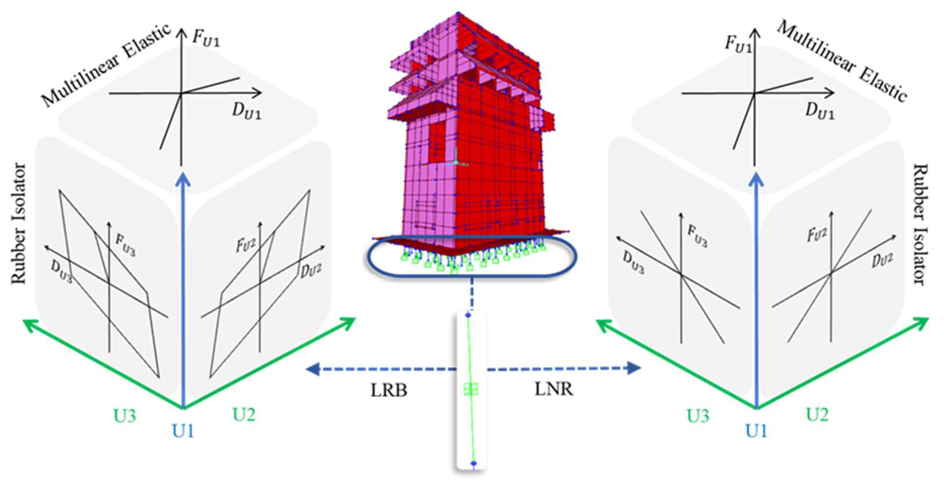
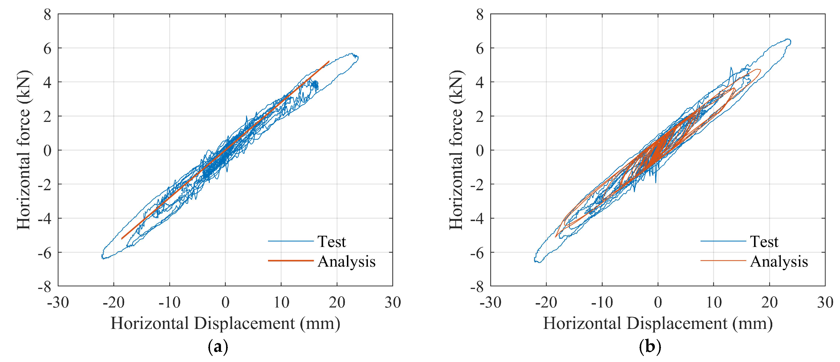
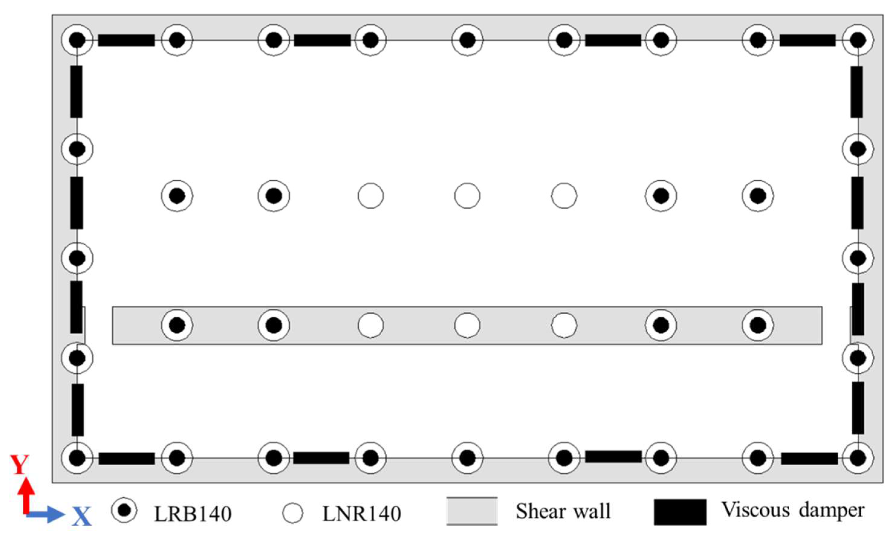
5. Finite Element Numerical Simulation

In order to compare with the data obtained from the seismic isolation model test, a finite element model consistent with the conditions of the shaking table test model was established using SAP2000 for nonlinear time–history analysis. The parameters of the structural calculation model, especially the technical parameters of the isolation bearings, were identified to ensure the accuracy of the model calculation results. The SAP2000 finite element model used shell elements and beam elements to establish the main structure model, as shown in Figure 17. The horizontal behavior of the isolation bearings was simulated using the Rubber Isolator element, while the vertical behavior was simulated using the Multilinear Elastic element. Considering the difference in stiffness of the actual isolation bearings under tension and compression, the tensile stiffness of the bearings in the finite element model was set to 1/10 of the compressive stiffness.

The finite element model conducted a nonlinear time–history analysis for the 31 working conditions under the tri-directional input of the artificial seismic wave RW1 corresponding to the SL-2 level ground motion. The actual measured shaking table acceleration was selected as the input ground motion. The modal results of the seismic isolation structure test model and the finite element model are presented in

Table 9. Modal comparison between shaking table test model and finite element model.

Mode	Test Result		Finite Element Model of Test Structure		Error
	Frequency (Hz)	Direction	Frequency (Hz)	Direction
1	2.30	Y	2.32	Y	0.8%
2	2.33	X	2.34	X	0.4%
3	2.42	Twist	2.39	Twist	−1.3%
4	12.00	Y	16.7	Y	28.1%
5	26.00	X	25.68	X	−1.3%
6	30.50	Z	44.29	Z	31.1%

. For the seismic isolation structure, the first three vibration modes play a dominant role. The first two translational periods of the finite element model and the experimental results show good agreement, and the period distribution pattern of the experimental results is consistent with that of the finite element simulation. This indicates that the finite element model of the test is reasonably constructed.

Figure 18 presents a comparison of the hysteretic curves between the finite element model and the experimental model for the LNR bearing labeled F2-3D and the LRB bearing labeled F6-2D. In the finite element simulation, the LNR bearing employs linear elements to simulate its horizontal mechanical behavior, which fails to account for the energy dissipation effects resulting from the friction and interlocking between the steel plates and rubber layers. Consequently, there are certain discrepancies between the finite element and experimental hysteretic curves for the LNR bearing. According to the hysteresis curve, the average horizontal stiffness of LNR was calculated to be 276.41 N/mm, with a standard deviation of 31.24 N/mm. On the other hand, the LRB bearing is assigned nonlinear mechanical properties through the elements, resulting in a more robust finite element hysteretic curve that exhibits a significantly more realistic response. The average post yield stiffness of LRB is 254.12 N/mm, with a standard deviation of 12.41 N/mm.

Figure 19 compares the acceleration time–history curves of the experimental and finite element models. The acceleration at the 1st floor represents the acceleration above the isolation layer, while the acceleration at the 9th floor represents the acceleration at the top of the model. Figure 19a,b show the comparison of the horizontal, X-direction acceleration at the isolation layer and the top floor, respectively. It can be observed that the waveforms and overall trends of the time–history curves from both models exhibit good agreement, with similar peak values. Figure 19c,d present the comparison of the vertical acceleration at the isolation layer and the top floor, respectively. The best fit is observed at the 1st floor, while the peak value of the finite element model at the 9th floor is larger than that of the experimental model. This discrepancy is primarily due to the fact that the vertical Multilinear Elastic element used for the bearings is a linear unit, which fails to simulate the vertical damping of the bearings.

The comparison of displacement time–history curves between the finite element model and the experimental model is illustrated in Figure 20. Horizontally, the absolute displacement peak obtained from finite element analysis for the first story was found to be 95.82% of the experimental peak value, while the peak ratio for the ninth story was observed to be 90.67%. The test results and the finite element simulation results exhibit good consistency in terms of absolute displacement waveforms and peak values during the initial and final stages of the test. However, discrepancies are observed at approximately 4 s, which can be attributed to the occurrence of peak ground motion acceleration at this moment. During the period of maximum acceleration, the metal counterweight in the test model is most susceptible to collisions, resulting in instantaneous acceleration spikes. These spikes may either amplify or attenuate the floor acceleration. However, the metal counterweight block was not modeled as a discrete entity in the finite element model, the collision phenomenon was not considered, and the displacement was obtained by integrating the acceleration. Therefore, the displacement time–history curve differed at around 4 s. Vertically, the absolute displacement peak value of the first layer test result is 95.32% of the finite element peak value, and the peak ratio of the 9th layer is 94.17%. The displacement time–history curves of both models aligned well in waveform and peak values due to the consideration of differing tension–compression stiffness in the bearings.

6. Deficiencies of Base Isolation and Suggestions for Improvement

Figure 21 shows the acceleration time–history curves of floors 1, 4, 7, and 9 under the tri-directional seismic input for working condition 31 of the isolation test. It can be observed that, as the floor height increases, the peak acceleration first decreases and then increases, indicating the presence of an overturning effect in the superstructure. The primary reason for this is that the horizontal displacement of the isolation layer leads to significant tensile displacement in the bearings, causing the superstructure to exert a substantial overturning moment on the foundation. When the isolation model is subjected to strong seismic actions, the isolation bearings are prone to tension, and the tensile stiffness of the bearings is much lower than the compressive stiffness, making the overturning effect more pronounced.

To mitigate the overturning effect in the seismic isolation structure, a viscous damper-hybrid isolation system is proposed. In this system, 16 horizontal viscous dampers are added to the isolation layer of the test model to control and reduce the overturning effect. The damping coefficient of the viscous dampers is 19 kN∙s/m, with damping exponents of 0.25, 0.4, 0.5, and 1. The arrangement of the viscous dampers is illustrated in Figure 22.

Four hybrid isolation models and the original isolation model were used to calculate the response under the tri-directional input of the RW1 wave at the BDBE level ground motion. The calculated maximum tensile stresses in the bearings and the maximum base shear forces are presented in

Table 10. Comparison between tensile stress of isolation bearing and extreme value of base shear.

Scheme	Damping Index	Maximum Tensile Stress (Mpa)	Maximum X-Direction Base Shear (kN)
1	Undamped	1.58	365.86
2	α = 0.25	1.32	312.41
3	α = 0.4	1.04	270.88
4	α = 0.5	0.89	255.19
5	α = 1	0.90	242.48

. Models of Schemes 4 and 5 exhibited the smallest tensile stresses in the bearings and the smallest base shear forces in the X-direction, with a tensile stress of 0.90 MPa, meeting the design target of keeping the tensile stress in the isolation bearings below 1 MPa under the BDBE level ground motion. The base shear force of Scheme 5 was reduced by 33.72% compared to Scheme 1.

The acceleration amplification factor diagrams for the models are shown in Figure 23. For Scheme 1, the peak floor accelerations initially decreased and then increased with floor height, indicating an overturning effect. This phenomenon was somewhat mitigated in Schemes 2 and 3, but a slight overturning effect still persisted. In Schemes 4 and 5, the peak floor accelerations increased with floor height, demonstrating an improvement in the overturning effect. Therefore, it is recommended to use viscous dampers with a damping coefficient of 19 kN∙s/m and damping exponents of 0.5 or 1.

The structural anti-overturning moment ratio, denoted as $\beta$, is defined as the ratio of the anti-overturning moment to the overturning moment. It serves as a safety reserve coefficient to verify the structure’s resistance to overturning under rare earthquake conditions. According to section 4.3.7 of the CECS126-2001 “Technical specification for seismic-isolation with laminated rubber bearing isolators” [36], the overturning moment should be calculated based on the rare earthquake action, and the anti-overturning moment should be calculated based on the representative value of the gravity load of the superstructure during the overall anti-overturning verification of the structure. The anti-overturning safety factor $\beta$ should be greater than 1.2. The formula for calculating the anti-overturning moment ratio is given by the following:

$$\beta ={\displaystyle \frac{M_R}{M_0}}$$

(1)

where $M_R$ is the anti-overturning moment and $M_0$ is the overturning moment.

The overturning moment $M_0$ formed by horizontal earthquake action in the isolation layer can be expressed by the following formula:

$$M_0=m_b\left({\ddot{x}}_b+{\ddot{x}}_g\right)h_0+{\displaystyle \sum }_{i=1}^n{m}_i\left({\ddot{x}}_i+{\ddot{x}}_g\right)h_i$$

(2)

where $m_b$ and $m_i$ are the masses of the isolation layer and the $i$-th floor, respectively; ${\ddot{x}}_b$ and ${\ddot{x}}_i$ are the relative horizontal accelerations of the isolation layer and the $i$-th floor, respectively; $h_0$ and $h_i$ represent the distances from the isolation layer and the $i$-th floor to the top surface of the foundation, respectively; and ${\ddot{x}}_g$ is the horizontal acceleration of ground motion.

The anti-overturning moment $M_R$ of the base isolation structure can be expressed by the following formula:

$$M_R=G_b\left(r_b+△x_b\right)+{\displaystyle \sum }_{i=1}^n{G}_i\left(r_i-△x_i\right)$$

(3)

where $G_b$ and $G_i$ represent the representative values of the permanent loads for the isolation layer and the superstructure at each floor, respectively, $r_b$ and $r_i$ denote the distances from the centroid of the isolation layer and the superstructure at each floor to the axis of the outermost isolation bearing, respectively, and $△x_b$ and $△x_i$ represent the horizontal offset of the center of gravity of the isolation layer and the $i$-th floor relative to the centroid at the base of the isolation layer, respectively, as determined in the dynamic analysis.

Using the five isolation schemes as computational models, the anti-overturning moment ratios under seismic excitation were calculated to evaluate the anti-overturning capabilities of each scheme. The calculation results are presented in

Table 11. Anti-overturning moment ratio of isolation structures with different damping coefficients.

Isolation Scheme	Damping Coefficient	β
1	Undamped	1.159
2	0.25	1.986
3	0.4	2.344
4	0.5	2.511
5	1	2.544

.

By calculating the anti-overturning moment ratios for the five schemes, it can be observed that Scheme 1 (without dampers) has an anti-overturning moment ratio of 1.159, which is slightly below the required threshold of 1.2. This confirms that Scheme 1 indeed has an overturning issue. In contrast, the other schemes incorporating dampers exhibit anti-overturning moment ratios greater than 1.2. Furthermore, as the damping coefficient increases, the anti-overturning moment ratio also increases, indicating a higher safety reserve against overturning. Specifically, when the damping coefficient is 1, the anti-overturning moment ratio reaches 2.544, demonstrating the strongest anti-overturning capability among the evaluated schemes.

By integrating the four key performance indicators—tensile stress in the bearings, maximum base shear force, floor acceleration amplification factor, and anti-overturning moment ratio—it is evident that the hybrid isolation Scheme 5, which employs viscous dampers with a damping coefficient of 19 kN∙s/m and a damping exponent of 1, provides the most effective solution for mitigating the overturning issues observed in the tests. This scheme not only reduces the tensile stress in the bearings and the base shear force but also improves the distribution of floor accelerations and significantly enhances the anti-overturning moment ratio.

Therefore, Scheme 5 is recommended as the optimal solution to enhance the structure’s resistance to overturning and overall seismic performance. Adopting this scheme will ensure a higher level of safety and reliability for the structure under extreme seismic conditions.

7. Conclusions

The conclusions are as follows

• The seismic isolation model achieves a 91.5% reduction in first-order, natural frequency relative to the non-isolated structure, with the isolation layer serving as the primary energy absorber to mitigate superstructure responses.
• Horizontal isolation efficiency remains stable (<50%) under both unidirectional and bidirectional inputs. Vertical input increases horizontal efficiency, and the vertical acceleration is amplified compared to the non-isolated structure. The isolation rate of the SL-2, three-directional ground motion is lower than that of the SL-1, and the isolation effect is more significant. Under unidirectional horizontal seismic input, the isolation efficiency for the BDBE level ground motion condition is comparable to that of the SL-1 level ground motion, with enhanced performance at higher intensities.
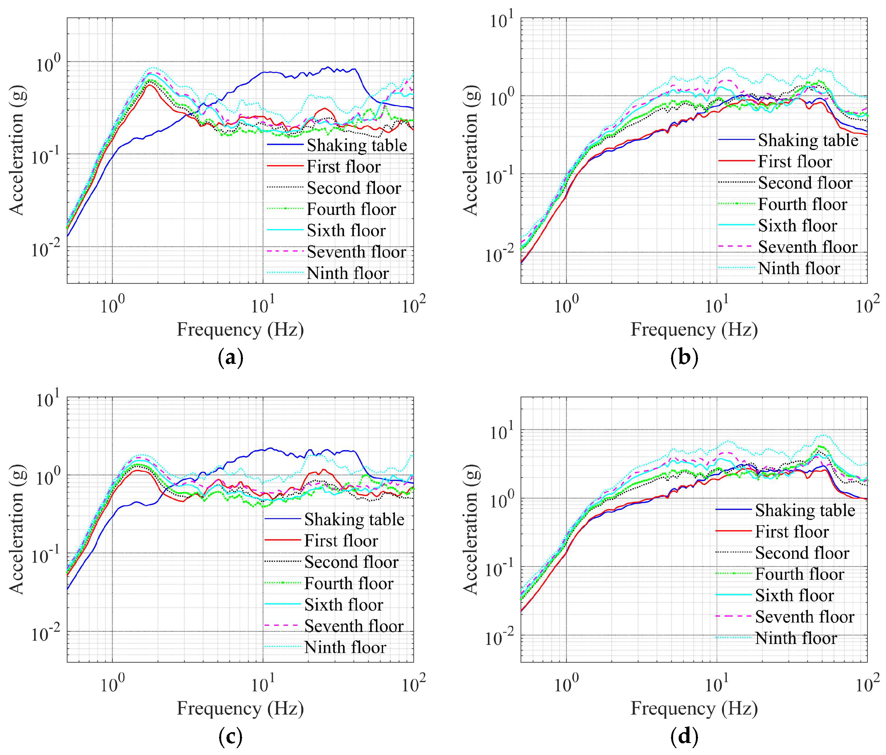
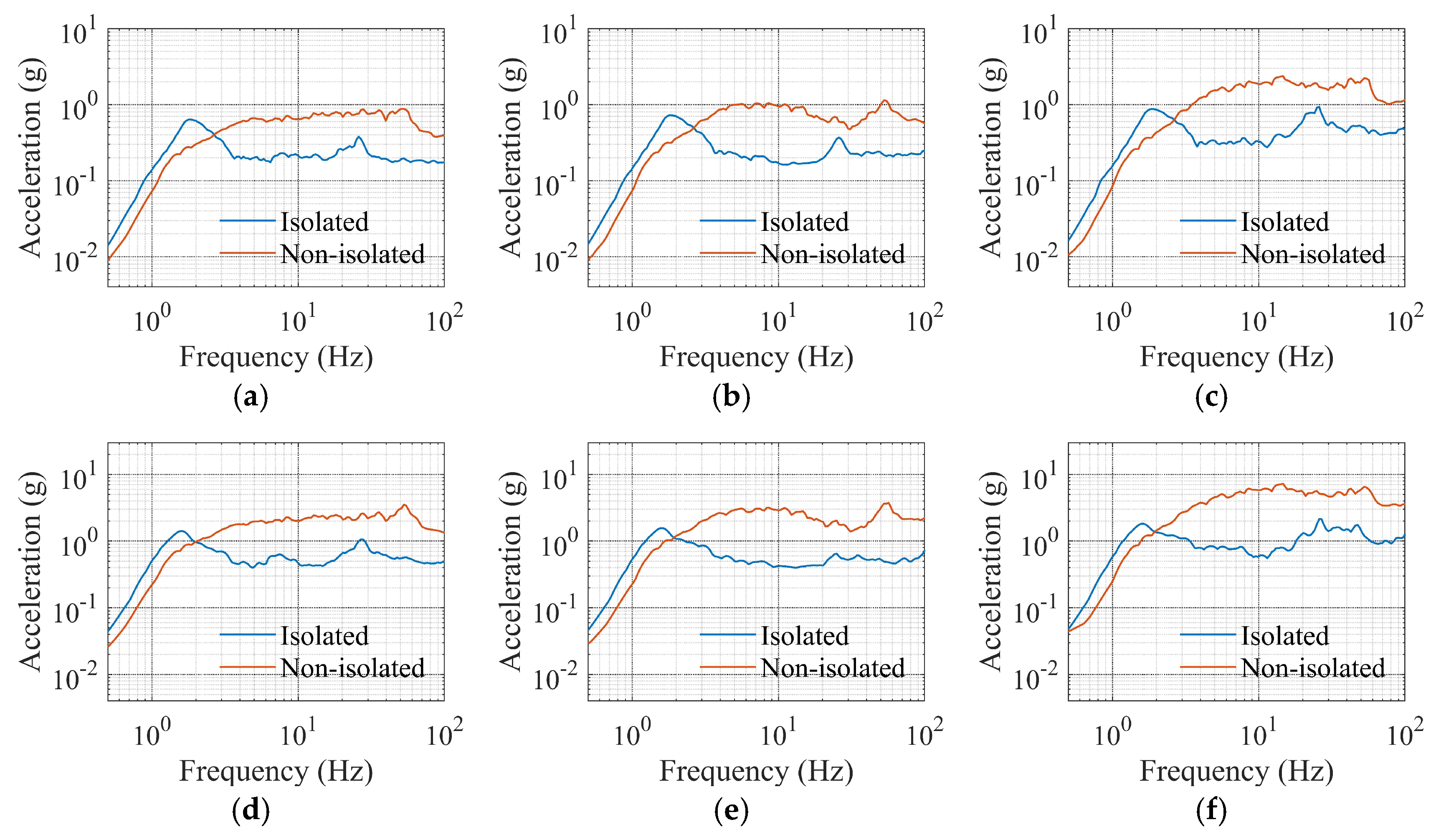
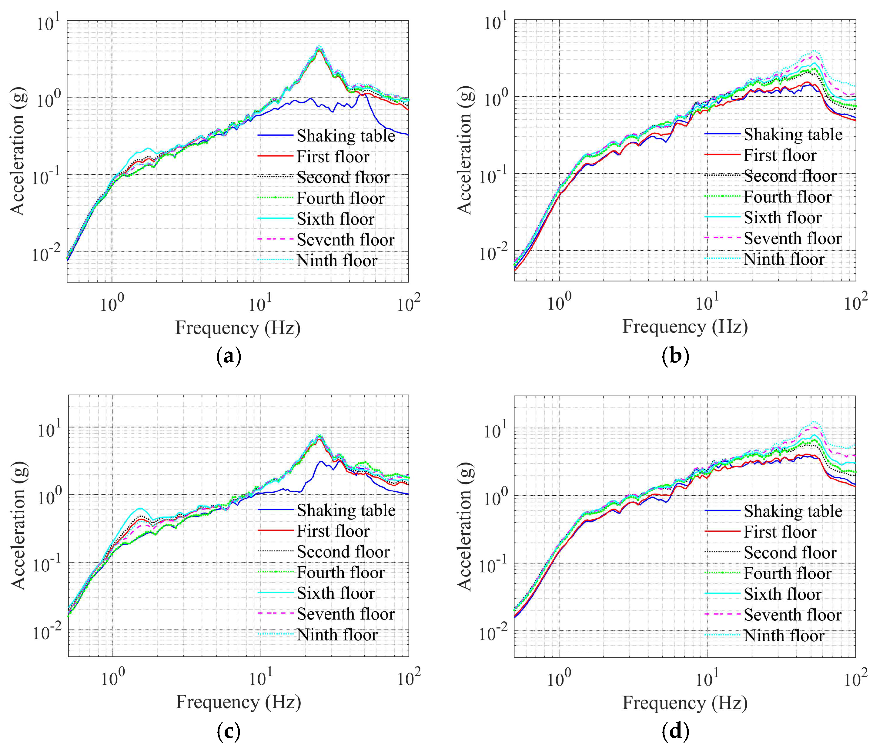
• Under tri-directional SL-1/SL-2 inputs, the isolated structure’s horizontal floor spectra exceed non-isolated counterparts below 3 Hz, while being suppressed above this threshold. Spectral reductions intensify with floor height and seismic intensity, and the predominant frequencies of the response spectrum effectively avoid the main operating frequencies of the equipment. Moreover, the predominant frequency of the vertical floor response spectrum is close to the vertical frequency of the isolation model, which is unfavorable for vertical isolation.
• Finite element simulations demonstrate alignment with experimental modal and dynamic responses, providing a reliable analysis method for further studies in the future.
• The equivalent horizontal stiffness of the LNR bearings and the nonlinear mechanical properties of the LRB bearings change with variations in compressive stress and shear strain, as confirmed by the comparative analysis of the finite element model results and experimental results and should be considered in the modeling process.
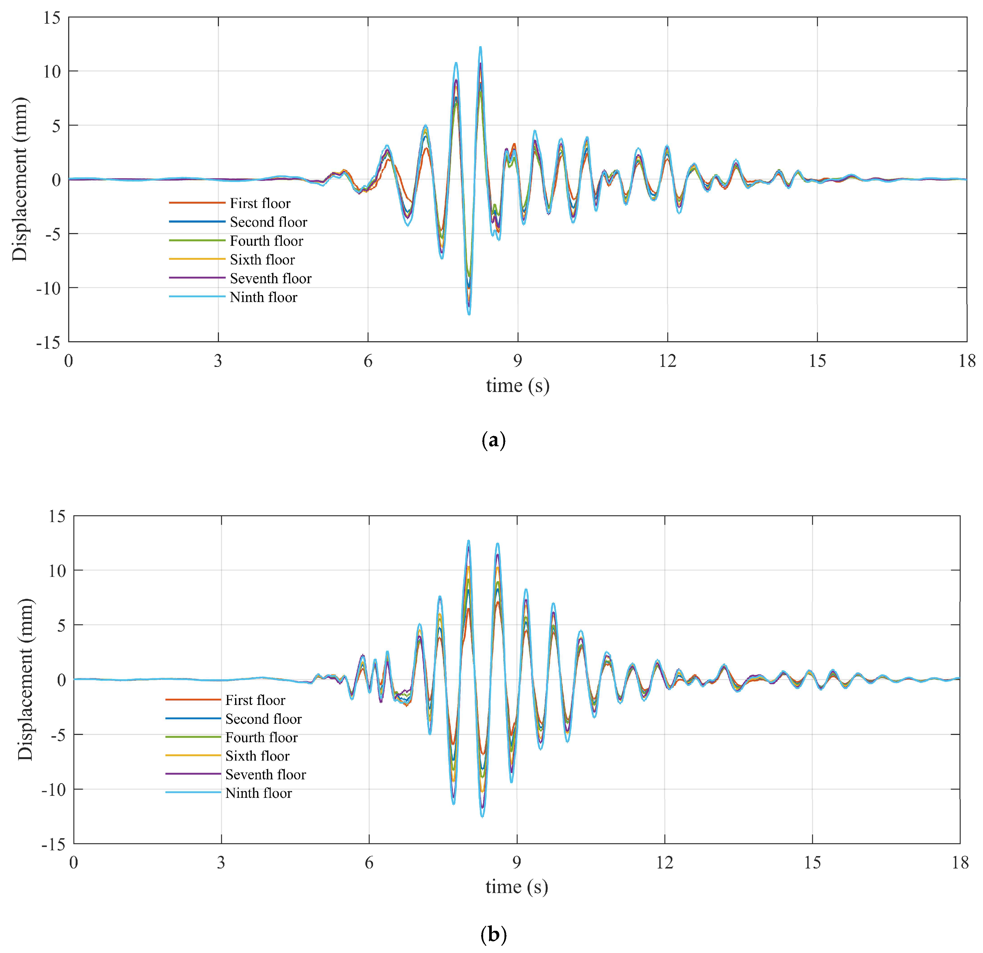
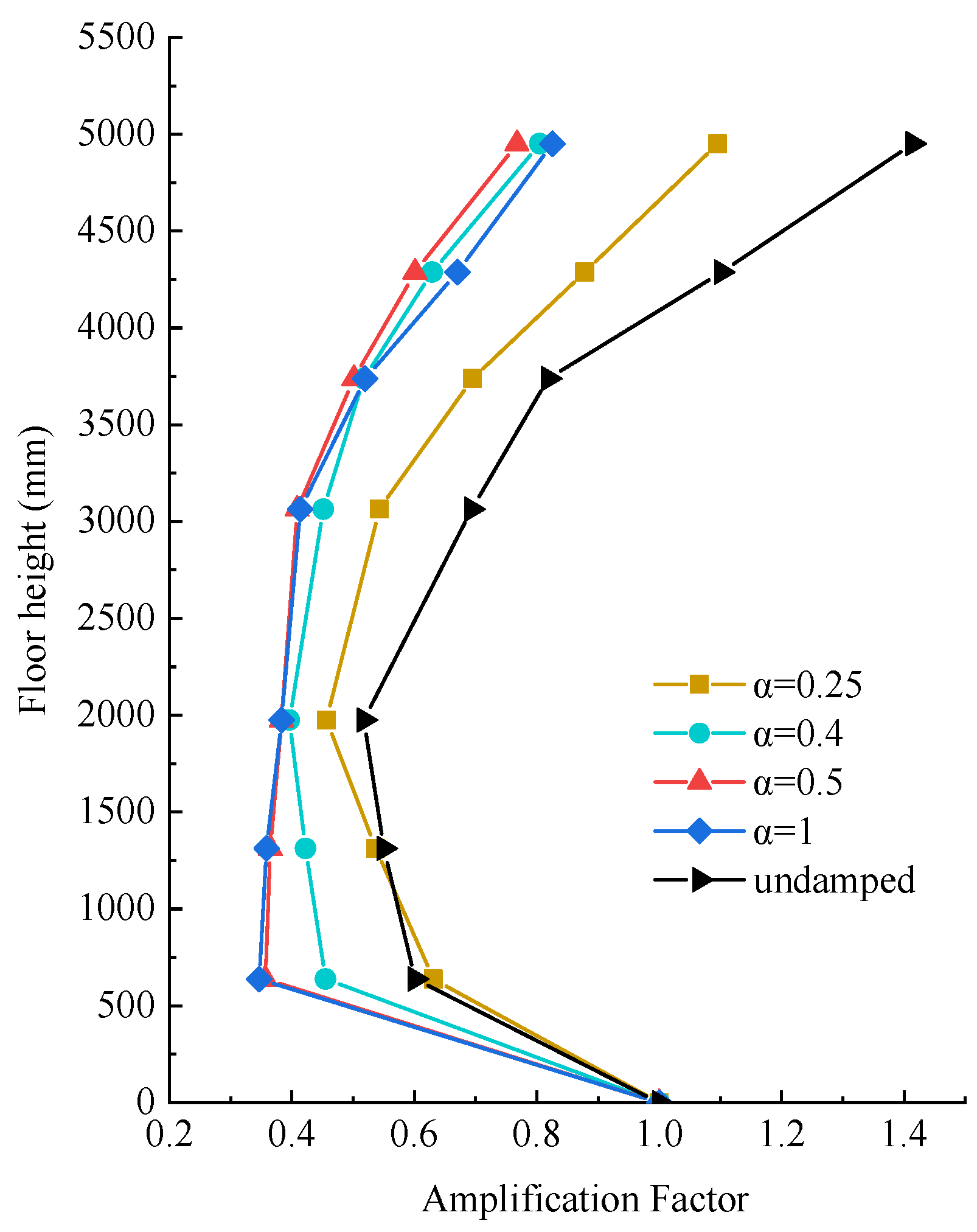
• The horizontal displacement of the isolation model primarily occurs in the isolation layer, with a certain overturning effect observed in the superstructure. Viscous dampers should be installed in the isolation layer to mitigate the overturning effect.
• Future studies will systematically investigate the coupling effects between diesel generators’ operational frequencies and artificial wave excitation through targeted numerical simulations and experimental campaigns, aiming to quantify their potential impacts on seismic isolation performance. Furthermore, the exploration of three-dimensional isolation techniques will be prioritized to mitigate overturning risks in base-isolated structures.

References

1. International Atomic Energy Agency (IAEA). Global Status of Nuclear Power Plants; IAEA: Vienna, Austria, 2021. [Google Scholar]
2. Nuclear Energy Agency (NEA). The Role of Nuclear Power in Mitigating Climate Change; OECD/NEA: Paris, France, 2020. [Google Scholar]
3. World Nuclear Association (WNA). Benefits of Nuclear Power; WNA: London, UK, 2023. [Google Scholar]
4. World Nuclear Association (WNA). Fukushima Daiichi Accident; WNA: London, UK, 2011. [Google Scholar]
5. Chan, R.W.K.; Lin, Y.S.; Tagawa, H. A smart mechatronic base isolation system using earthquake early warning. Soil Dyn. Earthq. Eng. 2019, 119, 299–307. [Google Scholar]
6. Xu, W.Z.; Du, D.S.; Wang, S.G.; Liu, W.Q.; Li, W.W. Shaking table tests on the multi-dimensional seismic response of long-span grid structure with base-isolation. Eng. Struct. 2019, 201, 109802. [Google Scholar]
7. Dicleli, M.; Karalar, M. Optimum characteristic properties of isolators with bilinear force-displacement hysteresis for seismic protection of bridges built on various site soils. Soil Dyn. Earthq. Eng. 2011, 31, 982–995. [Google Scholar]
8. Karalar, M.; Padgett, J.E.; Dicleli, M. Parametric analysis of optimum isolator properties for bridges susceptible to near-fault ground motions. Eng. Struct. 2012, 40, 276–287. [Google Scholar] [CrossRef]
9. Coladant, C. Seismic isolation of nuclear power plants—EDF’s philosophy. Nucl. Eng. Des. 1991, 127, 243–251. [Google Scholar] [CrossRef]
10. Chen, J.Y.; Zhao, C.F.; Xu, Q.; Yuan, C.Y. Seismic analysis and evaluation of the base isolation system in AP1000 NI under SSE loading. Nucl. Eng. Des. 2014, 278, 117–133. [Google Scholar]
11. Whittaker, A.S.; Kumar, M. Seismic Isolation of Nuclear Power Plants. Nucl. Eng. Technol. 2014, 46, 569–580. [Google Scholar]
12. Sarebanha, A.; Mosqueda, G.; Kim, M.K.; Kim, J.H. Seismic response of base isolated nuclear power plants considering impact to moat walls. Nucl. Eng. Des. 2018, 328, 58–72. [Google Scholar]
13. Zhao, C.F.; Yu, N.; Peng, T.; Lippolis, V.; Corona, A.; Mo, Y.L. Study on the dynamic behavior of isolated AP1000 NIB under mainshock-aftershock sequences. Prog. Nucl. Energy 2020, 119, 103144. [Google Scholar]
14. Kennedy, R.P.; Cornell, C.A.; Campbell, R.D.; Kaplan, S.; Perla, H.F. Probabilistic seismic safety study of an existing nuclear power plant. Nucl. Eng. Des. 1980, 59, 315–338. [Google Scholar] [CrossRef]
15. Lal, K.M.; Parsi, S.S.; Kosbab, B.D.; Ingersoll, E.D.; Charkas, H.; Whittaker, A.S. Towards standardized advanced nuclear reactors: Seismic isolation and the impact of the earthquake load case. Nucl. Eng. Des. 2021, 386, 111487. [Google Scholar] [CrossRef]
16. Firoozabad, E.S.; Jeon, B.G.; Choi, H.S.; Kim, N.S. Seismic fragility analysis of seismically isolated nuclear power plants piping system. Nucl. Eng. Des. 2015, 284, 264–279. [Google Scholar] [CrossRef]
17. Eidinger, J.M.; Kelly, J.M. Seismic isolation for nuclear power plants: Technical and non-technical aspects in decision making. Nucl. Eng. Des. 1985, 84, 383–409. [Google Scholar] [CrossRef]
18. Zheng, G.Y.; Peng, X.K.; Li, X.Z.; Kang, Y.X.; Zhao, X.G. Research on the standardization strategy of China’s nuclear industry. Energy Policy 2021, 155, 112314. [Google Scholar]
19. Parsi, S.S.; Lal, K.M.; Kosbab, B.D.; Ingersoll, E.D.; Shirvan, K.; Whittaker, A.S. Seismic isolation: A pathway to standardized advanced nuclear reactors. Nucl. Eng. Des. 2022, 387, 11445.1–111445.15. [Google Scholar] [CrossRef]
20. Warn, G.P.; Ryan, K.L. A Review of Seismic Isolation for Buildings: Historical Development and Research Needs. Buildings 2012, 2, 300–325. [Google Scholar] [CrossRef]
21. Sato, N.; Kato, A.; Fukushima, Y.; Iizuka, M. Shaking table tests on failure characteristics of base isolation system for a DFBR plant. Nucl. Eng. Des. 2002, 212, 293–305. [Google Scholar] [CrossRef]
22. Kim, M.K.; Choi, I.K.; Seo, J.M. A shaking table test for an evaluation of seismic behavior of 480 V MCC. Nucl. Eng. Des. 2012, 243, 341–355. [Google Scholar] [CrossRef]
23. Huang, B.F.; Lu, W.S.; Mosalam, K.M. Shaking Table Tests of the Cable Tray System in Nuclear Power Plants. J. Perform. Constr. Facil. 2017, 31, 04017018. [Google Scholar] [CrossRef]
24. Huang, Y.J.; Lu, D.G.; Liu, Y.; Zheng, S. Shaking table experiments on 3/10 reduced-scale CAP1400 spent fuel storage rack considering the effect of fluid-structure interaction. Nucl. Eng. Des. 2020, 369, 110861. [Google Scholar]
25. Jung, J.W.; Kim, M.K.; Kim, J.H. Experimental study on the floor responses of a base-isolated frame structure via shaking table tests. Eng. Struct. 2022, 253, 113763. [Google Scholar]
26. Micheli, I.; Cardini, S.; Colaiuda, A.; Turroni, P. A sensitivity investigation upon the dynamic structural response of a nuclear plant on aseismic isolating devices. Nucl. Eng. Des. 2004, 228, 319–343. [Google Scholar]
27. Zhao, C.F.; Chen, J.Y. Numerical simulation and investigation of the base isolated NPPC building under three-directional seismic loading. Nucl. Eng. Des. 2013, 265, 484–496. [Google Scholar]
28. Zhou, Z.G.; Wong, J.; Mahin, S. Potentiality of Using Vertical and Three-Dimensional Isolation Systems in Nuclear Structures. Nucl. Eng. Technol. 2016, 48, 1237–1251. [Google Scholar] [CrossRef]
29. Lim, H.G.; Yang, J.E.; Hwang, M.J. A quantitative analysis of a risk impact due to a starting time extension of the emergency diesel generator in optimized power reactor-1000. Reliab. Eng. Syst. Saf. 2007, 92, 961–970. [Google Scholar]