Triple-Layer Genetic Algorithm (3LGA) for Project Scheduling and Material Ordering Problem with Limited Storage Space

Abstract

Efficient project management in the construction industry depends on optimizing project scheduling and material ordering, two interdependent processes that significantly impact both costs and durations. Traditional approaches often address these processes separately, neglecting the trade-offs between scheduling costs and material procurement costs. Furthermore, existing studies frequently overlook real-world constraints, such as limited storage space at construction sites. To bridge these gaps, this paper investigates the project scheduling and material ordering problem with limited storage space (PSMOP-LSS) and introduces an integrated model that simultaneously optimizes storage space allocation, activity scheduling, and material ordering. A novel ordering strategy with time period (OSTP) is employed to enhance material procurement under storage constraints. To solve this NP-hard problem, a triple-layer genetic algorithm (3LGA) is proposed, comprising three layers: space allocation, project scheduling, and material ordering. Computational experiments conducted on a case study demonstrate the effectiveness of the 3LGA, achieving significant reductions in project costs and durations compared to conventional ordering strategies. The results highlight trade-offs between cost and duration, offering actionable insights for project managers. This research provides a robust decision-making framework for balancing inventory costs, ordering costs, and project durations in space-constrained environments. Managerial implications include optimizing ordering strategies based on storage capacity and cost parameters.

1. Introduction

The construction industry is a highly complex and dynamic field that requires careful planning and optimization to ensure efficient and cost-effective project execution [1]. Efficient project management in the construction industry hinges on optimizing project scheduling and material ordering. Project scheduling and material ordering are inherently interconnected, as the scheduling of project activities directly informs the material procurement process. Conversely, the delivery time and availability of materials exert a significant influence on the execution of scheduled activities [2,3]. Despite this evident interdependence, the project scheduling problem (PSP) and the material ordering problem (MOP) have traditionally been addressed as distinct areas of inquiry within the existing literature [4,5,6,7,8]. In conventional practice, a project schedule is typically formulated first, followed by the development of a material procurement plan based on the predetermined schedule. This sequential approach, however, neglects the potential trade-offs between the costs associated with scheduling (indirect cost and penalty/bonus cost) and those related to material procurement (ordering cost and inventory cost), thereby impeding the achievement of optimal cost efficiency [9,10]. The project scheduling and material ordering problem (PSMOP) has seen significant development since its introduction by Alfieri et al. [11]. They established an integrated scheduling model that combined the Critical Path Method (CPM) with Material Requirements Planning (MRP), laying the groundwork for future research. Building on this foundation, Mahdieh Akhbari advanced the PSMOP by developing mixed binary integer mathematical programming for practical projects that manage both materials and renewable resources simultaneously [12]. This marked the beginning of a broader exploration into the PSMOP, with researchers expanding the model’s applicability from various perspectives. A key advancement in PSMOP research was made by Tabrizi et al., who introduced a model constrained by capital limitations [13]. This model aimed to maximize net present value, addressing the financial constraints commonly encountered in real-world projects. In a different approach, Habibi et al. proposed the multi-project scheduling and material ordering problem (MPSMOP) through a tri-objective optimization model that balances economic, environmental, and quality factors [14]. By integrating supplier environmental assessments, quality evaluations, and advanced metaheuristic algorithms, the proposed approach enhances decision-making in complex construction projects. Recent advancements have further refined the PSMOP by integrating it with related problems. For example, Patoghi et al. and Zoraghi et al. explored the multi-mode resource-constrained project scheduling problem (MRCPSP) combined with material batch ordering, using metaheuristic methods to address these complex scenarios [15,16]. Kazemi et al. extended the PSMOP by incorporating variable execution intensities, presenting a mixed-integer programming model designed to minimize both makespan and cost [17]. Additionally, Dixit et al. introduced the concept of learning effects into the PSMOP framework, focusing on productivity gains derived from learning curves [18]. Tabrizi et al. and Zoraghi et al. tackled uncertainties in activity durations by developing a bi-objective model to balance cost minimization with robustness, where robustness was measured using free slacks [19,20]. Zhang et al. also contributed by devising a two-stage heuristic method to handle PSMOP with uncertain activity durations [21]. Further research by Yeo et al. and Lu et al. examined procurement uncertainties within the PSMOP framework [22,23].

Recent research on the project scheduling and material optimization problem (PSMOP) has broadened its focus by incorporating supplier selection as a key factor. In this extended version of the PSMOP, scholars address not only scheduling activities and developing material ordering schemes but also the simultaneous selection of appropriate material suppliers. Tabrizi et al. were among the first to introduce this variant, emphasizing the importance of supplier selection alongside traditional project scheduling [19]. Beyond operational concerns, environmental considerations have also been integrated into the supplier selection process. Tabrizi et al. and Habibi et al. extended the PSMOP by including environmental factors, proposing a multi-objective programming model that addresses both cost-efficiency and sustainability in material procurement [24,25]. This model was solved using the NSGA-II algorithm. Further efforts to optimize the PSMOP with supplier selection have focused on maximizing the net present value (NPV). Tabrizi et al. and Asadujjaman et al. developed models that integrate supplier selection with project scheduling to improve financial outcomes [26,27]. These models, solved using meta-heuristic approaches, provided effective solutions to the complex challenges of scheduling and material procurement.

Effective project scheduling and material ordering play a crucial role in ensuring the timely and cost-effective execution of construction projects. These two factors directly impact project duration, cost control, and resource utilization. However, real-world construction projects frequently face limited storage space, which significantly affects material delivery, storage management, and construction sequencing. This issue is particularly critical in urban high-rise buildings, highway infrastructure, and subway tunnel construction, where storage constraints result from restricted land availability, safety regulations, and logistical challenges. In high-density urban projects, available on-site storage is often highly restricted due to adjacent structures, active roadways, or underground utilities. Subway station construction must manage material deliveries within strict spatial constraints, preventing bulk material storage. Bridge and highway projects require efficiently staged material deliveries, as roadside storage is typically unavailable. To address storage constraints, many construction projects adopt just-in-time (JIT) procurement, ensuring that materials are delivered precisely when needed, rather than being stored on-site for extended periods. Large-scale infrastructure projects, such as tunnel boring machine (TBM) operations, rely on JIT strategies to deliver precast segments, steel reinforcements, and cement in a phased manner. Improper procurement scheduling under storage constraints can lead to project delays, material shortages, or excessive handling costs.

While significant progress has been made in the study of the project scheduling and material optimization problem (PSMOP), the issue of space constraints has remained relatively underexplored. Sha et al. were among the first to address this gap by investigating the PSMOP with space constraints [28]. However, their study assumed that the storage space required for each material was predetermined, overlooking the practical challenges of spatial competition among materials. In real-world construction projects, allocating storage space is a crucial early task for project managers, especially when the total available site space is limited. Designing an efficient storage plan for various materials is essential to avoid bottlenecks and disruptions during the construction process. However, existing research, including Zhang et al.’s study, does not fully account for the complexities of dynamically managing limited storage space while addressing the competing needs of different materials [3]. This gap highlights the need for further research into optimizing storage space in PSMOP models, where spatial competition and constraints play a key role in project success. Consequently, the integration of project scheduling and the material ordering plan is essential to minimize total project costs, particularly in scenarios where storage space is constrained. This issue becomes particularly critical for projects facing limited storage space, a common constraint in urban environments and other congested areas where land and storage facilities are scarce [29,30,31]. Managing limited storage space for materials with varying requirements is a critical challenge in construction projects. The improper allocation of storage can result in material damage, delays, and increased costs. Traditional methods often overlook the specific needs of different materials and the dynamic nature of construction, emphasizing the need for more advanced strategies. Limited storage space complicates material deliveries: early deliveries may overcrowd storage areas, while late deliveries can cause project delays. Additionally, managing multiple suppliers adds complexity to material handling. Therefore, advanced optimization techniques are essential to integrate storage allocation, material ordering, and scheduling, ensuring that storage constraints do not disrupt project progress.

In project scheduling and material ordering problems (PSMOPs), selecting the right ordering strategy is essential for optimizing project performance. Two main strategies are commonly discussed: the ordering strategy based on the time period (OSTP) and the ordering strategy based on the activity (OSA). The OSTP involves ordering materials incrementally based on specific time period needs, reducing upfront storage and providing flexibility, which can result in cost savings, particularly when material demand varies [32,33]. In contrast, the OSA requires all materials for an activity to be procured in a single order before the activity begins [3,34]. While this ensures uninterrupted work, it increases storage demands. This makes the OSA inefficient for projects with limited storage capacity, as it requires all materials to be stored in advance. For example, if an activity requires 12 units of material over 3 days, the OSA mandates that all 12 units be stored beforehand, whereas the OSTP allows 4 units to be ordered daily, reducing storage requirements. The OSTP’s flexibility is particularly beneficial for projects with limited storage, as it helps minimize idle inventory and reduce costs. Thus, the OSTP is often more suitable for projects with space and cost constraints, offering key advantages in storage efficiency and cost reduction.

The project scheduling and material ordering problem (PSMOP) has garnered considerable academic attention due to its crucial role in optimizing project performance. However, significant gaps remain in the literature, particularly regarding the management of limited storage space for multiple materials at construction sites. Existing studies often assume either unlimited or predetermined inventory capacity, which does not accurately reflect real-world constraints, such as those encountered in highway or subway projects. Additionally, the widely used ordering strategy based on activity (OSA) is inadequate for projects with storage limitations.

To address these issues, this study investigates the project scheduling and material ordering problem with limited storage space (PSMOP-LSS) and introduces a novel ordering strategy based on time period (OSTP) to optimize storage utilization.

The research gaps and key contributions of this paper are as follows:

• Integrated model
  • Introduces the PSMOP-LSS, which integrates project scheduling, material ordering, and storage allocation into a unified approach;
  • Utilizes the OSTP strategy to enhance storage efficiency, overcoming the limitations of the traditional OSA approach.
• Efficient solution approach
  • Develops a triple-layer genetic algorithm (3LGA) to solve the NP-hard (a classification of computational problems for which no known algorithm can solve all instances efficiently in polynomial time) PSMOP-LSS.
  • The 3LGA consists of three layers:

    ∘

    Space allocation (SA) layer;

    ∘

    Project scheduling (PS) layer;

    ∘

    Material ordering (MO) layer.

  • This approach provides an effective and scalable solution for projects with storage constraints.
• Practical insights
  • Provides valuable guidance for project managers working in space-constrained environments;
  • Enables informed decision-making to reduce costs and improve project efficiency.
• Computational validation
  • Conducts extensive computational experiments and sensitivity analyses to validate the model and algorithm;
  • Ensures the robustness and practical applicability of the proposed approach.

2. Problem Definition

In construction projects, the timely and efficient management of materials is essential due to the complex interdependencies between project scheduling and material ordering. Limited storage space introduces significant challenges, as it affects both the frequency of material orders and the ability to execute multiple activities simultaneously. This necessitates careful planning to balance material availability with storage constraints. The project scheduling and material ordering problem with limited storage space (PSMOP-LSS) addresses these challenges by integrating material ordering decisions with project scheduling. The primary goal of the PSMOP-LSS is to ensure that materials are ordered, delivered, and stored in alignment with the demands of project activities while accommodating limited storage capacity. Specifically, project managers must decide the appropriate storage size for each material, when to initiate each activity, when to place material orders, and how much material to order in each period.

The project network in the PSMOP-LSS is represented using an activity-on-node (AON) graph G = (V, E) where V represents the set of all activities, and E denotes the immediate precedence relationships between them. The project starts with dummy activity 1 and ends with dummy activity I. Both activities have zero duration and do not consume any resources. Each activity requires a set of renewable resources and materials for execution. In this study, it is assumed that renewable resources are always available throughout the project, while materials must be ordered and stored before use. Moreover, no activity can proceed without the necessary materials, and material shortages are not permitted.

Given the fixed storage capacity for all materials, the ordering strategy based on the time period (OSTP) is implemented to guide the material ordering process. The following assumptions, based on previous studies, are made: 1. The ordering process for different materials is independent of one another. 2. The ordering cost is fixed regardless of the quantity of materials purchased. 3. Materials arrive at the construction site at the beginning of each period. 4. Storing materials in storage incurs inventory costs at the end of each period.

The PSMOP-LSS, as defined in this paper, aims to minimize the project cost and/or the project duration by simultaneously optimizing three variables: the schedule of all project activities, the storage space allocated for each material, and the quantity of materials ordered in each period. By integrating these variables, the formulation seeks to ensure efficient project execution within the constraints of limited storage space and material availability.

3. Notations and Objective Functions

The notations used in the concurrent project scheduling and material ordering problem under limited storage space (PSMOP-LSS) model are defined in

Table 1. Definitions of notations.

Notations	Description
Indices
$i=1, 2, \dots , I$	Index of activities.
$m=1, 2, \dots , M$	Index of materials.
$t=1, 2, \dots , T$	Index of period.
Sets
$V$	Set of activities.
$E$	Set of immediate precedence relationships.
$A_{\left(t\right)}$	Set of eligible activities at period t.
$P_{\left(i\right)}$	Set of immediate predecessors of activity i.
$S_{\left(i\right)}$	Set of immediate successors of activity i.
Parameters
$d_{\left(i\right)}$	Duration of activity i.
$R_{\left(i, m\right)}$	Quantity of material m required by activity i
S	Total storage space of materials at the project site.
$v_{\left(m\right)}$	Size of storage space of material m per unit capacity.
${OC}_{\left(m\right)}$	Cost of placing an order of material m.
${IC}_{\left(m\right)}$	Cost per unit of storing material m per unit.
$C_I$	Indirect cost per unit period.
T	Planning horizon.
${ES}_{\left(i\right)}$	Early start time of activity i.
${EF}_{\left(i\right)}$	Early finish of activity i.
${LS}_{\left(i\right)}$	Late start time of activity i.
${LF}_{\left(i\right)}$	Late finish time of activity i.
${TF}_{\left(i\right)}$	Total float of activity i.
$x_{\left(i, t\right)}$	A binary variable that equals 1 if activity i proceeds during period t.
PD	Project Duration
PC	Project Cost
Intermediate Variables
${\sigma }_{\left(i\right)}$	Activity list
$r_{\left(i,m\right)}$	Quantity of material m required by activity i per unit period.
${MR}_{\left(m, t\right)}$	Quantity of material m required at period t.
${TMR}_{\left(m\right)}$	Total quantity of material m required for the entire project.
$c_{\left(m\right)}$	Storage capacity of material m.
$s_{\left(m\right)}^{min}$	Lower bound of the storage space for material m.
$s_{\left(m\right)}^{max}$	Upper bound of the storage space for material m.
${LQ}_{\left(m, t\right)}$	Lower bound on the quantity of material m ordered at the beginning of period t.
${UQ}_{\left(m, t\right)}$	Upper bound on the quantity of material m ordered at the beginning of period t.
${IB}_{\left(m, t\right)}$	Inventory quantity of material m at the beginning of period t.
${IE}_{\left(m, t\right)}$	Inventory quantity of material m at the end of period t.
${\beta }_{\left(m, t\right)}$	A binary auxiliary variable that equals 1 if material m is ordered at period t or 0 otherwise.
${SF}_{\left(m, t\right)}$	Sufficient factor.
${BF}_{\left(m, t\right)}$	Balance factor.
Decision Variable
${\delta }_{\left(i\right)}$	Delay period of activity i later than its early start time.
$s_{\left(m\right)}$	Storage space of material m.
$q_{\left(m, t\right)}$	Quantity of material m ordered at the beginning of period t.

.

The bi-objectives of the PSMOP-LSS mode are proposed to simultaneously minimize project duration (min PD) and total project cost (min PC). These two objective functions of the model are presented in Equations (1) and (2), respectively. The first objective aims to minimize the project duration, as in Equation (1). The second objective seeks to minimize project costs, which include the ordering costs, the inventory costs, and the indirect costs, as in Equation (2).

$$min PD=\underset{i\in V}{max} {EF}_{\left(i\right)}$$

(1)

$$min PC=\sum _{m=1}^M\sum _{t=1}^T\left({\beta }_{\left(m, t\right)}·{OC}_{\left(m\right)}+{IE}_{\left(m, t\right)}{·IC}_{\left(m\right)}\right)+PD·C_I$$

(2)

4. Triple-Layer Genetic Algorithm (3LGA)

The project scheduling and material ordering problem with limited storage space (PSMOP-LSS) is a complex, NP-hard optimization problem (a classification of computational problems for which no known algorithm can solve all instances efficiently in polynomial time) involving multiple interdependent decisions, including task sequencing, material procurement, and storage allocation. Solving this problem efficiently is crucial for minimizing project delays, cost overruns, and material handling inefficiencies.

Among various optimization approaches, genetic algorithms (GAs) offer significant advantages over other metaheuristics and mixed-integer programming (MIP) methods due to their ability to handle large-scale, combinatorial, and multi-objective problems. Below are the key reasons why GAs are the best choice for addressing PSMOP-LSS:

• Scalability and computational efficiency
  • MIP limitation: mixed-integer programming (MIP) methods often struggle with large-scale problems due to their exponential complexity, making them impractical for real-world construction projects.
  • GA advantage: GAs use population-based search and parallel processing, allowing them to efficiently explore large solution spaces without requiring explicit mathematical formulations.
• Ability to handle multi-objective optimization
  • PSMOP-LSS complexity: the problem involves conflicting objectives, such as minimizing project duration, reducing material ordering costs, and optimizing storage utilization.
  • GA strength: unlike traditional optimization approaches that require complex weighting schemes, GAs naturally handle multi-objective trade-offs by maintaining a diverse set of solutions.
• Adaptability to real-world constraints
  • MIP limitation: MIP requires strict linear or integer constraints, which may not accurately model dynamic storage space variations, uncertain deliveries, and changing construction schedules.
  • GA advantage: GAs can integrate adaptive constraints, such as dynamic storage availability, uncertainty in procurement schedules, and just-in-time (JIT) delivery policies, making them more flexible for real-world applications.
• Effective exploration and exploitation of the solution space
  • Metaheuristic comparison: other metaheuristic algorithms, such as simulated annealing (SA) and tabu search (TS), often focus on exploitation (intensification), leading to premature convergence to local optima.
  • GA strength: GAs balance exploration (diversity) and exploitation (selection of optimal solutions) through mechanisms like mutation, crossover, and selection, ensuring a higher probability of finding near-optimal solutions.
• Customizability and hybridization
  • PSMOP-LSS complexity: the problem requires integrating project scheduling, material ordering, and storage allocation, each with unique constraints.
  • GA advantage: GAs allow for customized encoding (e.g., chromosome representation for task sequencing, material ordering schedules, and storage allocations) and can be hybridized with problem-specific heuristics to improve performance.
• Robustness against uncertainty and dynamic conditions
  • Real-world challenges: construction projects face uncertain delays, fluctuating material costs, and space constraints that evolve over time.
  • GA strength: GAs is well suited for handling dynamic environments by adapting mutation rates and selection strategies to optimize solutions as project conditions change.

Given the NP-hard nature (a classification of computational problems for which no known algorithm can solve all instances efficiently in polynomial time) of the PSMOP-LSS, the flexibility, scalability, and multi-objective capabilities of genetic algorithms make them superior to traditional MIP approaches and other metaheuristics. Their ability to integrate adaptive constraints, handle uncertainty, and optimize large-scale project scheduling problems ensures their effectiveness in addressing complex, real-world construction challenges. Therefore, this study applies a genetic algorithm approach to obtain the optimal solution for the PSMOP-LSS model.

The NP-hardness of PSMOP-LSS, along with the interdependencies among the decision variables (${\delta }_{\left(i\right)}, s_{\left(m\right)} \mathrm{and} q_{\left(m, t\right)}$), makes this problem more complex. The PSMOP-LSS can be decomposed into three interconnected subproblem layers: the space allocation layer (SA), the project scheduling layer (PS), and the material ordering layer (MO). First, the value of $s_{\left(m\right)}$ is determined in the SA layer, and the value of ${\delta }_{\left(I\right)}$ is determined in the PS layer, enabling the required capacity for each material to be calculated. The results from the SA and PS layers are then used to determine $q_{\left(m, t\right)}$ in the MO layer. This subsection describes the decomposition approach for the PSMOP-LSS.

4.1. Space Allocation Layer (SA)

Equation (3) represents the relationship between the storage capacity of a material and the storage space it requires per unit of capacity. Equation (4) states that the total space consumed by all materials in the storage must not exceed the available storage space on the construction site. Since the materials consumed per period must be stored in advance, the storage capacity of each material ($c_{\left(m\right)}$) must be at least equal to the quantity of material required by each activity per unit period ($r_I$). Therefore, the lower bound of the storage space for each material can be calculated as shown in Equation (5). Meanwhile, when the storage space of other materials is $s_{\left(k\right)}^{min}\left(kϵM\setminus \left\{m\right\}\right)$ and the remaining space is allocated to material m, the storage space for material m reaches its upper bound, as shown in Equation (6).

$$c_{\left(m\right)}=s_{\left(m\right)}/v_{\left(m\right)}, \left(c_{\left(m\right)}, s_{\left(m\right)}, v_{\left(m\right)}\right)\in \mathbb{R}$$

(3)

$$\sum _{m = 1}^M{s}_{\left(m\right)} \le S$$

(4)

$$s_{\left(m\right)}^{min}=\underset{i\in V}{max}\left\{r_{\left(i, m\right)}\right\}· v_{\left(m\right)}$$

(5)

$$s_{\left(m\right)}^{max}=S-\sum _{kϵM\setminus \left\{m\right\}}{s}_{\left(k\right)}^{min}$$

(6)

The chromosome representation of the space allocation, which consists of the space allocation list $s_{\left(m\right)}$, represents the space allocation plan. The list $s_{\left(m\right)}$ = ($s_{\left(1\right)}, \dots ,s_{\left(M\right)}$) contains real numbers that define the storage space for each material. Based on the lower and upper bounds of $s_{\left(m\right)}$, as shown in Equations (5) and (6), the feasible domain of $s_{\left(m\right)},\left(m\in M\right)$ is $\left(s_{\left(m\right)}^{min},s_{\left(m\right)}^{max}\right)$, ensuring that all chromosomes are feasible under the storage space constraint. Figure 1 illustrates an example of the chromosome representation in the space allocation layer for three materials, assuming that the total storage space for materials at the project site is 54 units.

4.2. Project Scheduling Layer (PS)

To perform project scheduling based on critical path analysis transparently, we model it using the precedence relationships as in Equations (7)–(13). The delay period of each activity, defined as the time beyond its early start, is introduced as a decision variable. Initially, the delay period for each activity can be set to zero. These delay values allow adjustments to the schedule to ensure that the material requirements of each period are met with the available material at the beginning of that period.

Considering these delays, the forward pass calculation determines the early start of each activity. An activity can start only after the latest of those predecessors has finished and its delay period has passed, as shown in Equation (7). The early finish of the activity is calculated as its early start plus its duration, as defined in Equation (8). Conversely, the backward pass calculation determines the late finish of each activity. The last activity, which has no successors, is assigned a late start equal to the planning horizon, as described in Equation (9). The planning horizon is assumed to be the sum of all activity durations. An activity must finish no later than the earliest late start of its successors, as outlined in Equation (10). The late start of an activity is calculated as its late finish minus its duration, as shown in Equation (11). The total float of an activity, as defined in Equation (12), represents the amount of time an activity can be delayed from its early start without affecting the planning horizon. Additionally, constraints defined in Equation (13) ensure that an activity proceeds only within the window between its early start and early finish.

$${ES}_{\left(i\right)}=\underset{j\in P_{\left(i\right)}}{max}\left({EF}_{\left(j\right)}+{\delta }_{\left(i\right)}\right)$$

(7)

$${EF}_{\left(i\right)}={ES}_{\left(i\right)}+d_{\left(i\right)}$$

(8)

$${LF}_{\left(I\right)}=T$$

(9)

$${LF}_{\left(i\right)}=\underset{j\in S_{\left(i\right)}}{min}\left({LS}_{\left(j\right)}-{\delta }_{\left(j\right)}\right)$$

(10)

$${LS}_{\left(i\right)}={LF}_{\left(i\right)}-d_{\left(i\right)}$$

(11)

$${TF}_{\left(i\right)}={LF}_{\left(i\right)}-{EF}_{\left(i\right)}$$

(12)

$${ES}_{\left(i\right)} < t·x_{\left(i, t\right)} \le {EF}_{\left(i\right)}$$

(13)

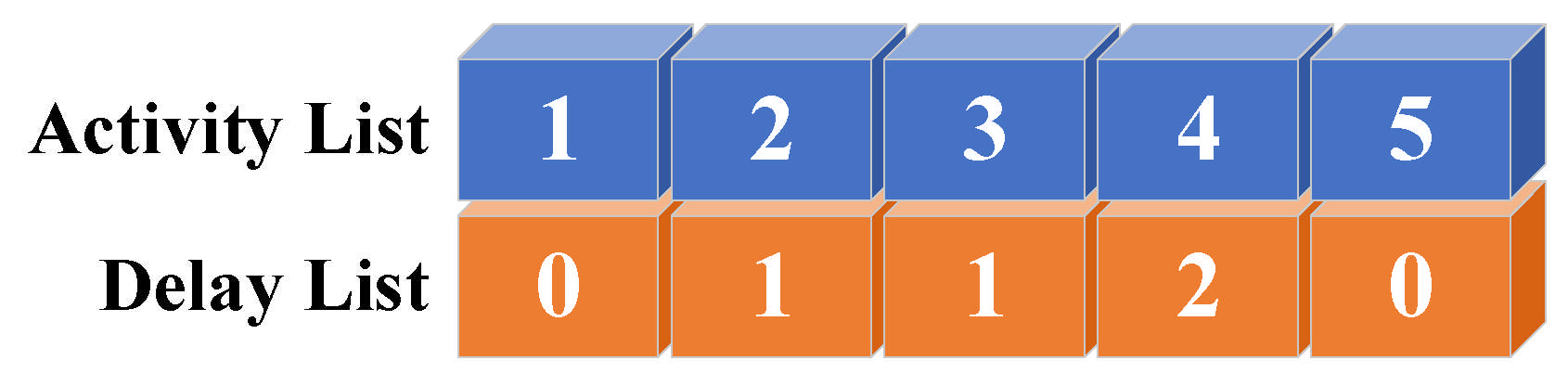
An appropriate solution representation plays a significant role in genetic algorithms (GAs). Therefore, a two-list chromosome representation is proposed to encode the solutions for project scheduling, as illustrated in Figure 2 The first row represents the activity list, and the second row represents the delay list.

4.3. Material Ordering Layer (MO)

This subsection presents a detailed algorithm designed to determine the optimal material ordering for individual materials, based on the space allocation plan and the demanding profiles.

When ${\delta }_{\left(i\right)}$ and $s_{\left(m\right)}$ are fixed, the material consumption per unit period for an activity is assumed to be equal to the total material required by the activity, evenly distributed over its duration, as shown in Equation (14). For any unit period under consideration, the material needs are calculated by summing the requirements for that material across all active activities during the period, as described in Equation (15). The total material requirement for the entire project can be calculated by summing the requirements across all activities, as shown in Equation (16).

$$r_{\left(i, m\right)}=R_{\left(i, m\right)}/d_{\left(i\right)}$$

(14)

$${MR}_{\left(m, t\right)}=\sum _{i=1}^I{r}_{\left(i, m\right)}· x_{\left(i, t\right)}$$

(15)

$${TMR}_{\left(m\right)}=\sum _{i=1}^I{R}_{\left(i, m\right)}$$

(16)

Equations (17)–(21) represent the constraints related to material ordering. Equation (17) states that adding the ordered amount of material m in period t sets the inventory level at the beginning of period t equal to the level at the end of period t − 1. Similarly, deducting the quantity consumed during period t adjusts the inventory level accordingly. Equation (18) reiterates this relationship, emphasizing that the inventory at the beginning of period t is the sum of the inventory at the end of period t − 1 and the ordered amount for period t, minus the quantity consumed during period t. Equation (19) ensures that the inventory level of each material in every period does not exceed the storage capacity. Equation (20) shows that the inventory level at the end of period t is determined by subtracting the total material required by all activities in that period from the inventory at the beginning of the period. Finally, Equation (21) ensures that no material shortages occur.

$${IE}_{\left(m, 0\right)}=0$$

(17)

$${IB}_{\left(m, t\right)}={IE}_{\left(m, t-1\right)}+q_{\left(m, t\right)}$$

(18)

$${IB}_{\left(m, t\right)} \le c_{\left(m\right)}$$

(19)

$${IE}_{\left(m, t\right)}={IB}_{\left(m, t\right)}-{MR}_{\left(m, t\right)}$$

(20)

$${IE}_{\left(m, t\right)} \ge 0$$

(21)

The sufficient factor, as described in Equation (22), determines whether material must be ordered at the beginning of the current period, based on whether the remaining inventory at the end of the previous one-unit period is sufficient to meet the material requirement. If the inventory is insufficient, the sufficient factor takes a value of 1; otherwise, it takes a value of 0. The balance factor ensures that material is not ordered in excess of the total quantity required for the entire project. Specifically, if the accumulated ordered material up to the beginning of the previous one-unit period has not yet reached the total requirement for the entire project, the balance factor takes a value of 1; otherwise, it takes a value of 0, as described in Equation (23). Equation (24) introduces an auxiliary binary variable, which equals 1 if an order is placed in period t for material m and 0 otherwise. This auxiliary binary variable depends on the sufficient factor and the balance factor. When considering the auxiliary binary variable, the variable $\alpha$ will be a binary variable generated through randomization. If the inventory quantity of the material is sufficient to meet the material requirement and the accumulated ordered material is less than the total requirement for the entire project, ordering additional material is optional. However, additional material must be ordered if the inventory quantity of the material is insufficient to meet the material requirement. Conversely, no additional material should be ordered if the accumulated ordered material already satisfies the total requirement for the entire project.

$${SF}_{\left(m, t\right)}=\left\{\begin{array}{c}1,\hspace{1em}{IE}_{\left(m, t\right)}\ge {MR}_{\left(m, t\right)}\hfill \\ 0,\hspace{1em}otherwise\hfill \end{array}\right.$$

(22)

$${BF}_{\left(m, t\right)}=\left\{\begin{array}{c}1,\hspace{1em}{\displaystyle \sum _{\tau =1}^{t-1}}{q}_{\left(m, \tau \right)} <{TMR}_{\left(m\right)}\hfill \\ 0,\hspace{1em}otherwise\hfill \end{array}\right.$$

(23)

$${\beta }_{\left(m, t\right)}=\left[\left(\alpha -1\right)·{SF}_{\left(m, t\right)}+2{BF}_{\left(m, t\right)}- 1\right]·{BF}_{\left(m, t\right)}, \alpha \mathrm{ϵ}\left(0, 1\right)$$

(24)

Equation (25) defines the decision variables for material ordering, which are positive if an order for material m is placed at period t and equal to 0 if no order is placed. The material ordering quantity depends on an auxiliary binary variable, as described in Equation (24), and must fall between the lower and upper bound quantities, as specified in Equations (26) and (27), respectively. The lower bound of material ordering must not be less than the quantity of material in inventory at the end of the previous one-unit period that is still insufficient to meet the material requirement for the current period, and it must be 0 otherwise, as described in Equation (26). The upper bound of material ordering must not exceed the remaining quantity required to fulfill the total material requirement for the entire project or the remaining storage capacity, whichever is smaller, as described in Equation (27).

$$q_{\left(m, t\right)}={\beta }_{\left(m, t\right)}·X, X ~ U\left[\left({LQ}_{\left(m, t\right)}, {UQ}_{\left(m, t\right)}\right)\right]$$

(25)

$${LQ}_{\left(m, t\right)}=\left\{\begin{array}{cc}{MR}_{\left(m, t\right)}-{IE}_{\left(m, t-1\right)}\hfill & , {IE}_{\left(m, t-1\right)} < {MR}_{\left(m, t\right)}\hfill \\ 0\hfill & , otherwise\hfill \end{array}\right.$$

(26)

$${UQ}_{\left(m, t\right)}=min\left({TMR}_{\left(m\right)}-\sum _{\tau =1}^{t-1}{q}_{\left(m, \tau \right)}, c_{\left(m\right)}-{IE}_{\left(m, t-1\right)}\right)$$

(27)

The material ordering layer algorithm determines the optimal purchasing cost for a specific scheduling scheme by using the material requirements (${MR}_{\left(m, t\right)}$) as inputs. Consequently, the total cost for an individual is calculated as the sum of the indirect costs and the purchasing costs.

4.4. BI-Objective Optimization Search Using Genetic Algorithms

To address the bi-objectives described in Equations (1) and (2), a search technique based on artificial intelligence—genetic algorithms (Gas)—is employed. Gas, inspired by the principles of natural selection and genetics, have been successfully applied to solve numerous science and engineering problems. They have proven to be an efficient method for identifying optimal solutions in large problem domains, such as the one under consideration. At their core, Gas are optimization search procedures modeled after the biological process of evolution, in which systems improve their fitness over generations. They use a random yet directed search to locate the globally optimal solution. This approach typically requires a representation scheme to encode feasible solutions to the optimization problem, often in the form of strings called chromosomes (or genes). Each chromosome represents a potential solution and is evaluated based on its fitness, which is determined by an objective function. To simulate the natural “survival of the fittest” process, the fittest chromosomes exchange information to produce offspring. These offspring are then evaluated and retained only if they demonstrate superior fitness compared to others in the population. This process is repeated over multiple generations until an optimal solution (or gene) is identified. Implementing the GA technique for the current problem involved three primary steps: 1. generating the initial population of chromosomes, 2. evaluating the fitness value of each chromosome, and 3. applying crossover and mutation operations.

4.4.1. Generating Initial Population

Suppose the population size and the maximum number of generations for 3LGA are $P_{size}$ and $G_{max}$, respectively. To ensure feasibility and population quality, each individual in the initial population is generated using specific procedures. First, materials are arranged in descending order of $v_{\left(m\right)}$, meaning that for any $a<b,v_{\left(a\right)} >v_{\left(b\right)}$ holds. We assume that the set $M_1$ contains the materials already allocated storage space, while materials without allocated storage space are placed in the set $M_2$. Next, storage space values ($s_{\left(m\right)}$) are randomly generated as in Equation (28) one by one in the order of materials from 1 to $M$, where ${\overline{s}}_{\left(m\right)}$ represents the current remaining storage space as in Equation (29). As a result, all individuals in the initial population not only satisfy the storage space constraints but also fully utilize the available storage space.

$$s_{\left(m\right)}\in \left\{s_{\left(m\right)}^{min}, {\overline{s}}_{\left(m\right)}\right\}$$

(28)

$${\overline{s}}_{\left(m\right)}=\left(S-\sum _{a \in M_1}{s}_{\left(a\right)}-\sum _{b \in M_2\setminus \left\{m\right\}}{s}_{\left(b\right)}\right)$$

(29)

Subsequently, activity lists are randomly generated while satisfying precedence constraints. These lists indicate the priority of activities entering the scheduling process. During each iteration, the next unscheduled activity in the activity list can be scheduled if all its predecessors are completed and its required materials are available, without violating the material storage space constraints.

Finally, a delay value is assigned to each activity in the order of the activity list by delaying its start time from its early start time but not exceeding its total float. Note that delaying the start time of an activity may affect the schedule, requiring the total float of each activity to be recalculated after every adjustment. In this way, the initial population is formed.

4.4.2. Evaluating the Fitness Value

To evaluate genes, an objective function can be calculated by eliciting the user’s preferences (or weights) for the bi-objectives. The user must input the weight $W_d$, representing their preference for minimizing project duration, and the weight $W_c$, representing their preference for minimizing project cost. These weights, along with moment types, are constants that reflect the project manager’s objectives. When the initial population (${Gen}_0$) is generated, the initial project duration (${PD}_0$) and initial project cost (${PC}_0$) are determined by selecting the gene ($g_0$) with the highest fitness value, calculated using Equation (30). Before generating the initial population (${Gen}_0$), ${PD}_0$ and ${PC}_0$ are set to 1 to ensure that the initial fitness value is minimized. When generating the next generation (${Gen}_i$), the new project duration (${PD}_i$) and new project cost (${PC}_i$) for each next gene ($g_i$) are evaluated. Each next gene ($g_i$) is then assessed for its fitness value by calculating the weighted average compared to ${PD}_0$ and ${PC}_0$ from the previous generation, as described in Equation (30). The smaller this fitness value (above 1.0), the shorter the project duration and the lower the project cost, and consequently, the more fit the gene is. It should be noted that the fitness function, as described in Equation (30), accounts for the minimization of both project duration and project cost. Furthermore, because the algorithm uses the roulette wheel rule as its selection operator, individuals with lower total costs are more likely to be chosen for the next generation.

$$f_{gen\left(i\right)}=W_d·\left({PD}_0/{PD}_i\right)+W_c·\left({PC}_0/{PC}_i\right)$$

(30)

4.4.3. Applying Crossover and Mutation

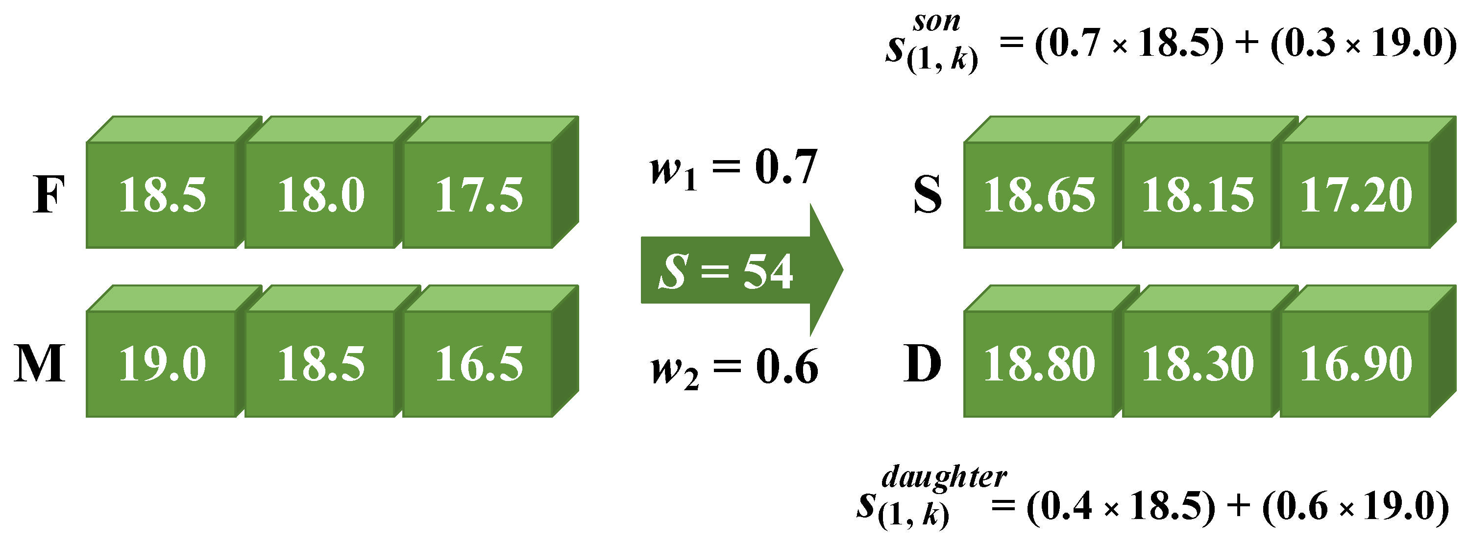
The crossover operation consists of two steps. In Step 1, the crossover is applied to the space allocation list. Using a pair of random numbers $\left(w_k^1,w_k^2\right)\sim U\left[\left(0,1\right)\right], k=1, 2, \dots , P_{size}/2$ for the $k^{th}$ parents, the crossover operator is defined as shown in Equation (31). The crossover operator ensures that the produced offspring are feasible with respect to the space constraint and do not waste storage space.

$$\left.\begin{array}{c}{s}_{\left(m, k\right)}^{son}=w_k^1 ·s_{\left(m, k\right)}^{father}+(1 -w_k^1) · s_{\left(m, k\right)}^{mother}\\ s_{\left(m, k\right)}^{daughter}=(1 -w_k^2) · s_{\left(m, k\right)}^{father}+w_k^2 · {\epsilon }_{\left(m, k\right)}^{mother}\\ m=1, 2, \dots , M; k=1, 2, \dots , P_{size}/2 \end{array}\right\}$$

(31)

The crossover operation is applied to the activity list in Step 2 using a two-point crossover technique. In this method, two individuals are randomly selected from the population, and two crossover points, excluding dummy points, are randomly chosen. The segments between these points are exchanged between the selected individuals to generate new offspring. To maintain the uniqueness of activities in the list, the remaining activities are reinserted in their original order. This process results in two new offspring activity lists.

An illustrative example of the crossover operator applied to the space allocation list and the activity list is shown in Figure 3 and Figure 4, respectively. In these figures, F and M represent the selected parents (father and mother), while S and D represent the two produced offspring (son and daughter).

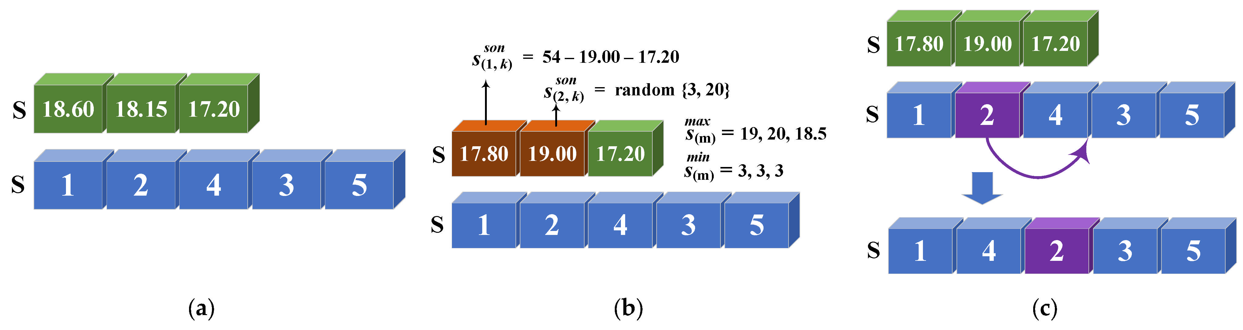
Since the crossover operation is completed, mutation is applied to enhance population diversity. With a probability of $P_m~U\left[\left(0,1\right)\right]$ and if a randomly generated number $p$ satisfies the condition $p<P_m$, the genetic algorithm (GA) performs a mutation operation separately on the two lists of an individual, the space allocation list and the activity list, as shown in Figure 5. Let the current generation be represented by $g$. For the space allocation list, we introduce an interval mutation operator. In this operator, a material $m$ is randomly selected from all available materials, and $s_{\left(m\right)}$ is transformed into a random value within the interval $\left\{s_{\left(m\right)}-{\epsilon }_g ·\left(s_{\left(m\right)}-s_{\left(m\right)}^{min}\right),s_{\left(m\right)}+{\epsilon }_g·\left(s_{\left(m\right)}^{max}+s_{\left(m\right)}\right)\right\}$ where ${\epsilon }_g=1 -g/G_{max}$. If the mutated space allocation list is infeasible or results in inefficient use of space, we randomly adjust $s_{\left(\omega \right)},\omega \in M\setminus \left\{m\right\}$ until the allocation becomes feasible. For the activity list, the mutation operator is applied to each gene. To ensure precedence constraints are met, the feasible positions ($p^{fs}$) for an activity must be placed after all its predecessors and before all its successors. The activity is then randomly inserted into a new feasible position.

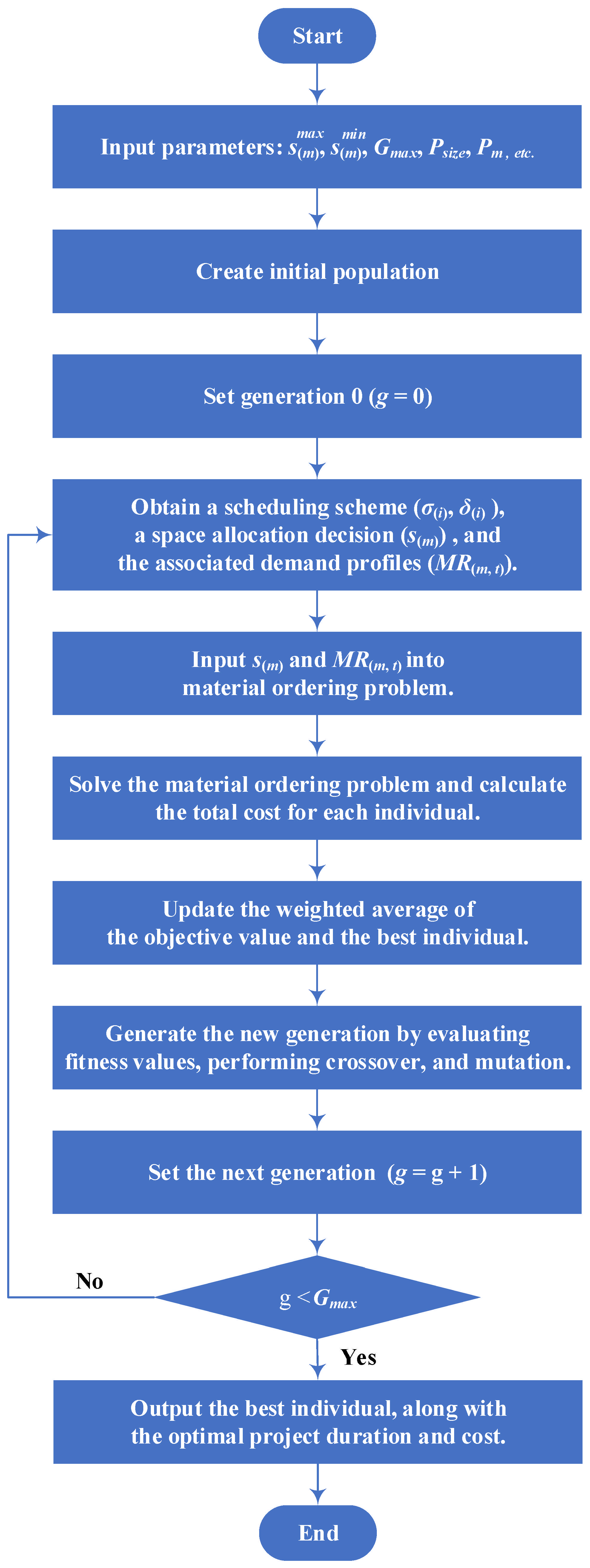
Subsequently, the feasibility of the resulting activity sequences is assessed. After verification, activity delays are adjusted within the project scheduling layer, and a material ordering plan is developed based on the updated activity sequence. The overall structure of the 3LGA, as outlined through the steps described above, is illustrated in Figure 6.

The 3LGA was implemented using Visual Basic for Applications (VBA) within Microsoft Excel (version 2111 build 16.0.14701.20254). This software was selected due to its ability to manage complex data structures, automate iterative calculations, and facilitate the integration of multiple decision-making layers.

The data flow between the three layers—space allocation, project scheduling, and material ordering—was managed through structured VBA coding as follows:

• The space allocation layer processed data related to available storage capacities and allocated materials accordingly, ensuring efficient space utilization.
• The project scheduling layer received inputs from the space allocation layer and adjusted activity timelines to align with storage constraints, ensuring smooth project progression.
• The material ordering layer used the information from both the space allocation and scheduling layers to determine optimal material ordering times, minimizing storage durations while ensuring timely material availability.

The integration of these layers was automated using VBA, ensuring accurate, efficient, and seamless data flow across the system. This approach minimized manual input, reduced processing errors, and enhanced the overall efficiency of the 3LGA implementation.

5. Numerical Experiments

A project case study with 10 activities and three types of materials was generated using RanGen (version 3.2.8) software. The project network is shown in

Table 2. Project case study.

ID	Activity	Predecessor	Duration	Quantity of Required Materials
				M1	M2	M3
1	A	-	1	7	6	2
2	B	-	2	2	2	2
3	C	1, 2	4	6	6	10
4	D	-	2	1	10	1
5	E	-	5	8	8	10
6	F	3	10	8	1	2
7	G	1, 2	10	9	7	7
8	H	3, 4, 5	1	6	10	9
9	I	3, 4, 5	9	4	6	6
10	J	6, 7	7	4	1	10

. It is assumed that ${IC}_{\left(m\right)}$ = 2 for all $m$ = 1, 2, 3, meaning the inventory cost of each type of material is identical. Similarly, the unit ordering cost for each type of material is assumed to be the same; specifically, ${OC}_{\left(m\right)}$ = 50 for all $m$ = 1, 2, 3. The unit indirect cost ($C_I$) is set at 50 per unit period. Additionally, the total storage space for materials at the project site ($S$) is limited to 54 units, with the size of storage space of each material per unit capacity ($v_{\left(m\right)}$) assumed to be one unit per item. For this project, the 3LGA was used, employing a population ($P_{size}$) of 100 individuals per generation and running ($G_{max}$) for 1500 generations, with iterations performed to improve the solution.

The 3LGA experiment, based on the aforementioned case study project, is divided into two scenarios. In the first scenario, a 100% weight is assigned to project cost, focusing exclusively on minimizing costs. In the second scenario, a 100% weight is assigned to project duration, focusing solely on minimizing the project’s duration.

In the genetic algorithm (GA), each generation consists of a population ($P_{size}$) of 100 individuals per generation and running ($G_{max}$) for 1500 generations, with a mutation rate of 0.1. To automate data computation for the case study project, the mathematical model and GA are implemented through Visual Basic for Applications (VBA).

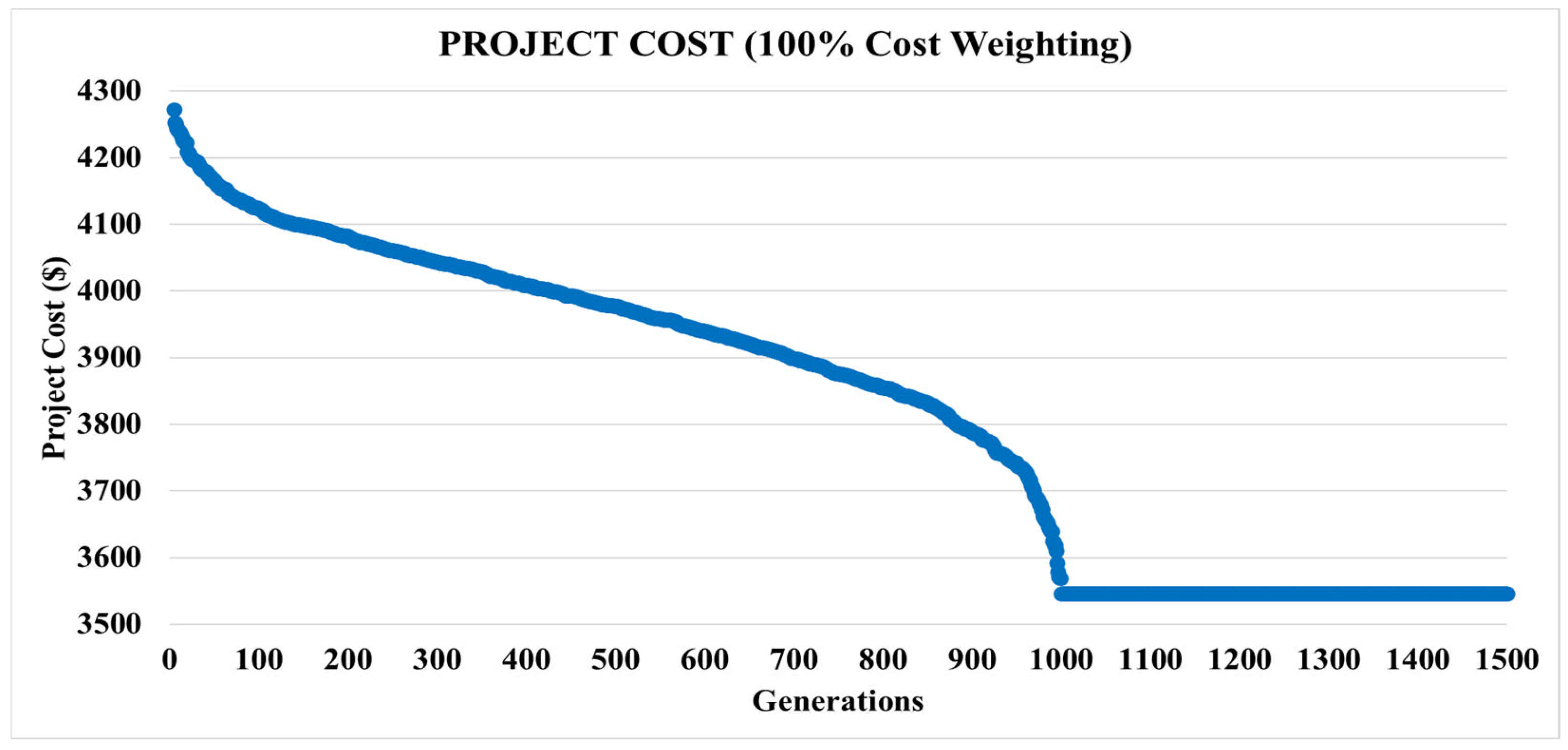
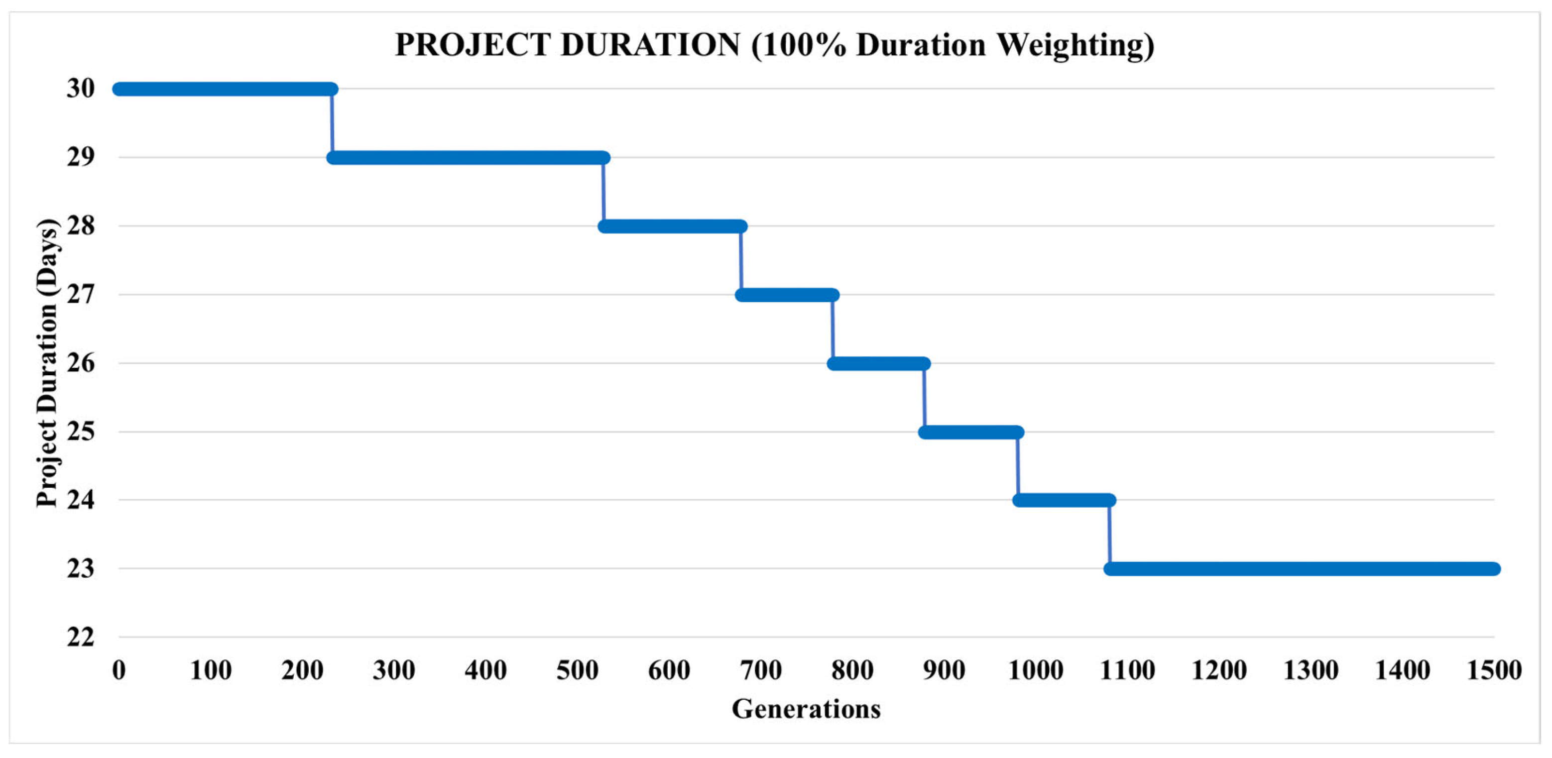
The improvements achieved by the 3LGA in project cost (in the 100% cost weighting scenario) and project duration (in the 100% duration weighting scenario) are illustrated in Figure 7 and Figure 8, respectively.

As shown in Figure 7, in the scenario with a 100% weight on project cost, the 3LGA significantly reduces costs. The best solution from the first generation decreases by 18% by the final generation (generation 1500), from USD 4309 to USD 3546. Similarly, Figure 8 demonstrates that in the scenario with a 100% weight on project duration, the 3LGA reduces the best solution by 23% by the final generation (generation 1500), from 30 days to 23 days.

Additionally, the results of the space allocation plan, ordering plan, project duration, and project cost obtained from the 3LGA experiment using the ordering strategy based on the time period (OSTP) are compared with those derived using the ordering strategy based on the activity (OSA) [3]. These comparisons, presented in

Table 3. Optimal solution (100% cost weighting) comparing between OSA and 3LGA.

Approach	${\mathit{s}}_{\left(\mathit{m}\right)}$	${\mathit{q}}_{\left(\mathit{m},\mathit{t}\right)}$	Period																									PD	PC
			1	2	3	4	5	6	7	8	9	10	11	12	13	14	15	16	17	18	19	20	21	22	23	24	25
OSA [3]	18.00	$q_{\left(1,t\right)}$	17		6				18									14										25	4214
	18.00	$q_{\left(2,t\right)}$	16		6				18									17
	18.00	$q_{\left(3,t\right)}$	14		10				10									15	10
3LGA	18.50	$q_{\left(1,t\right)}$	18.1				9.9	5.7			3.4			11.8		5.3				0.1				0.4	0.2			23	3546
	18.00	$q_{\left(2,t\right)}$	7.5	7.1	9.7	12.3					3.2	3.1		9.4	1.2		3.4	0.1	0.0
	17.50	$q_{\left(3,t\right)}$	6.9		13.7			15.3			3.4	7.9			1.2			8.0		0.0	2.1	0.3	0.0		0.1

(100% cost weighting) and

Table 4. Optimal solution (100% duration weighting) comparing between OSA and 3LGA.

Approach	${\mathit{s}}_{\left(\mathit{m}\right)}$	${\mathit{q}}_{\left(\mathit{m},\mathit{t}\right)}$	Period																									PD	PC
			1	2	3	4	5	6	7	8	9	10	11	12	13	14	15	16	17	18	19	20	21	22	23	24	25
OSA [3]	18.00	$q_{\left(1,t\right)}$	17		6				18								14											24	4170
	18.00	$q_{\left(2,t\right)}$	16		6				18								16		1
	18.00	$q_{\left(3,t\right)}$	14		10				10								15		10
3LGA	17.80	$q_{\left(1,t\right)}$	11.0	7.7	7.9		3.4		10.7	2.0			9.9			1.7					0.2			0.2	0.2			23	3570
	18.00	$q_{\left(2,t\right)}$	8.8	14.1		13.0		0.6	3.5			10.1		5.5	0.3		0.9			0.2
	18.20	$q_{\left(3,t\right)}$	3.5	6.1		11.3		3.2	9.2			14.5		4.8							2.9		2.5		1.0

(100% duration weighting), clearly indicate that the 3LGA is significantly more effective than the OSA in solving the PSMOP-LSS, producing substantially lower project costs and durations.

The 3LGA approach has the potential to generate significant cost savings in construction projects. By optimizing material delivery schedules and minimizing storage durations, the approach reduces costs associated with prolonged storage, material handling, and potential material damage. Although a direct quantitative comparison with traditional methods was beyond the scope of this study, simulation results suggest that the 3LGA method can reduce overall material handling and storage costs by an estimated 15% (reducing from USD 4214 to USD 3546 as shown in Table 3). However, further empirical validation is recommended for a more precise economic assessment in diverse project contexts.

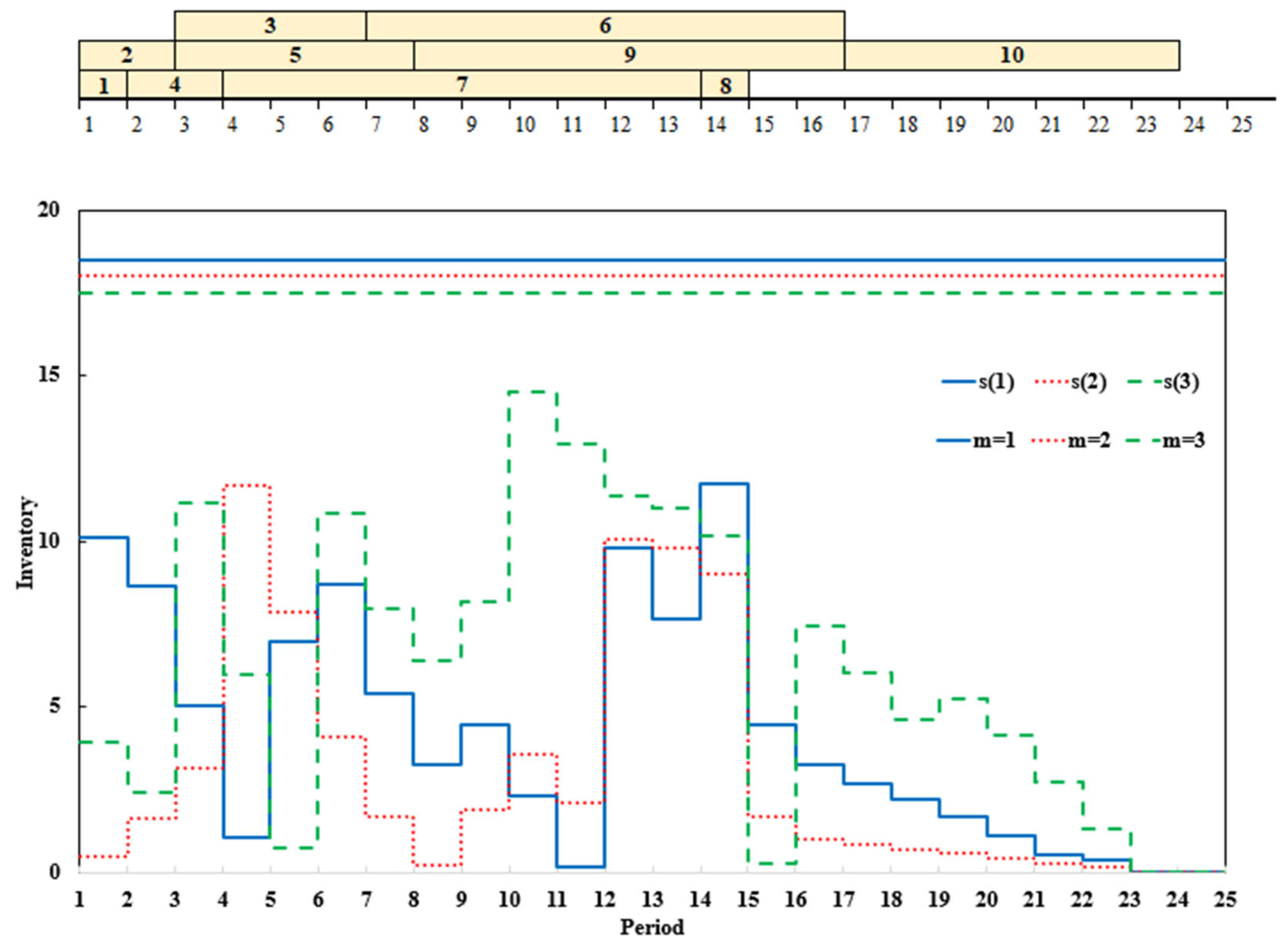
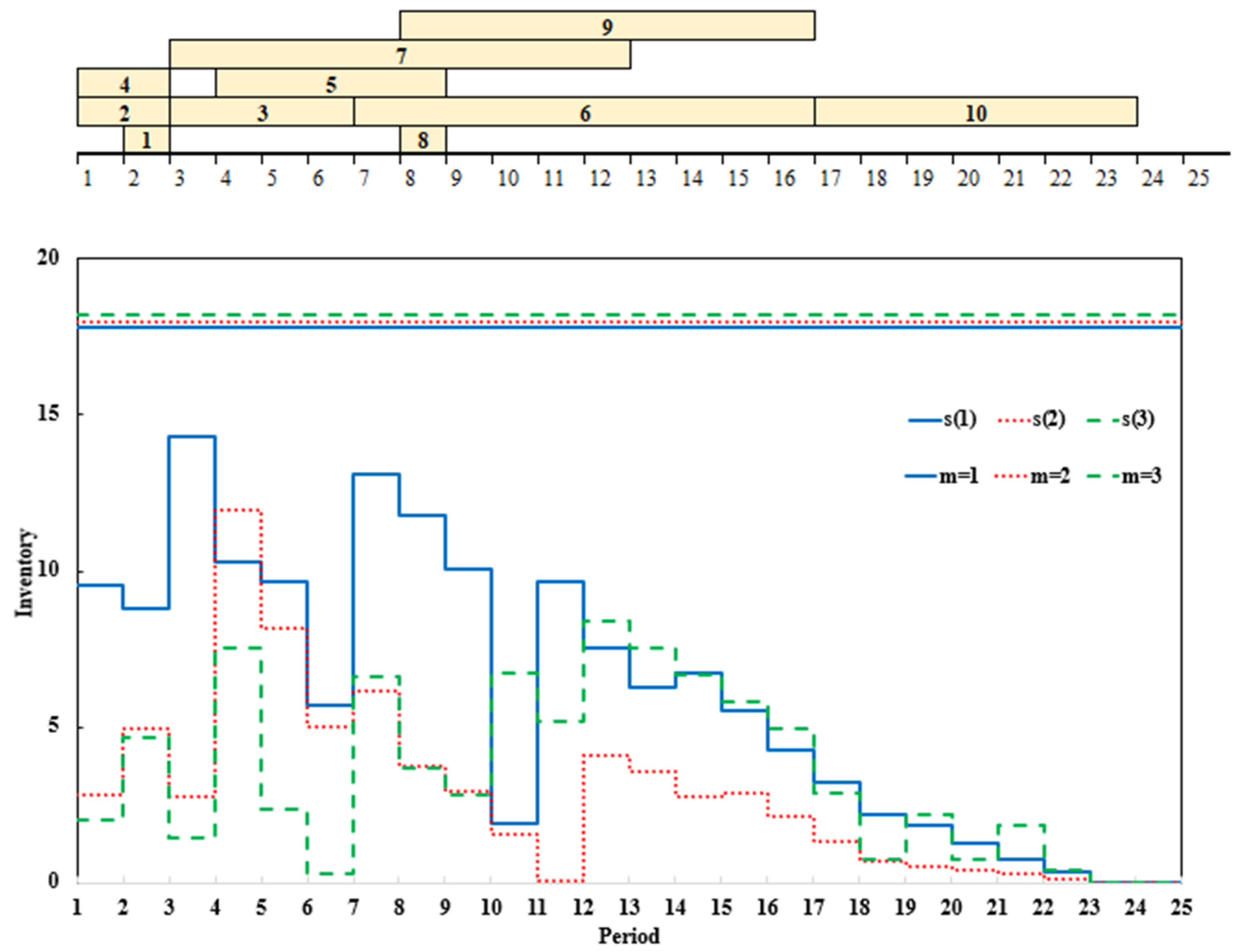
The corresponding Gantt charts for project scheduling and material inventory levels using 3LGA are shown in Figure 9 (100% cost weighting) and Figure 10 (100% duration weighting).

6. The Relationship Between Parameters

In practice, a project has inherent characteristics, including total storage space, ordering cost per order, inventory cost per unit, and indirect cost per unit period, which influence other parameters of the PSMOP-LSS. These factors are critical in making trade-offs between parameters to achieve optimal project outcomes, as outlined in the following subsections.

6.1. Total Storage Space

The relationship between total storage space and project duration is significant, as shown in Figure 11. Greater storage space typically shortens project duration by allowing larger quantities of materials to be ordered and stored, which enables activities to start earlier and run in parallel. However, limited storage space results in fewer materials being stored, delaying activities and extending the project timeline.

When storage capacity is large, fewer orders are needed, as larger quantities can be purchased at once. Conversely, limited space increases the number of orders due to smaller purchase quantities, as illustrated in Figure 12.

A large storage capacity also enables bulk purchasing, reducing the frequency of orders and lowering ordering costs, as shown in Figure 13. In contrast, limited storage space leads to smaller, more frequent orders, which increases ordering costs.

When a construction project has more storage space, it results in a shorter duration, which reduces indirect costs (Figure 14). Conversely, less storage space leads to a longer project duration and higher indirect costs.

With more storage space, bulk purchasing increases inventory, raising inventory costs (Figure 15). Limited storage space results in smaller purchases and lower inventory costs.

Finally, as shown in Figure 16, when storage space increases, both ordering and indirect costs decrease. The reduction in these costs is typically greater than the increase in inventory costs, leading to an overall decrease in project costs.

6.2. Ordering Cost per Order

The relationship between ordering cost per order and project duration, as shown in Figure 17, indicates that higher ordering costs per order tend to shorten project duration. This is because high ordering costs encourage bulk purchasing, which makes shipping more economical and reduces overall ordering costs. Bulk purchasing allows activities to begin earlier, enabling parallel work and faster completion. In contrast, a low ordering cost per order reduces the incentive for bulk purchasing, leading to insufficient materials for simultaneous activities, which delays task initiation and lengthens the project duration.

As illustrated in Figure 18, the relationship between ordering cost per order and the number of orders is such that higher ordering costs result in fewer orders due to bulk purchasing, which makes shipping more cost-effective. On the other hand, lower ordering costs lead to more orders, as materials can be purchased in smaller quantities more frequently.

Figure 19 shows that the relationship between ordering cost per order and total ordering cost is such that higher ordering costs increase the overall cost of purchasing materials. Conversely, lower ordering costs reduce the total cost of purchasing materials.

The relationship between ordering cost per order and inventory cost, as depicted in Figure 20, shows that higher ordering costs typically lead to higher inventory costs. This is because bulk purchasing, which is necessary for cost-effective shipping, results in a larger surplus of materials that must be stored. In contrast, lower ordering costs tend to reduce inventory costs, as there is less emphasis on shipping efficiency, allowing for smaller orders.

Figure 21 demonstrates the relationship between ordering cost per order and indirect costs. Higher ordering costs generally reduce indirect costs because bulk purchasing enables the early start of multiple activities, allowing for parallel work and faster project completion. Conversely, with lower ordering costs, there is less incentive to purchase in bulk, which may delay the start of tasks due to limited material availability, leading to longer project durations.

Finally, Figure 22 illustrates the relationship between ordering cost per order and overall project cost, which includes ordering, inventory, and indirect costs. When ordering costs increase, the combined ordering and inventory costs tend to rise faster than the reduction in indirect costs, leading to higher project costs. Conversely, when ordering costs decrease, the reduction in ordering and inventory costs typically outweighs the increase in indirect costs, resulting in a lower overall project cost.

6.3. Inventory Cost per Unit

The relationship between inventory cost per unit and project duration, as shown in Figure 23, indicates that when the inventory cost per unit increases, materials must be ordered in smaller quantities to avoid excessive surplus, which would raise inventory costs. Ordering materials in smaller quantities limits material availability, reducing the likelihood of starting activities earlier and preventing multiple activities from running in parallel, which leads to a longer project duration. In contrast, when the inventory cost per unit decreases, larger quantities of materials can be ordered without concern for excessive inventory costs, ensuring that enough materials are available for multiple activities to proceed simultaneously, thus accelerating project completion.

The relationship between inventory cost per unit and the number of orders, as shown in Figure 24, reveals that when the inventory cost per unit increases, materials must be ordered in smaller quantities to avoid excessive surplus and storage. This results in multiple orders to meet the needs of various activities throughout the project. Conversely, when the inventory cost per unit decreases, there is less concern about surplus materials, allowing for larger orders and reducing the number of orders.

The relationship between inventory cost per unit and ordering cost, as shown in Figure 25, demonstrates that when the inventory cost per unit increases, materials must be ordered in smaller quantities to reduce daily storage volumes, leading to more frequent orders. Conversely, when the inventory cost per unit decreases, larger orders can be made, thereby reducing the number of orders.

The relationship between inventory cost per unit and overall inventory cost, as shown in Figure 26, indicates that when the inventory cost per unit increases, overall storage costs tend to rise. Conversely, when the inventory cost per unit decreases, overall storage costs tend to decrease as well.

The relationship between inventory cost per unit and indirect costs, as shown in Figure 27, shows that when the inventory cost per unit increases, materials must be ordered in smaller quantities to avoid excessive surplus, which raises inventory costs. This limited material availability reduces the chances of starting activities earlier and running multiple activities in parallel, leading to a longer project duration and higher indirect costs. In contrast, when the inventory cost per unit decreases, larger orders can be made without excessive concern for inventory costs, ensuring enough materials for parallel activities and speeding up project completion, thus reducing indirect costs.

Finally, the relationship between inventory cost per unit and project cost, which includes ordering costs, inventory costs, and indirect costs, as shown in Figure 28, demonstrates that when the inventory cost per unit increases, ordering costs, inventory costs, and indirect costs tend to rise, resulting in a higher overall project cost. Conversely, when the inventory cost per unit decreases, all three costs tend to decrease, leading to a lower overall project cost.

6.4. Indirect Cost per Period

The relationship between indirect cost per unit period and project duration, as shown in Figure 29, suggests that when the indirect cost per unit period increases, the project duration tends to decrease. This is because the project manager accelerates construction operations to reduce overall indirect costs. In contrast, when the indirect cost per unit period decreases, the project duration increases, as the project manager does not need to expedite construction operations.

The relationship between indirect cost per unit period and the number of orders, as shown in Figure 30, shows that when the indirect cost per unit period increases, the project manager must accelerate construction operations. This leads to ordering larger quantities of materials at once to ensure sufficient materials are available for simultaneous activities, thereby reducing the number of orders. Conversely, when the indirect cost per unit period decreases, the project manager does not need to rush construction operations, allowing for smaller orders to be placed over time, which results in an increased number of orders.

The relationship between indirect cost per unit period and ordering cost, as shown in Figure 31, indicates that when the indirect cost per unit period increases, the project manager must expedite construction operations. This results in larger orders at once and fewer orders overall, which in turn reduces ordering costs. Conversely, when the indirect cost per unit period decreases, the project manager does not need to speed up construction operations, allowing for smaller, more frequent orders, ultimately reducing ordering costs.

The relationship between indirect cost per unit period and inventory cost, as shown in Figure 32, illustrates that when the indirect cost per unit period increases, the project manager must accelerate construction operations, leading to larger orders of materials. This increases the amount of inventory stored each day and raises inventory costs. In contrast, when the indirect cost per unit period decreases, the project manager does not need to rush construction operations, allowing for smaller, more frequent orders. This reduces the inventory that needs to be stored daily and lowers inventory costs.

The relationship between indirect cost per unit period and indirect costs, as shown in Figure 33, demonstrates that when the indirect cost per unit period increases, overall indirect costs tend to rise. Conversely, when the indirect cost per unit period decreases, overall indirect costs tend to decrease.

Finally, the relationship between indirect cost per unit period and project cost, which includes ordering costs, inventory costs, and indirect costs, as shown in Figure 34, reveals that when the indirect cost per unit period increases, the combined inventory and indirect costs tend to rise at a rate greater than the decrease in ordering costs, resulting in an overall increase in project costs. Conversely, when the indirect cost per unit period decreases, the combined inventory and indirect costs tend to decrease at a rate greater than the increase in ordering costs, leading to a reduction in project costs.

7. Conclusions

This paper proposes an integrated project scheduling and material ordering problem with limited storage space (PSMOP-LSS) aimed at minimizing project costs and duration. Unlike previous studies, this research introduces a concurrent planning approach for storage space allocation, activity timetabling, and material ordering under storage space constraints. To optimize material ordering, a space-saving ordering strategy (OSTP) is also employed. The space-saving ordering strategy (OSTP) is an approach designed to optimize material ordering schedules by minimizing on-site storage requirements. The strategy focuses on timing material deliveries as close as possible to the scheduled usage date, thereby reducing the duration and volume of materials stored on-site. This is particularly beneficial in space-constrained construction environments. For example, if a construction project requires large quantities of steel beams at a specific phase, the OSTP ensures that these materials are ordered and delivered just before their scheduled use. This approach avoids early deliveries that would otherwise require prolonged on-site storage, thus reducing storage congestion and minimizing the risk of material deterioration or loss. Within the 3LGA framework, the OSTP integrates with the material ordering layer to optimize delivery schedules, enhancing both efficiency and space utilization.

A genetic algorithm (GA) was developed to solve the PSMOP-LSS, with the model divided into three layers of solution analysis: the space allocation layer (SA), the project scheduling layer (PS), and the material ordering layer (MO). This layered approach effectively addresses the NP-hard nature (a classification of computational problems for which no known algorithm can solve all instances efficiently in polynomial time) of the problem, enabling simultaneous optimization of space allocation, project scheduling, and material ordering.

The triple-layer genetic algorithm (3LGA) was developed based on the ordering strategy based on the time period (OSTP), which is more effective than the ordering strategy based on the activity (OSA) in the context of project scheduling and material ordering problems with limited storage space (PSMOP-LSSs) for several reasons. These two strategies differ significantly in their approach to managing material deliveries and scheduling tasks, especially when dealing with storage constraints, procurement schedules, and material handling costs. Below is a detailed explanation of why the OSTP offers advantages over the OSA:

• Optimizing material ordering to match storage constraints
  • OSA limitation: The ordering strategy based on the activity (OSA) orders materials based on the specific requirements of each task or activity in the project. While this approach works well in scenarios where storage space is unlimited, it does not account for the capacity limitations of storage space. This may lead to situations where materials are delivered too early or too late, resulting in idle inventory, overcrowded storage areas, and material rehandling—factors that increase project costs and delays.
  • OSTP advantage: In contrast, the ordering strategy based on the time period (OSTP) schedules material deliveries in a way that aligns with time periods in the project schedule. By considering the time frame for each construction phase, it ensures that materials are delivered exactly when needed, optimizing storage space utilization. The OSTP prevents overstocking and understocking, minimizing the space required for storage.
• Improved coordination with procurement schedules
  • OSA limitation: The OSA assumes that materials are ordered based on the specific activities to be carried out, but it does not consider the variability in procurement lead times or external delivery schedules. In many real-world construction projects, especially those with tight schedules or complex logistics, procurement delays or early deliveries can create a mismatch between material availability and task requirements, leading to inefficiencies.
  • OSTP advantage: The OSTP better accounts for procurement lead times and delivery schedules by considering material availability over time. Materials can be ordered in a more structured way according to the overall project timeline, making it easier to synchronize procurement with construction activities. This approach minimizes stockpiling and reduces the risks of material shortages or excess stock.
• Reduction in storage space utilization and material handling costs
  • OSA limitation: In the OSA, materials are delivered as needed for each individual task or activity, often leading to inefficient use of available storage space. Without considering the broader project timeline, multiple deliveries of the same material may occur over time, increasing space utilization, storage costs, and the need for additional handling.
  • OSTP advantage: The OSTP optimizes material ordering by grouping deliveries according to the project’s time periods. This reduces the frequency of deliveries and associated handling costs. As a result, construction projects can manage their storage space more effectively, ensuring that materials are delivered in larger, consolidated shipments that align with project milestones. This leads to reduced material handling, lower storage costs, and better space management.
• Handling project complexity and task dependencies
  • OSA limitation: The OSA works well when task dependencies and material requirements are straightforward, but it does not efficiently manage the complex interdependencies between tasks and materials in large-scale projects. When multiple tasks depend on materials at different times, the OSA may struggle to coordinate deliveries and storage for all tasks, leading to congestion in the storage area and potential delays.
  • OSTP advantage: The OSTP can better manage these complexities by grouping materials based on the time periods in which they are needed. This approach allows for more strategic management of task dependencies, as materials can be delivered in a coordinated way across multiple tasks. This reduces the likelihood of bottlenecks and optimizes the use of available storage space, making it easier to manage both material flow and storage across the entire construction project.
• Better adaptation to dynamic construction environments
  • OSA limitation: The OSA tends to be more rigid in its material ordering approach because it focuses solely on task-specific needs rather than the overall project timeline. This lack of flexibility can be problematic when dealing with unexpected changes in the project, such as delays or scheduling shifts.
  • OSTP advantage: The OSTP, by contrast, is more adaptable to changes in the project environment because it is based on time periods rather than individual activity requirements. This allows greater flexibility in adjusting material delivery schedules in response to changes in project timelines, procurement lead times, or unforeseen delays. It is better suited to handle the dynamic nature of construction projects, which is essential for maintaining efficient operations and staying on schedule.

Projects typically exhibit inherent characteristics, such as the number of activities, resource requirements, precedence relationships, available storage space capacity, and cost parameters. As such, project managers must carefully consider these factors and balance trade-offs between total cost and project duration when scheduling activities and making material ordering decisions. The managerial insights from this study are summarized as follows:

If materials are expensive or difficult to store, resulting in high inventory costs per unit, project managers should order materials frequently in small batches. However, they must also account for the potential impact of extended project durations, which can increase indirect costs.

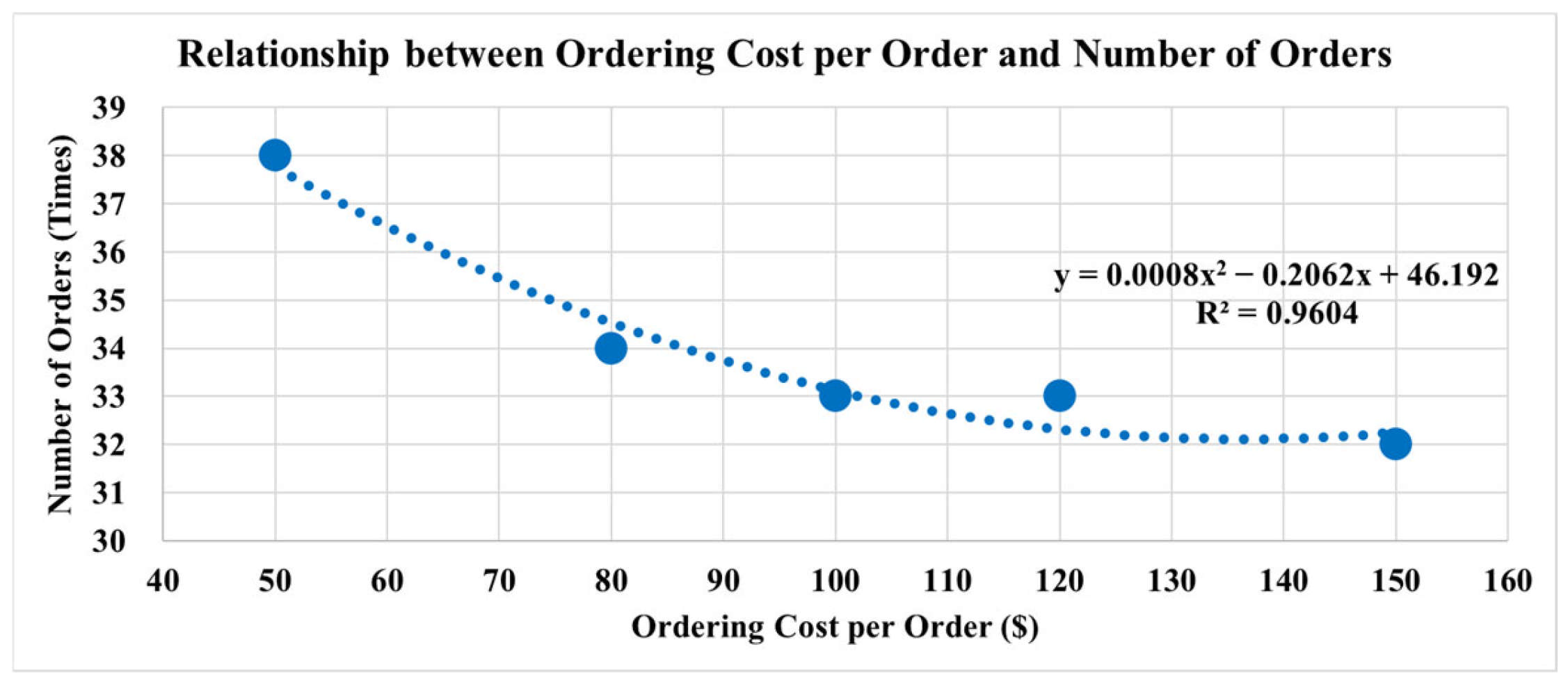
Conversely, if material transportation is difficult and expensive, indicating high unit ordering costs, materials should be ordered in larger quantities to reduce order frequency.

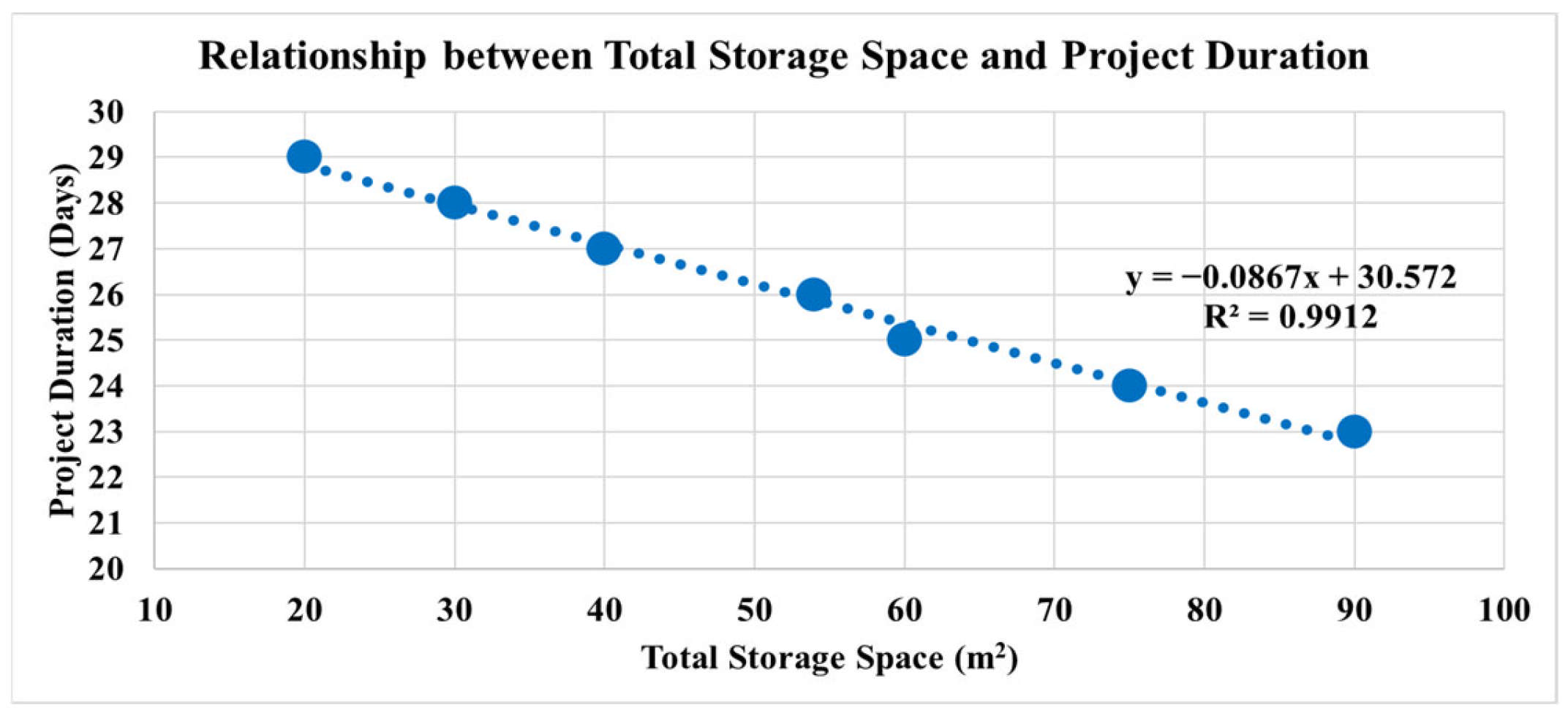
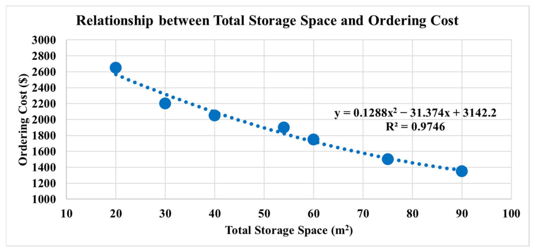
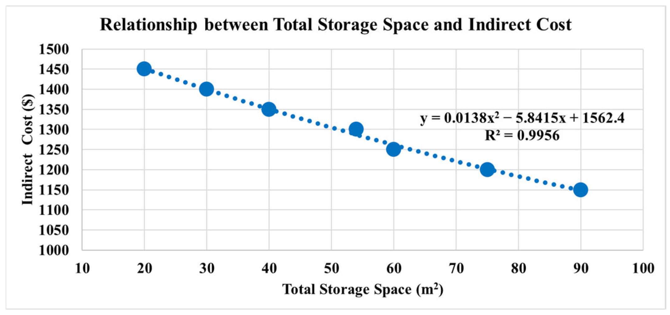
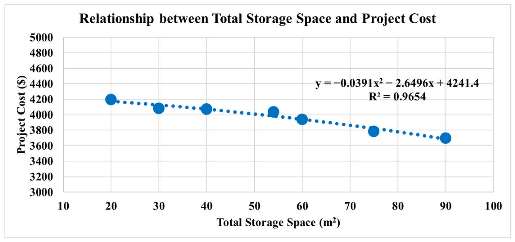
Increasing storage space can lower project costs and shorten project durations. Therefore, project managers should evaluate whether expanding storage capacity is worthwhile by weighing its cost against the potential savings in project costs and duration.

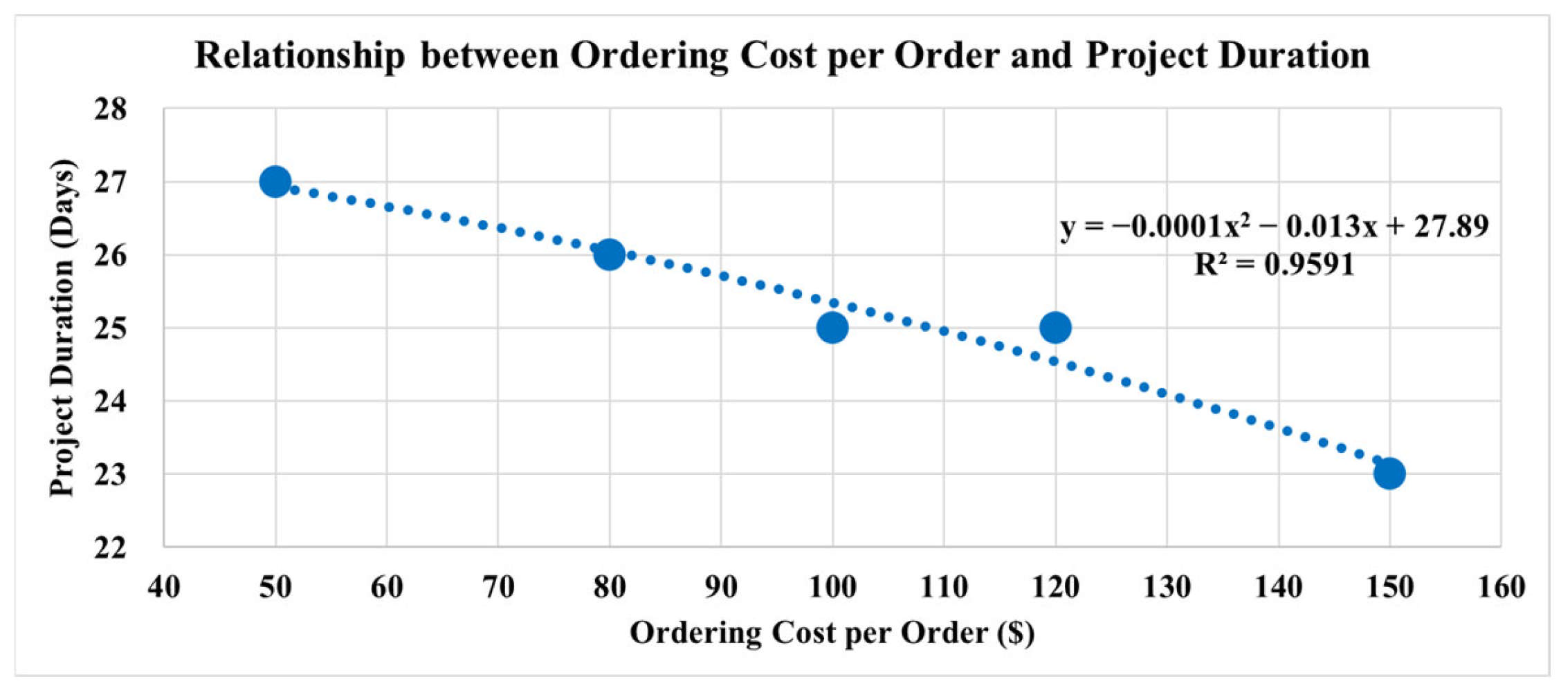
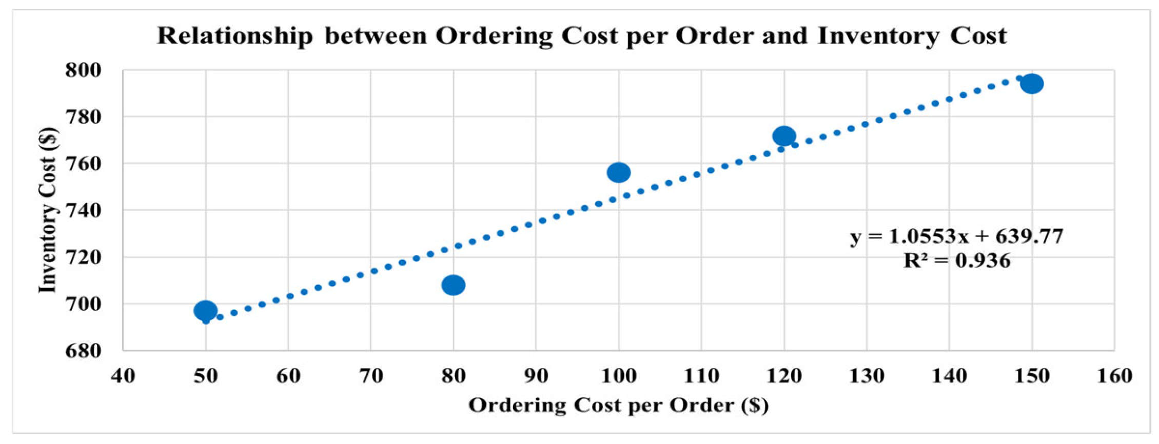
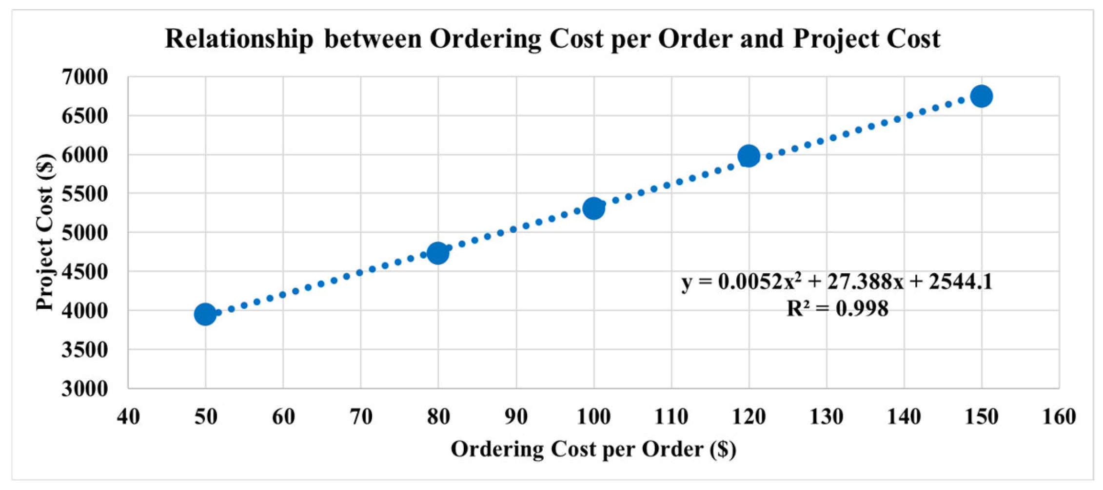
In cases where the ordering cost per order increases, it can lead to higher project costs but shorter project durations. Project managers must decide whether to prioritize cost minimization or faster completion. For example, if ordering costs are high and large quantities of materials are ordered at once, the project may finish sooner. However, the reduction in indirect costs might not offset the increased ordering and inventory costs, potentially resulting in higher overall costs.

Real-world projects often involve budget and due date constraints. The proposed model offers a set of genetic algorithm solutions to help project managers navigate these limitations. For instance, when working within a limited budget, managers can select a solution that provides the shortest project duration within the budget.

By addressing limited storage space, this study advances the integrated project scheduling and material ordering problem with a novel extension, providing project managers with more comprehensive decision-making support. However, material demand is often uncertain and may vary during project execution. Exploring the integrated project scheduling and material ordering problem under stochastic demand conditions is a promising area for future research.

To implement the 3LGA (triple-layer genetic algorithm) for the project scheduling and material ordering problem with limited storage space (PSMOP-LSS) in real-world projects, several practical challenges must be addressed. These challenges primarily revolve around software integration, data availability, and other technical constraints that could impact the algorithm’s performance in a dynamic, real-world environment.

1.

Software integration

One of the primary challenges in implementing the 3LGA for the PSMOP-LSS in real projects is integrating the algorithm with existing project management software. Many construction projects rely on proprietary software platforms for scheduling, inventory management, and space planning. Adapting the 3LGA to seamlessly integrate with these systems can be complex and time-consuming. This requires the following:

• Custom software development: the 3LGA may need to be customized to ensure compatibility with project management software, including integrating data input/output and synchronizing project parameters (e.g., scheduling, material ordering) between the algorithm and the software tools.
• API development: creating an API (application programming interface) for communication between the 3LGA and existing systems may be necessary, ensuring real-time data on project schedules, resources, and material availability are shared efficiently.
• User interface considerations: the algorithm should be user-friendly, enabling project managers and planners to interact with it effectively without requiring advanced technical knowledge. An intuitive interface is critical for users to input and modify project data.

2.

Data availability

The accuracy and effectiveness of the 3LGA depend on the availability of accurate, real-time data. This is essential for generating optimal solutions for project scheduling and material ordering. The challenges related to data availability include the following:

• Real-time data collection: The 3LGA requires access to up-to-date data on project timelines, resource availability, procurement lead times, and material costs. Establishing an automated process for real-time data collection and updates is crucial to avoid delays and inaccuracies in the optimization process.
• Data accuracy and consistency: Inconsistent or inaccurate data can significantly impact the algorithm’s performance. Ensuring data accuracy involves collecting real-time data and validating them against established standards and historical data. This may require integrating data validation tools and quality control processes.
• Collaboration among stakeholders: Effective implementation requires collaboration between project managers, suppliers, contractors, and other stakeholders to share and maintain accurate data. Communication protocols may need to be developed to facilitate data exchange between all parties involved in the project.
• Data security and privacy: Since the 3LGA relies heavily on data sharing, ensuring data security is a significant concern. Measures such as encryption methods and secure cloud-based platforms for storing and processing data must be put in place to protect sensitive project data.

3.

Scalability and adaptability

Another challenge is ensuring that the 3LGA can scale to handle the complexity of large projects. Large-scale construction projects involve numerous tasks, materials, and coordination challenges, and the algorithm must be adaptable to handle varying project sizes and types without compromising performance. This may involve the following:

• Scalable architecture: The algorithm must efficiently handle both small and large projects. It should be designed to scale up or down based on the size and complexity of the project.
• Handling uncertainty and dynamic changes: Construction projects often face delays, scope changes, and other uncertainties. The 3LGA must adapt to such changes in real time, adjusting material ordering and scheduling plans as needed.

4.

Training and implementation

To effectively implement the 3LGA in real-world projects, the project team must be trained to use the algorithm. This involves the following:

• Training project managers and planners: Those responsible for managing the project must understand how the 3LGA works, how to input data, and how to interpret the results. A comprehensive training program should be developed to ensure effective usage of the system.
• Change management: Adopting a new system like the 3LGA may require changes in traditional project scheduling and material ordering processes. Proper change management practices should be implemented to ensure a smooth transition and minimize resistance from stakeholders.

5.

Cost and resource considerations

Implementing the 3LGA can incur significant upfront costs, including software development, hardware infrastructure, and training. These costs must be balanced against the potential benefits, such as improved project efficiency and reduced material costs. Project teams will need to assess the return on investment (ROI) for implementing the 3LGA in each specific project context.

While the implementation of the 3LGA for the PSMOP-LSS offers significant benefits in terms of optimization, addressing practical challenges related to software integration, data availability, scalability, and resource allocation is critical for ensuring the algorithm’s effectiveness in real-world projects. By focusing on seamless software integration, ensuring data accuracy, and maintaining adaptability to changing project conditions, the 3LGA approach can be successfully implemented to improve project scheduling and material ordering in complex construction environments.

The 3LGA approach provides practical benefits for construction projects, particularly in urban or space-constrained environments. By optimizing material delivery schedules and minimizing on-site storage durations, the 3LGA approach reduces space congestion and enhances the efficiency of material handling compared to traditional methods. This advantage is particularly significant in projects with limited storage space, where effective logistical planning is critical.

However, it is important to acknowledge the current limitations of the method. Validation was conducted using a simplified case study involving 10 activities and three types of materials to demonstrate the feasibility and effectiveness of the approach. Extending the 3LGA method to larger and more complex projects, characterized by higher numbers of activities, materials, and constraints, remains challenging due to computational complexity. Future research will focus on refining the algorithm to improve its scalability and applicability to more complex construction scenarios.

While the 3LGA method demonstrates significant potential for optimizing material delivery and storage management, several challenges may arise during real-world implementation:

• Data interoperability: Real-world construction projects often involve multiple data sources and formats. Integrating data across the three layers of 3LGA—space allocation, project scheduling, and material ordering—can be complex. Ensuring data compatibility and seamless communication between systems is essential for effective implementation. Adopting standardized data formats and integration protocols can help mitigate this challenge.
• Computational complexity: As project size and complexity increase, so does the computational demand of the 3LGA. Managing larger datasets with multiple constraints could lead to longer processing times and increased resource requirements. Future research may focus on optimizing the algorithm’s efficiency to enhance its scalability for complex projects.
• Requirement for skilled personnel: Implementing and maintaining the 3LGA approach, particularly when utilizing VBA coding within Excel, requires personnel with specialized skills in algorithm development, data management, and computational analysis. Training and capacity-building initiatives can help overcome this barrier and support effective deployment.

Addressing these challenges is essential to ensure the broader applicability of the 3LGA method in complex and dynamic construction environments. Future work will focus on developing strategies to overcome these limitations, including algorithm refinement and integration with more advanced software platforms. While the current study demonstrates the effectiveness of the 3LGA approach in optimizing cost and duration, it is important to acknowledge that the experiments were conducted based on single-run simulations. As such, statistical measures, including confidence intervals and standard deviations across multiple runs with different random seeds, were not calculated. We recognize that performing multiple runs would provide deeper insights into the stability and robustness of the proposed method. Therefore, future research will focus on conducting extensive simulations with varying random seeds and reporting statistical metrics to enhance the reliability and generalizability of the results. This will further validate the consistency and practical applicability of the 3LGA approach.

While the current study focuses on validating the integrated 3LGA approach—which optimizes space allocation, project scheduling, and material ordering—an ablation study was not conducted. Such a study, where one or more layers are removed to analyze their individual impact on optimization performance, could provide deeper insights into the significance and contribution of each layer. Future research will focus on conducting an ablation analysis by systematically removing one layer (e.g., optimizing only scheduling and ordering or ordering and storage) and comparing the results with the fully integrated approach. This will help to assess the individual and collective contributions of each layer, further validating the necessity and effectiveness of the integrated 3LGA model.

The 3LGA approach addresses an NP-hard optimization problem involving space allocation, project scheduling, and material ordering. While the current study successfully validates the feasibility and effectiveness of the approach, it does not include a detailed computational complexity analysis. As such, the scaling behavior of the algorithm’s runtime with increasing problem size (e.g., number of activities, material types, and storage constraints) remains an area for further investigation. Understanding how computational time and resource requirements grow with problem complexity is critical for ensuring the scalability of the 3LGA approach. Therefore, future research will focus on conducting a formal complexity analysis, including empirical evaluations of runtime performance and theoretical assessments using computational complexity notations (e.g., big-O analysis). Additionally, strategies for enhancing computational efficiency—such as optimizing genetic algorithm parameters, implementing parallel processing, or developing heuristic simplifications—will be explored to support the application of 3LGA in large-scale construction projects.

In this study, the hyperparameters for the 3LGA approach—including population size, mutation rate, and crossover rate—were primarily selected based on prior research and standard practices in genetic algorithm design. Initial values were further refined through preliminary trial-and-error experiments to balance optimization quality and computational efficiency. For instance, the mutation rate was set to 0.05, and the population size was set to 100, based on observed solution stability and convergence behavior during preliminary tests. However, a systematic hyperparameter optimization process (such as grid search, random search, or meta-heuristic tuning) was not conducted. This is acknowledged as a limitation that may affect the reproducibility and optimal performance of the algorithm. Future research will focus on employing systematic tuning approaches to identify the most effective hyperparameter settings and assess their influence on both solution quality and computational performance. This will enhance the robustness and reliability of the 3LGA approach for broader applications.

The 3LGA approach adopts a weighted-sum method to optimize the dual objectives of cost and duration. A formal sensitivity analysis to systematically evaluate the impact of varying weight parameters on solution outcomes was not conducted. This is acknowledged as a limitation of the current study. Future research will focus on performing a detailed sensitivity analysis to assess the robustness of the solutions against different weight configurations. Such analysis will provide deeper insights into how the weighting scheme affects optimization outcomes and will enhance the generalizability of the 3LGA approach for diverse project scenarios.