Article

Comparison of Methodologies for the Behavior Factor Estimation in Seismic Design of Buildings: Case Study of Geo-Sourced Masonry Construction

by
Noura Zarzour
1,2,
Maria Paola Santisi d’Avila
1,*,
Andrea Penna
3,4,
Luca Lenti
5 and
Michel Oggero
2
1
Polytech Lab, UPR 7498, Université Côte d’Azur, 930 Route des Colles, 06903 Nice, France
2
FILIATER, 06100 Nice, France
3
Department of Civil Engineering and Architecture (DICAr), University of Pavia, 27100 Pavia, Italy
4
European Centre for Training and Research in Earthquake Engineering, EUCENTRE Foundation, 27100 Pavia, Italy
5
CEREMA, Repsody, Sophia Antipolis, 06903 Valbonne, France
*
Author to whom correspondence should be addressed.
Buildings 2025, 15(7), 1036; https://doi.org/10.3390/buildings15071036
Submission received: 27 February 2025 / Revised: 18 March 2025 / Accepted: 21 March 2025 / Published: 24 March 2025
(This article belongs to the Special Issue Recent Scientific Developments on the Mechanics of Masonry Structures)

Abstract

:
The behavior factor, which represents the force reduction that a structure would experience if its response was completely elastic compared with the seismic forces used for design, is defined in seismic design codes for common construction techniques and materials. A specific assessment is needed when novel construction materials are adopted. The lack of accurate structural performance estimations limits the use of green construction materials because building codes only allow the use of minimum values for the behavior factor. This research aims to verify the reliability of the proposed capacity-demand-based (CDB) method for the estimation of the force reduction factor and behavior factor, by comparison with other procedures such as demand-based, capacity-based and formula-based approaches. The main characteristic of the proposed approach is that the ductility-FRF curve is obtained numerically for the building natural period, instead of imposing an analytical FRF-ductility-period relationship. The advantage of the CDB-method is its efficiency from a computational point of view without restrictions concerning the construction material and structural typology. The results are compared in the case where dynamic analyses are performed for a three-dimensional (3D) building model (considered as a reference) and for an equivalent single-degree-of-freedom system which reduces the computation time. The CDB-method yields safe results compared with the N2 method, and it is consistent with a capacity-based approach applied to the 3D building model.

1. Introduction

The interest in soil-based construction materials is increasing, aiming to mitigate carbon emissions associated with conventional types of structures and materials adopted for buildings. The growing demand for green materials requires the estimation of parameters used in building design according to seismic codes. Structural design is normally performed considering that materials are used within their elastic range for the involved loads; however, seismic codes introduce a parameter named the behavior factor to allow the use of linear analysis and force-based seismic design methods also in the case of relatively rare events inducing nonlinear structural responses with damage propagation and consequent energy dissipation. Force-based seismic design approaches represent the seismic demand as a distribution of lateral forces whose total sum (base shear force) mainly depends on masses and an acceleration response spectrum, varying with the return period of the seismic action at the site, divided by the behavior factor. The latter allows for the reduction in design seismic forces, considering the favorable effect of the plastic deformations associated with the ductility of the structure.
International seismic codes provide behavior factor estimations for common construction materials and structural typologies, but the growing use of geo-sourced materials requires specific research (Bocciarelli [1], Hummel and Seim [2], Aloisio et al. [3], Gubana and Mazelli [4]). The uncertainty of the performance of low-carbon construction materials, and in particular masonry wall systems, in regions susceptible to seismic activity may restrict their utilization, and a reliable estimation of the behavior factor can boost construction using geo-sourced and sustainable materials.
This research aims to compare the results obtained using different approaches for the estimation of the behavior factor, highlighting the impact of the assumptions, to better understand their variability and their potential application in professional practice for novel construction materials.
According to Uang [5], the behavior factor q is mainly related to the force reduction factor (FRF), reflecting the structural capacity to dissipate hysteretic energy. The FRF is defined as the ratio between the maximum force (related to a maximum displacement) attained in linear elastic and elasto-plastic analysis. In the case of buildings, the base shear and top displacement are assumed, respectively, as representative force and displacement parameters.
The maximum strength in an elasto-plastic analysis is defined more easily by adopting a bilinear idealization (Tomaževič [6], Tomaževič et al. [7]) of the first-loading curve. Since in the bilinear idealization, the yield base shear force is obtained numerically and it is not associated with the yielding of a structural element, Uang [5] estimates the behavior factor as the FRF corrected by a factor named the overstrength ratio (Blume [8]). This is estimated as the ratio between the yield force in the idealized elasto-perfectly-plastic curve and the yield force attained when the first structural element reaches its conventional lateral strength capacity (Morandi [9], Magenes [10]). The overstrength ratio can also be defined as the ratio between the yield base shear force in the bilinear idealization and the force demand prescribed by the seismic design code (Uang [5], Fajfar [11]).
The FRF is linked through a causal relationship to the structure displacement ductility (Chopra [12], Priestley et al. [13]), conceptually defined as the maximum to yield displacement ratio. The determination of the maximum base shear force in linear elastic conditions, for the estimation of the FRF (ratio between the maximum base shear force in linear elastic and elasto-plastic analysis), can be carried out by imposing a conceptual hypothesis (yielding an analytical FRF-ductility-period relationship). Accordingly, the estimation of the FRF is performed through nonlinear quasi-static (pushover) analysis combined with the iso-displacement or iso-energy criteria (Veletsos and Newmark [14], Newmark and Hall [15]), or more developed assumptions (Vidiç et al. [16], Fajfar [17], Guerrini et al. [18]). On the other hand, the maximum base shear force in linear elastic conditions can be estimated for a base shear force related to a maximum top displacement that is obtained for a given seismic load. This seismic load can be fixed as the seismic demand (demand-based approach) or related to the structural collapse (capacity-based approach). Consequently, in the demand-based method, the maximum top displacement is related to the seismic demand; instead, in the capacity-based method it is set according to the definition of structural collapse. In this case, the FRF is predicted by coupling pushover and dynamic analysis (Mwafy and Elnashai [19], Mohsenian et al. [20]). Some research has been performed to compare demand-based and capacity-based approaches to determine the FRF (Mwafy and Elnashai [19], Mohsenian et al. [20], Hussain et al. [21]).
In the framework of pushover analysis, the FRF is influenced by the selected load distribution along the building height, in each load direction. In the case of dynamic analysis, the estimation of the FRF is repeated for a set of ground acceleration time histories, on a statistical basis. In particular, in the capacity-based method, the seismic load amplitude associated with the structural collapse must be determined. In this context, the incremental dynamic analysis (IDA) proposed by Vamvatsikos and Cornell [22] is a numerical tool allowing the assessment of the peak ground acceleration (PGA), for a given waveform, related to a fixed ultimate top displacement of the structural system, in an inelastic analysis. Moreover, the FRF estimation can be performed for a three-dimensional (3D) building model or an equivalent single-degree-of-freedom (SDOF) system (Saiidi and Sozen [23], Chopra and Goel [24], Fajfar [25]).
Zarzour et al. [26] propose a methodology to estimate the FRF and then the behavior factor, integrating both seismic demand and building capacity. For this reason, this methodology can be considered as a capacity-demand-based approach for FRF estimation. A correlation between the FRF q 0 and the ductility demand μ d is obtained for a set of synthetic seismic signals compatible with the seismic demand represented by the elastic response spectrum of the European seismic design code [27]. It is assumed that the structural materials are used within their elastic range for the involved loads. Consequently, the elastic limit is related to the seismic demand and therefore to a fixed FRF q 0 . The attained ductility μ d , for the seismic demand (and fixed FRF q 0 ), is deduced by performing a dynamic analysis for an equivalent SDOF system having an equivalent natural period and the building damping ratio. On the other hand, the ductility capacity μ c is obtained by a pushover analysis using a 3D numerical model of the building. The FRF related to the building ductility capacity μ c is obtained from its ductility-FRF curve.
This capacity-demand-based method is applied for the seismic design of a rubble stone masonry building (Zarzour et al. [26]) and a pilot compressed earth block masonry building (Zarzour et al. [28]). The stability verification of the building structure at the near collapse limit state is performed using a force-based approach (equivalent lateral force analysis in which the seismic base shear is defined using the estimation of the behavior factor) and a displacement-based approach (capacity to demand displacement ratio), both performed as specified in the European building code. Zarzour et al. [26,28] verify the building stability also in terms of the capacity-to-demand load ratio (base shear force ratio). In fact, since the estimation of the ultimate displacement is significantly dependent on the accuracy of the numerical procedure, the stability verification in terms of displacement could be affected. Moreover, this is inspired by the Italian code [29] in which a limit of four is imposed for the target load ratio q 0 d , obtained as the elastic target load at the near collapse limit state normalized with respect to the yield base shear force of the building. According to Zarzour et al. [26], it is verified that the target load ratio q 0 d does not exceed the force reduction factor q 0 of the building. Comparing the capacity-to-demand ratios in terms of displacement and load obtained by Zarzour et al. [26,28], the stability verification in terms of force is more restrictive in some instances.
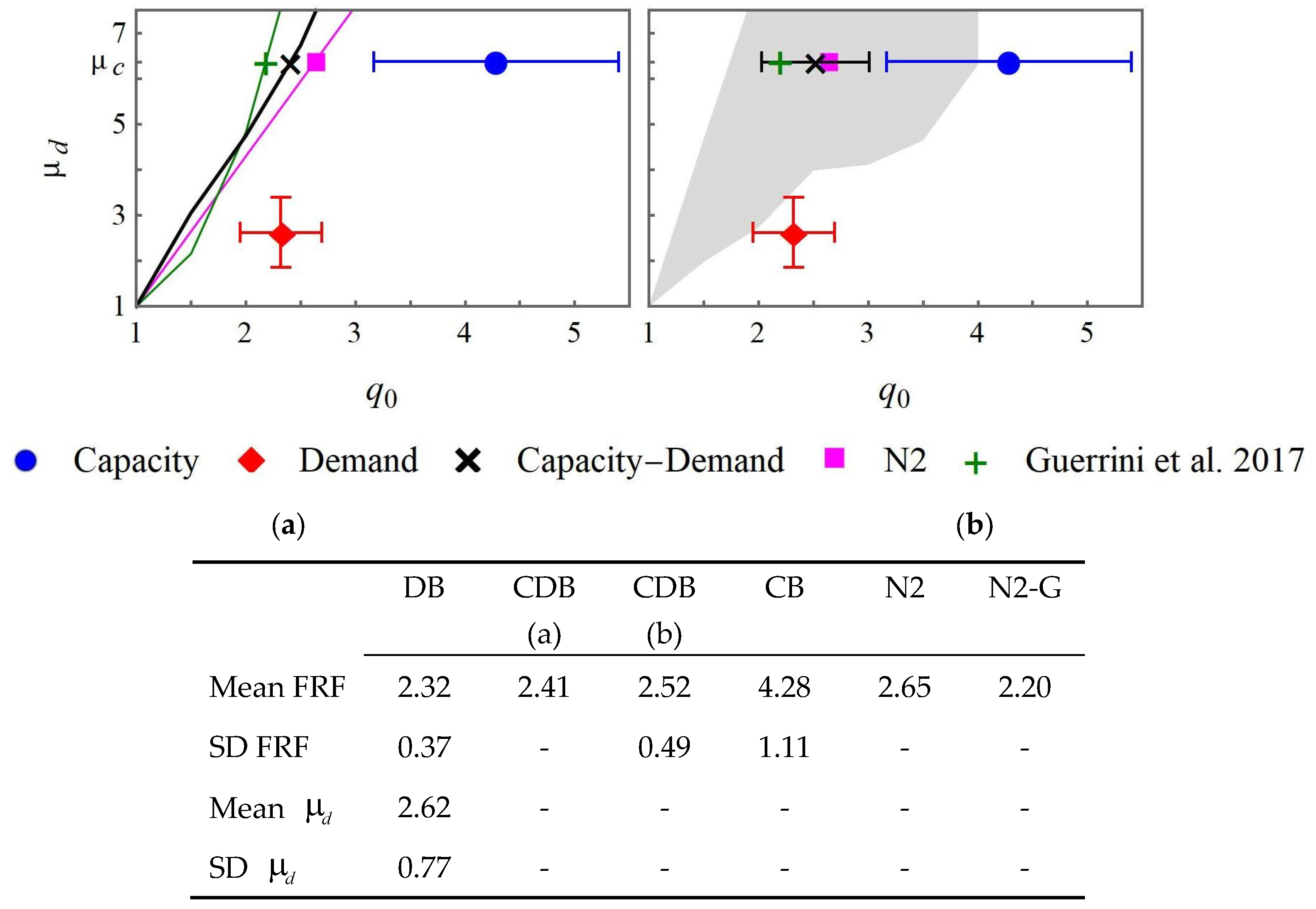
The aim of this research is the comparison of the capacity-demand-based method with the demand-based, capacity-based and formula-based approaches, to prove its reliability and efficiency for professional practice. In particular, the analyzed methodologies are applied in this research to building structures composed of load-bearing masonry walls. The impact on the obtained FRF of adopting a 3D building model or an equivalent SDOF system is investigated. In addition, the obtained results are compared with the FRF estimated using the N2 method (Fajfar [17]), as presented in the Eurocode 8 [27], and also using the correction proposed by Guerrini et al. [18] which is specifically calibrated for masonry buildings, characterized by a short fundamental period.
The FRF estimation is carried out for a three-floor rubble stone masonry building. The masonry building is modeled using the equivalent frame method and the discretization approach proposed by Lagomarsino et al. [30], in which the masonry bearing walls are decomposed in deformable wall elements (piers and spandrels) connected by rigid nodes. The equivalent frame model, developed as a strategy for the seismic analysis of both new and existing unreinforced masonry buildings, is recommended in the European seismic code [27].
In the first part of this study, piers and spandrels are modeled using a beam-element (Galasco et al. [31]) with elasto-perfectly-plastic behavior. This modeling technique is implemented in the 3Muri software by S.T.A. DATA (release 13.9.0.1), which can be used easily in professional practice. Then, masonry wall elements are modeled using the same equivalent frame discretization but with the macro-element developed by Penna et al. [32] (implemented in the research version of the software), which better reproduces the hysteretic behavior in nonlinear dynamic analysis.
In this paper, the methodologies for estimating the FRF and behavior factor are presented in Section 2. The building model is discussed in Section 3. The results obtained from the different approaches are discussed in Section 4. The conclusions are developed in Section 5.

2. Methodologies for the Behavior Factor Estimation

According to Uang [5], the behavior factor q = q 0   O S R is mainly related to the FRF q 0 , corrected by multiplying it by the overstrength ratio O S R (Morandi [9], Magenes [10]). The FRF is the ductility-dependent component of the behavior factor, reflecting the structural capacity to dissipate hysteretic energy.
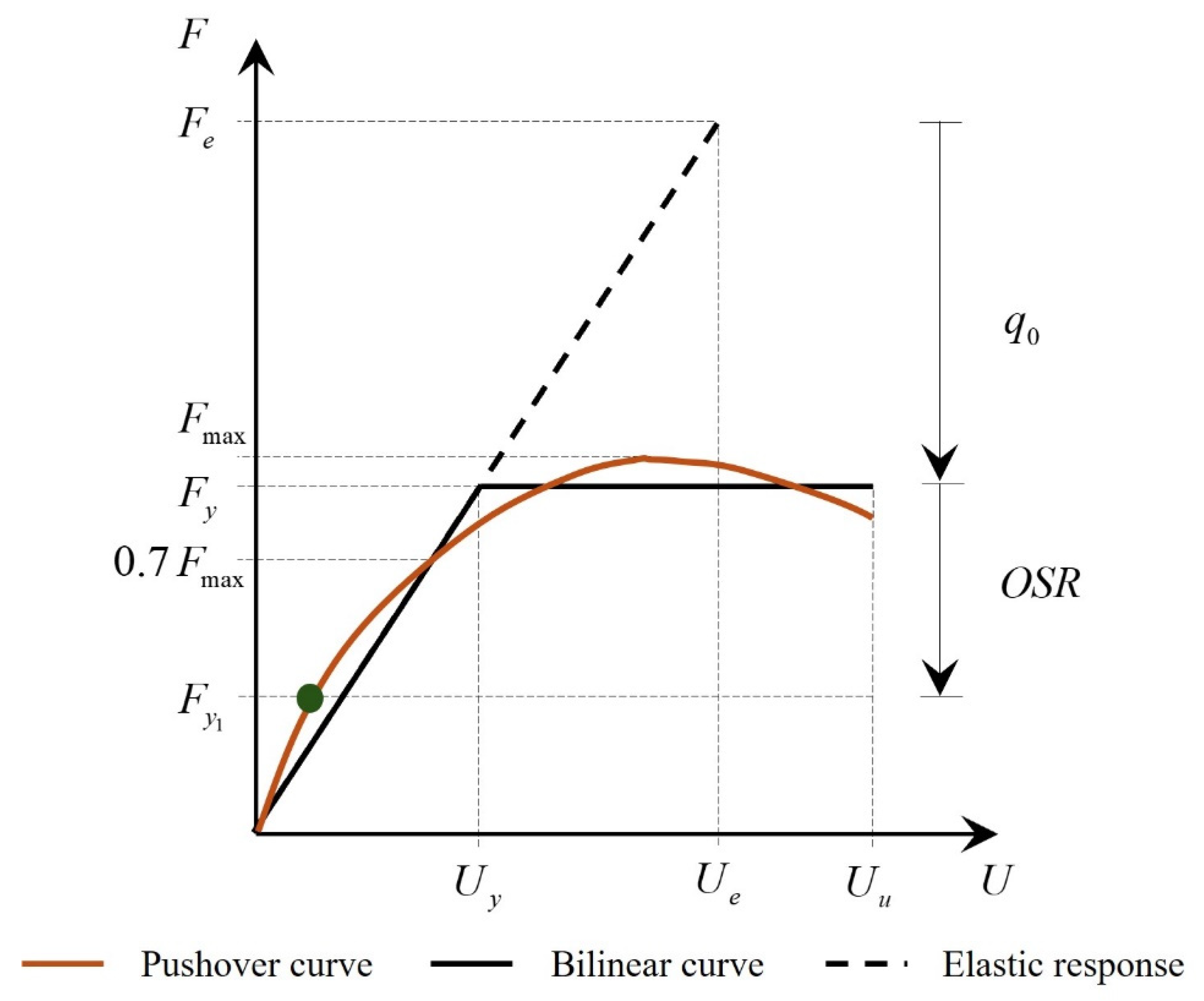
The result of a pushover analysis is the so-called pushover curve of the building, representing the relation between the base shear force and the top floor lateral displacement. The pushover curve is meant to approximate the average envelope of the cyclic response obtained in a dynamic analysis (Galasco et al. [31]). The bilinear idealization of the pushover curve (Figure 1) allows the definition of a yield base shear F y , corresponding with the plateau. This also allows the estimation of the FRF
q 0 = F e / F y
as the ratio between the base shear force F e in linear elastic conditions and F y . As the yield base shear force F y is obtained numerically in the bilinear idealization and it is not associated with the yielding of a structural element, the overstrength ratio O S R   =   F y / F y 1 is defined as the ratio between the yield base shear force F y and the base shear force F y 1 attained when the first structural element reaches its lateral strength. The first significant yield, which is used to determine the overstrength ratio, is indicated in Figure 1 with a thick point. The structure displacement ductility μ is conceptually defined as the maximum to yield top displacement ratio (Chopra [12], Priestley et al. [13]). In a bilinear idealization of the pushover curve, U y is related to the yield base shear force F y . The ductility demand μ d = U max / U y , where the maximum top displacement U max is related to the seismic demand, is distinguished from the ductility capacity μ c = U u / U y , where the ultimate displacement U u is set according to the definition of structural collapse. The same definitions can be extended to the first-loading curve in a dynamic analysis.
In this research, the bilinear idealization of the pushover curve is obtained by imposing an initial stiffness secant to the point where F = 0.7   F max (Tomaževič [6]) on the curve, where F max is the maximum base shear attained during the pushover analysis (Figure 1), and then the yield force F y is obtained according to an equivalence of energy (equal areas below the pushover and bilinear curve up to the ultimate displacement).
The FRF (Equation (1)) depends on the elastic base shear force F e estimation, which is directly influenced by the seismic load amplitude. According to Mohsenian et al. [20], if the seismic load is specified by the building code, the FRF is estimated according to a demand-based (DB) method. Otherwise, if the seismic load amplitude is set corresponding with the attainment of the building ultimate capacity, the FRF is estimated according to a capacity-based (CB) method.
In the following analysis, capital letters are adopted for forces and displacements of a pushover curve F , U , or first-loading curve in a dynamic analysis, obtained using a 3D building model. Additionally, lowercase letters indicate the same parameters in a capacity curve f , u , for an equivalent SDOF system, obtained by scaling the pushover curve and using the modal participation factor Γ as a scaling constant. The latter is estimated by normalizing the mode shape with respect to its value at the top level.
Pushover and dynamic analyses applied to a 3D building model have the advantage of accounting for the geometry of the building and the constitutive behavior of wall elements. On the contrary, the use of an equivalent SDOF system reduces the computational cost of the numerical procedure adopted for the FRF estimation.

2.1. Demand-Based Force Reduction Factor

In a DB-approach, the seismic load amplitude corresponds to the seismic demand specified in the adopted building code (Mohsenian et al. [20]). The DB-FRF is estimated following the next steps:
-
The seismic demand is represented as ground motion time histories compatible with the elastic response spectrum, according to some compatibility criteria generally defined in the building code.
-
A nonlinear pushover analysis is carried out using the 3D model of the building and the yield base shear force F y is obtained from the bilinear idealization of the pushover curve (Figure 1). The pushover curve is meant to approximate the average envelope of the cyclic response obtained in a dynamic analysis (Galasco et al. [31]). Consequently, a nonlinear dynamic analysis could be performed, but the bilinear idealization of the first-loading curve would provide a similar estimation of the yield base shear force F y .
-
A dynamic analysis is performed in a linear elastic regime to estimate the elastic base shear force F e for each seismic signal. The definition of the DB-FRF (Equation (1)) is independent of the modeling strategy adopted for the structural system. The dynamic analysis can be carried out using an equivalent SDOF system or the 3D building model.
-
The DB-FRF is obtained as the ratio q 0 = F e / F y (Equation (1)).
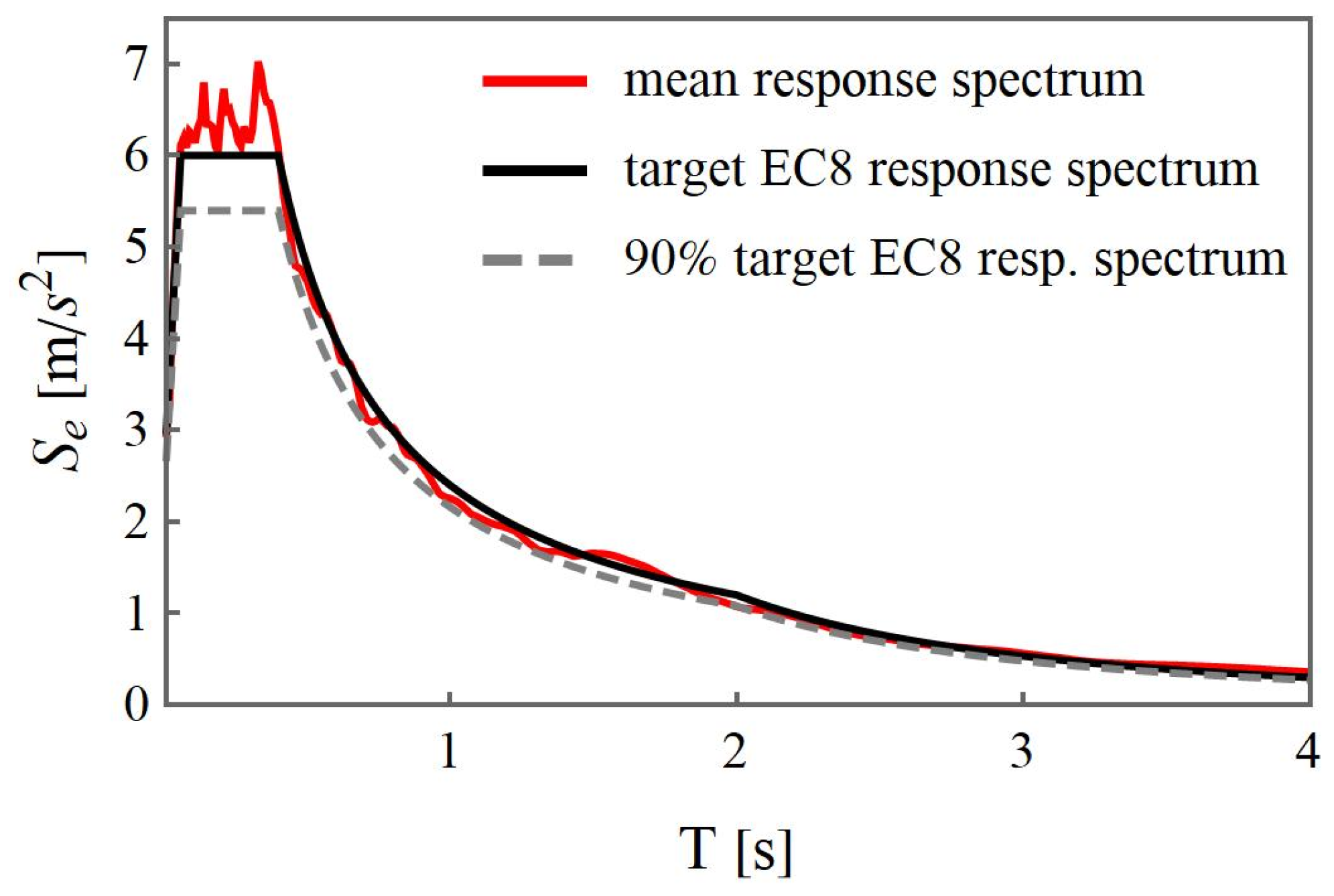
In this research, the generation of synthetic spectrum-compatible seismic signals is performed according to Cacciola et al. [33], verifying the compatibility criteria with the seismic demand, represented by an elastic response spectrum defined by the European building code [27]. Interested readers can refer to Zarzour et al. [26] for more details. Considering that the compatibility is attained for a set of seismic signals, on an average basis, the FRF is then estimated statistically.

2.2. Capacity-Based Force Reduction Factor

In a CB-approach, the seismic load amplitude corresponds to the attainment of the building ultimate capacity (Mohsenian et al. [20]). The CB-FRF is estimated following the next steps:
-
The building ultimate capacity is defined. It can correspond to a fixed reduction in strength (total base shear force) occurring after reaching the peak strength, or a maximum drift attained in a structural element.
-
A nonlinear pushover (or dynamic) analysis is carried out using the 3D model of the building and the pushover (or hysteresis) curve is truncated at the ultimate top displacement U u corresponding with the building ultimate capacity. From the bilinear idealization of the pushover (or first-loading) curve, the yield base shear force F y is obtained (Figure 1).
-
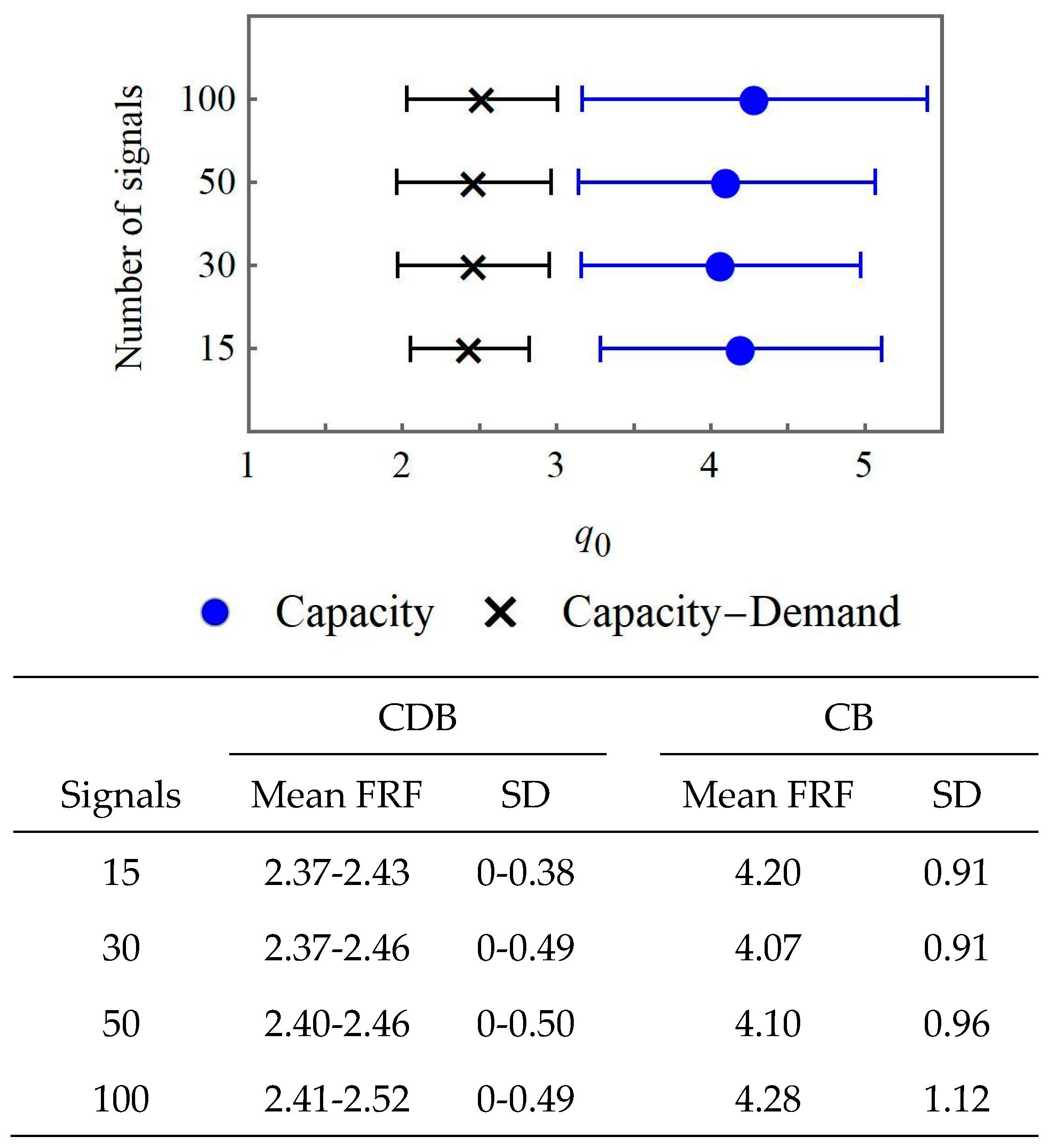
Then, ground motion signals that lead to the building ultimate displacement must be obtained. The scaling of each ground motion signal represents the complexity of this approach. In this research, the spectrum-compatible synthetic ground motion signals (Cacciola et al. [33], Zarzour et al. [26]) are scaled iteratively and the ultimate displacement of the structure for each signal is estimated using nonlinear IDA. The latter is implemented using the hunt-and-fill tracing algorithm (Vamvatsikos and Cornell [22]) to determine the PGA corresponding to the attainment of structure failure during each ground motion time history. The scaling factor is higher than one for building design.
-
A dynamic analysis is performed in a linear elastic regime to estimate the elastic base shear force F e for each scaled seismic signal. The definition of the CB-FRF (Equation (1)) is independent of the modeling strategy adopted for the structural system. The dynamic analysis can be carried out using an equivalent SDOF system or the 3D building model.
-
The CB-FRF is obtained as the ratio q 0 = F e / F y (Equation (1)).
The average CB-FRF is then estimated for the set of scaled seismic signals.

2.3. N2-Based Force Reduction Factor

According to the N2 method proposed by Fajfar [17], which is integrated into the Eurocode 8 [27,34], the displacement demand u d for an equivalent SDOF system having an equivalent natural period T 0 is estimated as
u d = u e d T 0 T C u d = u e d T 0 < T C and f y / m 0 S e T 0 u d = u e d q 0 d 1 + q 0 d 1 T C T 0 u e T 0 < T C and f y / m 0 < S e T 0
where
q 0 d = m 0   S e T 0 / f y
is a load ratio obtained as the elastic target load normalized with respect to the yield base shear force f y in elasto-plastic conditions. S e T 0 is the acceleration provided by the elastic response spectrum for the natural period T 0 and m 0 is the mass of the equivalent SDOF system. The elastic displacement in Equation (2) is calculated as u e d = S e T 0 T 0 / 2 π 2 . Fajfar [17] distinguishes short and medium to long periods of the system through the limit T C which is the corner period between the constant acceleration and constant velocity part of the response spectrum.
After comparing the results obtained by a nonlinear dynamic analysis and the N2 method (Fajfar [17]) in terms of ductility demand, Guerrini et al. [18] consider that the N2 method can underestimate the ductility demand in the case of masonry structures, characterized by a short fundamental period. They propose to estimate the displacement demand u d as
u d = u e d T 0 T C u d = u e d T 0 < T C and f y / m 0 S e T 0 u d = u e d q 0 d q 0 d 1 c ( T 0 / T ¯ + a ) ( T 0 / T C ) b + q 0 d u e T 0 < T C and f y / m 0 < S e T 0
where the parameters a , b , c and T ¯ can be calibrated applying an orthogonal regression between the results of Equation (4) and those of nonlinear dynamic analysis for a set of oscillators. Guerrini et al. [18] propose a set of parameters calibrated specifically for three typologies of masonry structures having different damage mechanisms and hysteretic dissipation (mainly flexure-dominated, intermediate and shear-dominated). In the following computations, the parameters a = 0 , b = 2.3 , c = 2.1 and T ¯ = 0.022   s are adopted assuming a mainly shear-dominated dissipation.
In this research, the N2-based approaches are applied following the next steps:
-
The formulation 2 or 4 is adopted to estimate the peak ground acceleration (at the soil surface) P G A y and P G A u , by imposing that the displacement demand u d is equal to the yield and ultimate displacement u y and u u , respectively. The PGA is involved in the definition of the acceleration response spectrum S e T 0 in Equation (3), obtained as the product of the expected PGA S a g at the soil surface and a term representing the structure amplification. S a g is the product of the peak acceleration at rock outcropping a g amplified by the soil factor, which depends on the ground type.
-
According to Milosevic et al. [35], the CB-FRF is estimated as the PGA ratio (Costa et al. [36]) in ultimate and yielding conditions q 0 = P G A u / P G A y .
First, this procedure allows for understanding if the PGA amplitudes obtained using the IDA tool are consistent. Then, the value obtained by this procedure serves as a comparator to verify the reliability of the FRF obtained using dynamic analysis, according to the DB-, CB- and CDB-approaches.

2.4. Capacity-Demand-Based Force Reduction Factor

Zarzour et al. [26] propose a methodology to estimate the FRF, integrating both seismic demand and building capacity, that can be considered as a capacity-demand-based approach for the FRF estimation. This method is based on the assumption that the structural materials are used within their elastic range for the involved loads. This means that the yield displacement of the equivalent SDOF system is imposed equal to
u y * = S a ( T 0 , q 0 ) T 0 / 2 π 2
so that it is related to the seismic demand S a ( T 0 , q 0 ) and therefore to a fixed FRF q 0 .
The CDB-FRF is estimated following the next steps (Zarzour et al. [26]):
-
The seismic demand is represented as ground motion time histories compatible with the elastic response spectrum, according to some compatibility criteria generally defined in the building code.
-
A nonlinear dynamic analysis is performed for the equivalent SDOF system having a natural period T 0 and damping ratio ζ , shaken by the set of synthetic ground motion signals, using as first-loading curve a modified capacity curve having yield displacement u y * (Equation (5)) and maintaining the stiffness associated with T 0 . The attained ductility μ d = u max / u y is deduced.
-
The analysis is repeated over a range of FRFs q 0 to obtain a correlation between the FRF q 0 and the ductility demand μ d . When the FRF q 0 is modified, the elastic limit changes and, accordingly, the yield base shear force f y for a given equivalent natural period T 0 of the system. Consequently, the attained maximum displacement and the ductility demand change.
-
The ductility-FRF curve is deduced, dependent on the natural period T 0 of the equivalent SDOF system and the building damping ratio ζ . A ductility–FRF curve is obtained for each spectrum-compatible seismic signal.
-
On the other hand, a pushover analysis is performed using the 3D model of the building structure. After having defined the building ultimate condition and consequently the ultimate displacement, the displacement ductility capacity μ c = U u / U y of the building is obtained.
-
Then, the CDB-FRF related to the building ductility capacity μ c is obtained from the average ductility-FRF curve.
Two conditions must be checked for the application of the proposed method, which is based on the assumption that the yield displacement of the equivalent SDOF system corresponds with the seismic demand (Equation (5)). This means that the structure is considered to have elastic behavior until the displacement related to the seismic demand. First, this assumption is verified during the numerical process by controlling that the yield displacement of the equivalent SDOF system u y * , assumed in the dynamic analysis (Equation (5)) during the procedure to obtain the μ d , q 0 curve, for each value of q 0 must be
u y * = S a ( T 0 , q 0 ) ( T 0 / 2 π ) 2 u y
where u y = U y / Γ is the yield displacement derived from the capacity curve (Figure 1).
Additionally, if the seismic demand in elastic conditions is lower than the yield force f y , the response of the equivalent SDOF system is elastic and the ductility is not triggered. For this reason, the second condition to be verified is that the seismic demand in elastic conditions must be higher than the yield force. This can be written as
q 0 d = m 0 S e T 0 / f y 1
where q 0 d is the target load ratio defined in Equation (3), m 0 is the mass of the equivalent SDOF system and S e T 0 is the elastic response spectrum. It is important to verify this condition 7 because otherwise the FRF results are overestimated, especially in the case of high ductility capacity. In the case where q 0 d < 1 , to avoid the overestimation of the FRF, a correction is proposed as follows: the PGA is increased (consequently, the seismic demand S e T 0 in elastic condition is increased) to attain q 0 d = 1 .

3. Three-Dimensional Building Model

The DB-, CB- and CDB-approaches discussed in 
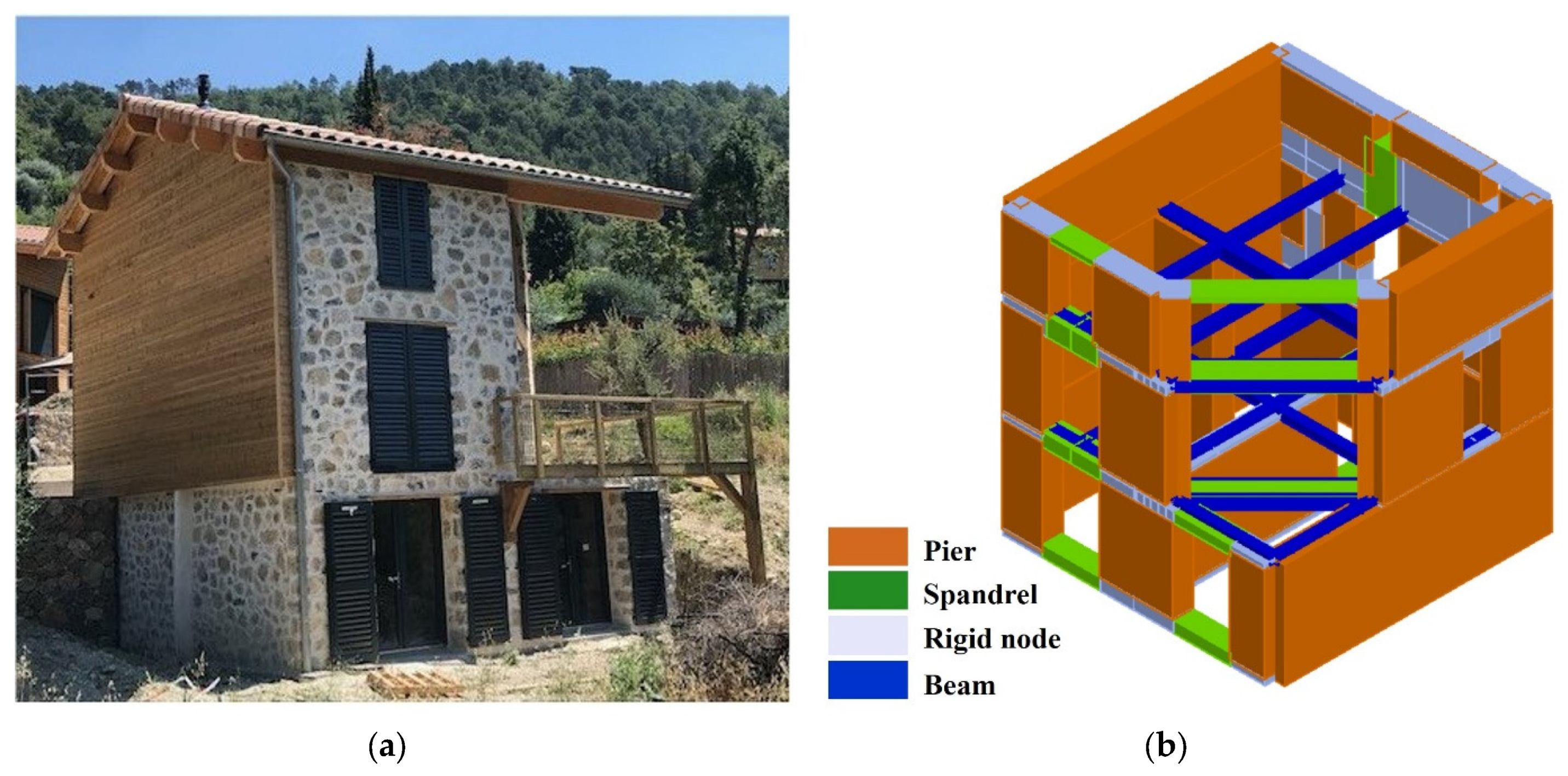
Section 2, for the FRF and behavior factor estimation of a building, are independent of the adopted construction material and bearing structure. A three-story rubble masonry building (Figure 2a) is selected as a case study because of the growing interest in low-carbon construction materials, whose mechanical and ductility parameters must be accurately estimated before being used in structural design, for insurability reasons. Moreover, the small floor area of the selected building reduces the computational effort, allowing the comparison of the analyzed methodologies.
The bearing masonry walls are constructed using local natural stone and earth mortar. The mechanical parameters of the rubble stone masonry, determined through experimental tests on masonry specimens, are summarized in Table 1. The roof and floors are made with glued laminated timber beams, joists and planks. The strength class of the timber is GL24h (characteristic flexural strength equal to 24 MPa). Tie rods connect the walls on each floor to prevent out-of-plane failures and ensure a global box-like behavior under seismic loading. The building is constructed in a moderate seismic hazard zone (zone 4 in the French seismic hazard zonation map) having a design ground acceleration of a g = 1.6   m / s 2 ; the building importance class is II and the foundation ground type is C, according to EC8 [27]. According to French provisions [37], the soil amplification factor is S = 1.5 and the corner periods of the response spectrum are T B = 0.06   s , T C = 0.4   s and T D = 2   s 
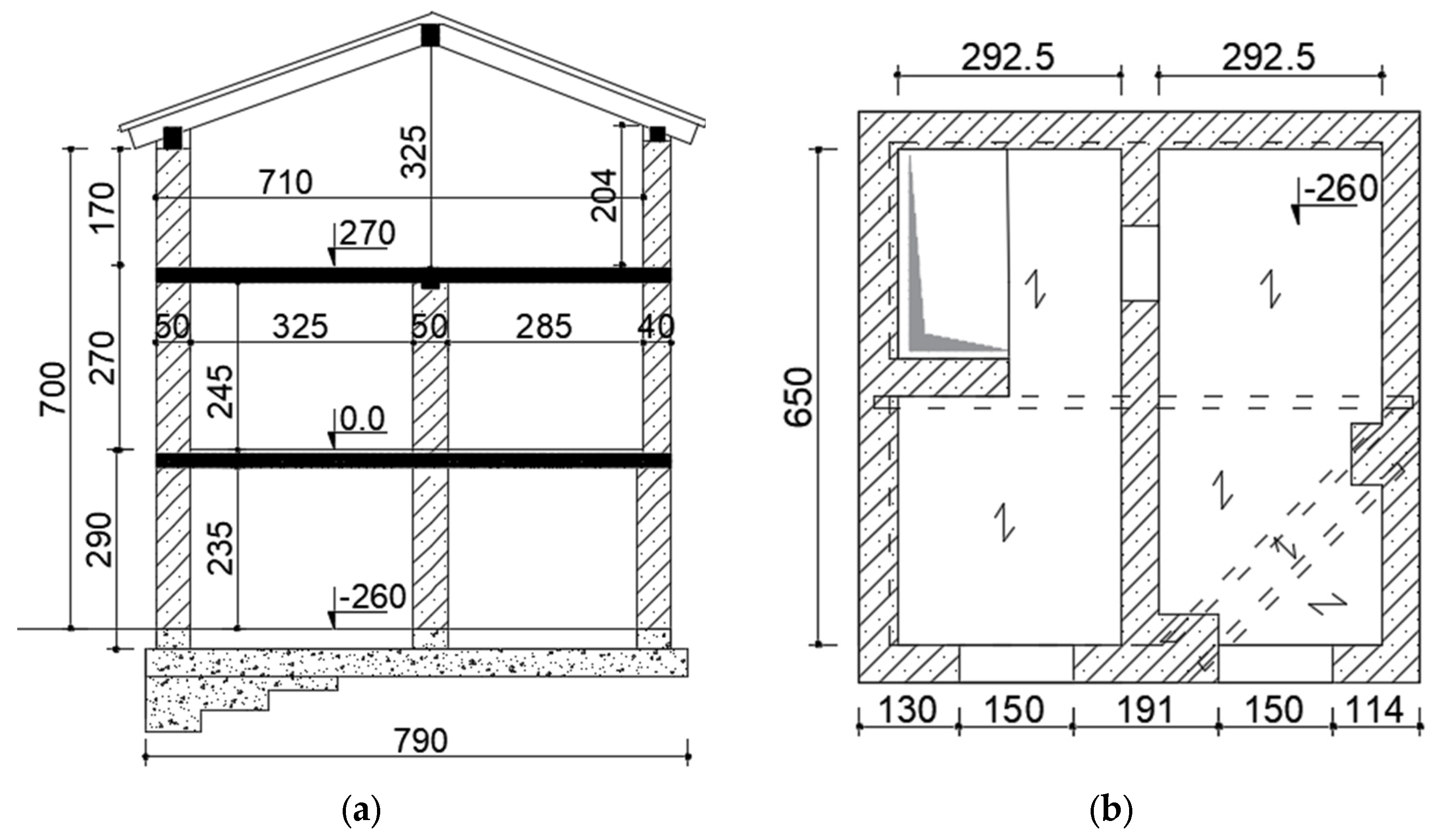
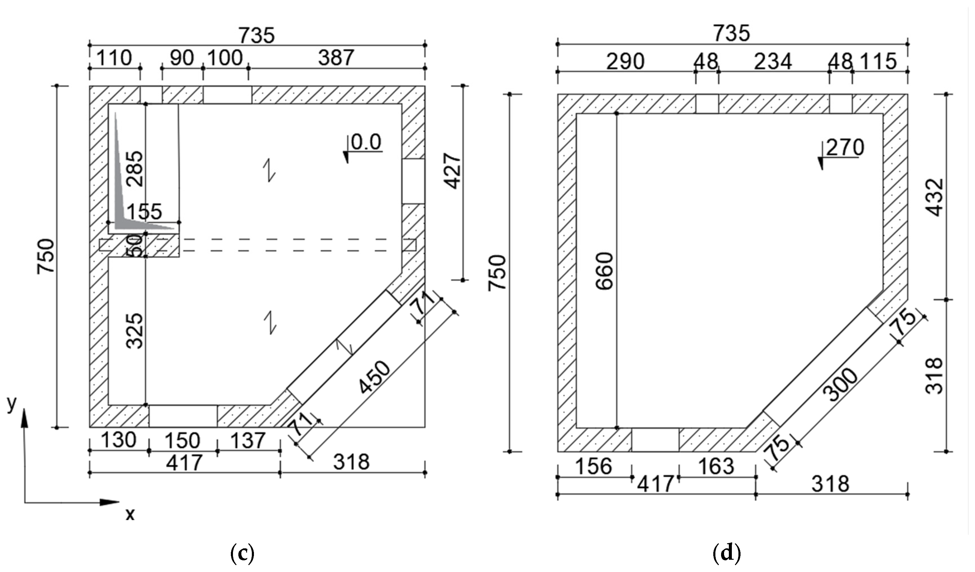
. The construction plans are shown in Figure 3.
The analyzed masonry building is modeled using the equivalent frame method, implemented in 3Muri software by S.T.A. DATA (release 13.9.0.1). The mesh is represented in Figure 2b. Piers and spandrels are connected by rigid nodes; the slab is modeled as a two-way orthotropic membrane, and the roof is considered a nonstructural element (Zarzour et al. [26]).
Two models are adopted for the wall elements. In the first part of this analysis (results in Section 4.2), the masonry walls (piers and spandrels) are modeled as beam-elements (Lagomarsino et al. [30]) having elasto-perfectly-plastic behavior. This model is implemented in the 3Muri software. In the second part of the analysis (results in Section 4.3), the macro-element proposed by Penna et al. [32] is adopted, as implemented in the research version (TREMURI, release 2.5.0) of the software. This macro-element more appropriately reproduces the dissipation in a dynamic analysis, compared to a beam model (Bracchi et al. [40]). In fact, the hysteresis curves obtained experimentally by a cyclic pushover test in a masonry wall (e.g., Anthoine et al. [41]) are reproduced conveniently using the numerical model proposed by Penna et al. [32].
A measurement campaign, undertaken using velocity sensors placed inside the building, provides the structural response under ambient vibration (Zarzour et al. [26]), allowing for the estimation of dynamic properties in elastic conditions by operational modal analysis (Brincker et al. [42], Brincker and Ventura [43] and Michel et al. [44]). As the building is unoccupied, for the comparison of numerical and operational modal analysis, the dead load is estimated to be equal to 10   kg / m 2 for the first and second floor and 70   kg / m 2 for the roof.
The low-strain damping of the building is estimated using the random decrement technique applied to the structural response to ambient vibration (Cole [45]), and then the damping ratio ζ = 1.5 % (Zarzour et al. [26]) is adopted in the following computations.
The adopted model validation approach consists of comparing the dynamic features of the building, obtained by numerical and operational modal analysis. In particular, the first three natural frequencies are estimated for both 3D building models and compared with those obtained by the inversion of measured velocity time histories. The natural frequency is proportional to the stiffness-to-mass ratio. In the building model, the geometry, the applied vertical loads and material density influence the mass; the geometry and mechanical parameters of materials impact the stiffness. Since the geometry of the building is reasonably known and the building is unoccupied, the uncertainty of the building mass is negligible. Consequently, the natural frequencies are mostly influenced by the elastic modulus in compression of masonry structural elements, which is the only calibrated parameter. In fact, the shear modulus is assumed as G = 0.4   E (Table 1), according to Eurocode 6 [39].
After having validated the match of the fundamental frequency, if the set of sequential natural frequencies of the masonry building is not properly reproduced it means that the model must be corrected in terms of stiffness distribution. In masonry buildings with timber floors, the connection between walls and the horizontal diaphragm, as well as the choice of mechanical parameters for the orthotropic diaphragm, strongly influence the natural frequencies. Moreover, natural frequencies are impacted by the imposed position of the slab with respect to the beams, because the equivalent frame idealization is modified based on it (Zarzour et al. [26]). In fact, the second natural frequency is better reproduced considering the correct slab position ( 10   cm above the beam centroidal axis) and using the wood mechanical parameters related to the strength class of the timber (GL24h) for joists and planks. The same timber slab configuration is adopted for both 3D building models.
The building model with beam-elements is considered validated because of the match of the first three natural frequencies (Table 2), obtained using an elastic modulus in compression of the masonry E = 3750   MPa , which are slightly higher than that obtained by the compression test on triplet masonry specimens (Table 1). The frequency discrepancy f i N M A f i O M A / f i O M A , with i = 1 , 2 , 3 , is estimated considering the OMA as the reference (Table 2). The interested reader can refer to Zarzour et al. [26] for the comparison of mode shapes, in the case of the equivalent frame model with beam-elements.
The comparison of the numerical and operational modal analysis in the case of the building model with macro-elements allows for the calibration of the elastic modulus in compression, which results in E = 4500   MPa . The lower stiffness of the macro-element, compared to the beam-element, implies a higher elastic modulus to attain the measured natural frequencies. This is consistent with the discussion made by Beyer et al. [44] about the decrease in the elastic moduli in the building model with beam-elements to allow for a fair comparison with the model using macro-elements. The first three natural frequencies and the effective masses estimated using the macro-element model are listed in Table 2. The first and the second mode represent a translational mode in the x- and y-direction (Figure 3), respectively, and the third mode is torsion.
After calibrating the elastic modulus in compression E , a live load has been added ( 200   kg / m 2 on each floor and 170   kg / m 2 on the roof) for the following analyses, according to the building design process. First, a pushover analysis is performed using the 3D equivalent frame model with beam-elements, and the pushover curves F , U are obtained, representing the base shear strength versus the average top floor displacement weighted based on nodal mass as proposed by Galasco et al. [31]. The pushover curves are truncated at the ultimate displacement U u . Based on a risk-targeted safety approach, the ultimate displacement U u is defined as the displacement corresponding to the failure of the first pier element, coherently with the analyzed limit state. The near collapse limit state for the pier is considered attained when the drift exceeds the threshold of 0.4 % in shear and 0.8 % in bending. These values are proposed in the EC8 [34]. Then, four mechanical parameters of the macro-element proposed by Penna et al. [32] are calibrated in an attempt to reproduce the base shear force at the plateau of the bilinear pushover curve obtained for the equivalent frame model with beam-elements. In particular, two pushover curves (uniform load distribution in the x- and y-direction according to the coordinate system in Figure 3), displayed in Figure 4, are selected to calibrate the parameters. Since a reduction factor for the ultimate compressive strength of masonry 0.85   f ¯ is taken into account in the formulation of the strength domain adopted for the beam-element for flexure failure (Magenes and Della Fontana [46]), according to an equivalent rectangular stress block [34], this factor is considered also in the macro-element model to ensure consistency with the beam-element (Penna et al. [32], Beyer et al. [44]).
In a first attempt, the equivalent pure shear strength f v 0 * and equivalent friction coefficient tan φ * of the macro-element are assumed equal to the corresponding masonry properties f v 0 and tan   φ in Table 1) used in the beam model (Zarzour et al. [26]). In this way, the plateau of the pushover curves for the equivalent frame model with macro-elements, in x- and y-direction, appear higher than the corresponding ones obtained using the beam-element, for the same material properties. Consequently, f v 0 * and tan φ * are obtained by calibration, in each direction, reducing their value until reproducing the base shear force at the plateau of the bilinear pushover curve obtained for the equivalent frame model with beam-elements (Figure 4). Thus, the equivalent shear mechanical parameters adopted for the macro-element, f v 0 * = 0.092   MPa and tan   φ *   =   0.1 in x-direction, f v 0 * = 0.082   MPa and tan   φ * = 0.1 in y-direction, are significantly lower than the corresponding material properties f v 0 = 0.26   MPa and tan   φ = 0.4 used in the beam model (Zarzour et al. [26]). This is coherent with the results discussed in the literature for the adopted macro-element (Penna et al. [32,47]).
In addition, two other model parameters, G c t and β , must be calibrated for the macro-element, according to Penna et al. [32]. They are assumed as G c t = 1 and β = 0 with the same goal of approximating the elastic perfectly plastic behavior obtained for the equivalent frame model with beam-elements (same value of the base shear force at the plateau of the pushover curve).
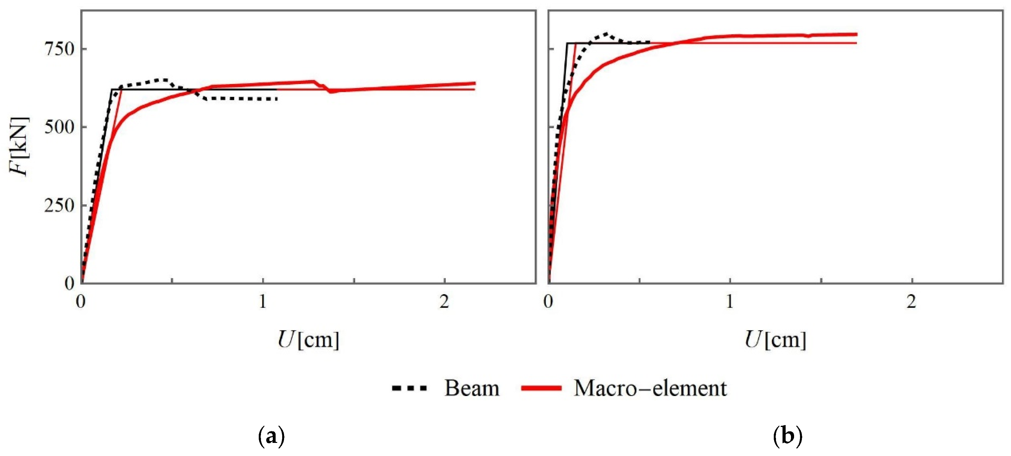
In Figure 4, the pushover curves obtained using the 3D building model with macro-elements or beam-elements are represented for the case of uniform load distribution in the x- and y-direction (coordinate system in Figure 3) neglecting an accidental eccentricity. The model validation in elastic conditions is confirmed by the similarity of the initial slope in the pushover curve for both elements. Then, the bilinear idealization of the pushover curve is obtained by imposing an initial stiffness corresponding with F = 0.7   F max (Tomaževič [6]) in each curve (see Section 2). The first slope of the bilinear curve is lower (reduced stiffness) in the case of the macro-element compared with that for the beam-element. In fact, using the macro-element the stiffness reduction caused by progressive cracking is modeled; consequently, the secant stiffness varies more before attaining the plateau in the pushover curve. Whereas, when the beam-element is used, any decrease in stiffness is attributed only to the yielding of elements (Beyer et al. [48]). From the bilinear curve, the ductility capacity μ c = U u / U y is calculated and the overstrength ratio O S R = F y / F y 1 is determined (Table 3). As shown in Figure 4, for both loading directions, the ductility capacity μ c is significantly higher when using the macro-element rather than the beam-element in the equivalent frame model, even if the same collapse criterion is adopted in both cases in terms of drift limit. This difference can be justified by the fact that the drift definition is not the same for both elements: two drifts are defined for the macro-element, for flexural and shear response, and each one is compared to the corresponding drift limit; instead, a single drift is calculated in the beam-element and compared to the limit related to the damage mechanism (Lagomarsino et al. [30], Penna et al. [32]). In addition, as presented in Penna et al. [49], for the same top displacement, the drift is higher in the beam-element compared to the flexural and shear drift in the macro-element, leading to an earlier attainment of the local ultimate condition and a lower global displacement capacity.
Afterwards, the related capacity curve for an equivalent SDOF system is derived scaling the pushover curve (the participation factor Γ is the scaling constant) and it is idealized into a bilinear curve. The yield displacement u y , ultimate displacement u u and yield force f y are presented in Table 4 for the equivalent SDOF system having mass m 0 and the natural period T 0 = 2 π   m 0   u y / f y . Since the slope of the bilinear curve u y , f y is different for the two models, the natural period T 0 of the equivalent SDOF system does not coincide.

4. Comparison of FRF Estimation Methods

This research aims to compare the demand-based (DB), capacity-based (CB) and capacity-demand-based (CDB) methods for the FRF estimation, discussed in Section 2. In the first part of this analysis, the pushover curve is obtained using the 3D building model in which the wall elements are modeled by beam-elements (dashed line in Figure 4) and the FRF estimation for the three methodologies is performed using an equivalent SDOF system to reduce the computation time of dynamic analysis. In the second part of this analysis, the pushover analysis (thick solid line in Figure 4) and the FRF estimation according to the CB-approach are both carried out using the 3D building model. In this case, the wall elements are modeled as macro-elements because they more appropriately reproduce the dissipation in a dynamic analysis, compared to a beam model. These results are compared with the CDB-FRF.
One hundred synthetic signals are generated according to Cacciola et al. [33] and the guidelines of Eurocode 8 [27] about the damping ratio 5 % , the strong motion duration (selected as 10   s ) and the total duration (selected as 25   s ). Their compatibility with the elastic response spectrum of Eurocode 8 [27] is verified according to the criteria defined in the same code. Moreover, a different number of signals is considered in order to evaluate its effect on the results in terms of FRF and the spectrum compatibility is verified for a set of fifteen, thirty and fifty signals. The comparison between the mean response spectrum for fifteen synthetic acceleration time histories and the target elastic response spectrum [27] is shown in Figure 5.

4.1. FRF Estimation Using a SDOF System

The three methodologies for the FRF estimation, namely the DB-, CB- and CDB-method (Section 2), are first compared in the case where the structure is represented by an equivalent SDOF system in the dynamic analysis. Accordingly, the pushover curve shown in Figure 4 (dashed line), for the 3D building model with beam-elements, is scaled to obtain the related capacity curve for the equivalent SDOF system. This capacity curve is idealized by a bilinear curve, whose parameters are indicated in Table 4. The structure is modeled as an equivalent SDOF system having natural period T 0 = 2 π   m 0   u y / f y (Table 4) and the estimated building damping ratio ζ = 1.5 % .
The DB-FRF (ratio between the base shear forces in elastic and elasto-plastic conditions) is calculated as q 0 = f e / f y , where the base shear force f e is obtained as the maximum base shear attained during dynamic analysis, in elastic conditions, using as seismic load an acceleration time history of the set of one hundred synthetic spectrum-compatible accelerograms (seismic demand). The yield base shear force f y is the plateau of the bilinear capacity curve (Table 4).
The CB-FRF is calculated using the same formulation, q 0 = f e / f y , but the base shear force f e is estimated for a seismic load amplitude related to the ultimate displacement (system capacity). In fact, the elastic force f e is the maximum base shear attained during dynamic analysis, in elastic conditions, using as seismic load an acceleration time history of the same set of one hundred synthetic spectrum-compatible accelerograms but scaled to increase the peak amplitude with the aim of attaining the ultimate displacement. The scaling factor is determined by an IDA, using the bilinear capacity curve of the building as the first-loading curve for the equivalent SDOF system.
The CDB-FRF is deduced from a ductility-FRF curve, corresponding with the building ductility capacity μ c (Table 3). A ductility-FRF curve is obtained by fixing a range of FRFs, and for each value the ductility demand μ d = u max / u y is calculated after a dynamic analysis in elasto-plastic conditions, using as seismic load one of the one hundred synthetic spectrum-compatible accelerograms representing the seismic demand (ensuring that q 0 d 1 , as in Equation (7)).
The three methodologies provide the FRF on a statistical basis because a different value is obtained for each seismic signal.

4.2. Comparison of FRF Estimation Methods Using a SDOF System

The DB-, CB- and CDB-method are compared in the case where the structure is represented by an equivalent SDOF system in the dynamic analysis. The computation is carried out for one hundred synthetic seismic signals. The FRF is estimated for each signal and the results are represented in Figure 6 in terms of the mean FRF (symbol), and the range of values within one standard deviation is indicated.
In the DB-approach, the variability of the seismic demand implies a variation in the DB-FRF but also in the ductility demand μ d (Figure 6). The DB-FRF is more conservative because it is dependent on the ductility demand which is lower than the building ductility capacity.
The CB- and CDB-approaches deduce the FRF as related to the ductility capacity of the building ( μ c = 6.37 in Table 3). The CDB-method is more efficient in terms of computation time, compared with the CB-approach. The obtained average ductility-FRF curve is represented in Figure 6a and the CDB-FRF is deduced from this curve (indicated by the symbol x), as proposed by Zarzour et al. [26].
The range of the ductility-FRF curves is shown in Figure 6b (gray zone), obtained for the same SDOF system characterized by the natural period and viscous damping. Each point of a ductility-FRF curve is obtained for a fixed FRF. Consequently, for each FRF q 0 , the variability of the curves is associated with the estimation of the ductility attained for each input ground motion. If a value of the FRF is obtained from each curve, a narrow dispersion appears and the mean FRF is indicated (symbol x) in Figure 6b. The difference in terms of mean FRF is negligible if the FRF is deduced from the average ductility-FRF curve as related to the ductility capacity (Figure 6a) or if the mean FRF is obtained for the set of curves (Figure 6b).
As displayed in Figure 6, the CB-method provides a much higher mean FRF, with a higher dispersion of results. This dispersion can be influenced by the variability of the PGA in the set of seismic signals (see Figure 7). The higher mean FRF could be due to the use of the equivalent SDOF approximation in the IDA, as discussed in Section 4.3.
Furthermore, the FRF is calculated as the PGA ratio in ultimate and yielding conditions q 0 = P G A u / P G A y , as discussed by Milosevic et al. [35], using the formulation of the structure top displacement according to the N2 method (Equation (2)) and its correction for masonry structures (Equation (4)). The mean FRF obtained by the CDB-method is consistent with the N2-based approaches.
In DB- and CDB-approaches, synthetic spectrum-compatible acceleration time histories are used and the PGA is strictly related to the prescribed seismic demand. Consequently, the PGA variability is very low, only due to the generation process of random spectrum-compatible synthetic signals. Moreover, as the same set of seismic signals is used for the DB- and CDB-approaches, the same statistics are obtained in terms of PGA (Figure 7). On the other hand, in the CB-approach, the variability of the PGA is higher because it is related to the building collapse defined as ultimate top displacement. In fact, in this case, the PGA associated with the ultimate top displacement, deduced through a nonlinear IDA, depends on the input time history.
The low PGA variability in the DB-approach yields a narrow dispersion of results in terms of the FRF, as shown in Figure 7. When the CDB-method is adopted, the variability of the FRF (Figure 7) appears if one FRF is deduced from the ductility-FRF curve obtained for each generated signal (as in Figure 6b). As mentioned before, the CB-method provides a higher dispersion of results in terms of the FRF, and this seems be associated with the high PGA variability. A higher PGA leads to a greater elastic base shear force f e , without modifying f y , resulting in a higher CB-FRF.
The sensitivity of FRF statistics to the number of samples and, as a consequence, to the number of seismic signals is investigated and is displayed in Figure 8 for the CB- and CDB-FRF. In this analysis, fifteen signals are enough for both approaches even if the CB-FRF is more sensitive to the adopted number of signals. This is coherent with the analysis performed by Mohsenian et al. [20].
The relationship of the FRF with the damping ratio, as well as with the ductility capacity, is investigated using the CDB-method. The results are obtained for a natural period T 0 = 0.12   s (Table 4). The FRF increases with the ductility capacity for a given building damping ratio, as displayed in Figure 9a for three damping ratios. A higher damping ratio reduces the attained ductility (ultimate displacement) for a given FRF and seismic demand, and consequently the ductility-FRF curve has a softer slope (Figure 9a); consequently, for a given ductility a higher damping ratio yields a higher FRF, but the variation in the FRF with the damping ratio seems slight. The trend of FRF increase with the building damping ratio is represented in Figure 9b for a given ductility capacity of the building. It is similar for the three ductility levels.
The dependence of the FRF on the natural period is examined using the CB- and CDB-method (Figure 10). The FRF increases with both the ductility capacity and the natural period of the structural system, in accordance with the results presented by Chopra [12].
As already discussed for the results shown in Figure 6, the CB-method provides higher values of the FRF compared with the CDB-method when using an equivalent SDOF system. In the next section, the CB-method is applied to the 3D model of the building, selected as a reference, to verify the estimation of the FRF by the different simplified approaches.

4.3. FRF Estimation Using a 3D Building Model

In this section, the CB-approach for the FRF estimation (Section 2) is applied in the case where the structure is represented by a 3D model in the linear and nonlinear dynamic analyses, carried out using the TREMURI research version (release 2.5.0). The CDB-method is applicable only for an equivalent SDOF system, but it is considered for the comparison of results.
As discussed in Section 3, the equivalent frame model with the macro-element developed by Penna et al. [32] is adopted because of its better reproduction of energy dissipation compared with a beam-element. Accordingly, the bilinear idealization of the pushover curve for the building model with macro-elements, represented in Figure 4, is used to define the yield base shear force F y . The FRF estimation is performed using the set of fifteen synthetic spectrum-compatible seismic signals (Figure 5 and Figure 8) to reduce the number of dynamic analyses. The analyses are carried out in the x- and y- direction.
The hysteretic curves (base shear force versus top floor lateral displacement) obtained by simulating the structural response using an equivalent SDOF system and a 3D building model are presented in Figure 11. These curves are obtained for compatible seismic signals scaled to achieve the ultimate displacement U u attained in the pushover analysis performed for the 3D building model in x-direction (the first three signals in Table 5). The behavior of the equivalent SDOF system is assumed as elastic-perfectly-plastic and therefore the first-loading curve is bilinear (Vidic et al. [16], Borzi and Elnashai [50] and Chopra [12]). The unloading phase has the same slope as the initial one.
In the CB-method, the PGA is obtained by IDA (Section 2) to match the building ultimate displacement. The results are listed in Table 5 for the set of fifteen seismic signals, in both cases of dynamic analysis for the equivalent SDOF system and the 3D building model, in the x- and y-direction. When the 3D building model is used, the target ultimate displacement U u is the last point of the pushover curve. Whereas, when an equivalent SDOF system is considered, the ultimate displacement u u is obtained from the capacity curve. For this reason, the PGA values obtained for the equivalent SDOF system are multiplied by the participation factor ( Γ = 1.02 in x-direction and Γ = 0.84 in y-direction, as indicated in Table 4). The mean PGA (Table 5) is significantly higher when the dynamic analysis is performed for the equivalent SDOF system compared to the 3D building model.
The N2 method (Fajfar [17]) and its correction proposed by Guerrini et al. [18] allow for the estimation of the PGA related to the ultimate displacement u u (displacement capacity) if it is considered as displacement demand u d in Equations (2) and (4), respectively. The displacement capacity u u is obtained starting from the pushover curve associated with the 3D building model with macro-elements (Figure 4, Table 3 and Table 4). The PGA values obtained for the equivalent SDOF system using the N2 method and its correction are also multiplied by the participation factor ( Γ = 1.02 in x-direction and Γ = 0.84 in y-direction as indicated in Table 4). As indicated in Table 5, the correction of the N2 method proposed by Guerrini et al. [18]) provides a PGA closer to the mean value obtained using the 3D building model in the dynamic analysis, for both the x- and y-direction. This correction is proposed for masonry structures characterized by a short natural period < T C , as is the case of the analyzed building (equivalent natural period T 0 = 0.1391   s in the x-direction and T 0 = 0.1007   s in y-direction, as reported in Table 4).
Previous studies on the behavior factor (Fajfar [11]) observe a moderate influence of hysteretic structural behavior in the whole period region. In the CDB-method, the ductility demand is estimated using an equivalent SDOF system having elasto-perfectly plastic behavior, but the ductility estimation is performed on a statistical basis and the effect of each time history is averaged. Consequently, the only common parameter for all signals is the target PGA, and the effect of the time history is flattened.
On the contrary, when an equivalent SDOF system and a 3D building model are adopted in the CB-method, the different energy dissipation model for both systems (represented in Figure 11 as hysteresis curves) implies an important difference in the PGA estimated by IDA (related to the building ultimate displacement). The calibration of the PGA yielding the attainment of the ultimate displacement is strongly dependent on the time history, and the different hysteresis dissipation for each time history (Figure 11) influences the obtained PGA (Table 5). A significant overestimation of the PGA is obtained when using the equivalent SDOF system with elasto-perfectly-plastic behavior in the IDA, instead of the 3D building model with macro-elements.
The comparison of hysteretic curves obtained by simulating the structural response using a 3D building model shaken in the x-direction, in the case of the dynamic analysis in linear elastic and elasto-plastic conditions, is presented in Figure 12 for the same three signals, scaled to achieve the ultimate displacement U u attained in the pushover analysis performed for the 3D building model (the first three signals in Table 5).
The FRF estimated using the CB-method in the case of equivalent SDOF system and 3D building model are listed in Table 6 for the set of fifteen scaled seismic signals (Table 5) imposed in the x- and y-direction. As expected, the CB-FRF obtained using the seismic signals scaled by IDA using the equivalent SDOF system are significantly higher, because the elastic base shear force F e is proportional to the PGA, which is higher in this case (see Table 5).
As a test, the seismic signals scaled using the IDA, related to the ultimate displacement for the 3D building model (Table 5), are used as input at the base of the equivalent SDOF system in the dynamic analysis. In this case, the obtained mean FRF is q 0 = 3.89 in the x-direction and q 0 = 2.61 in the y-direction. These values are very close to the mean FRF obtained by performing the dynamic analysis using a 3D building model shaken by the same set of seismic signals ( q 0 = 3.90 in the x-direction and q 0 = 2.21 in the y-direction, in Table 6). This means that the difference in the results obtained using the CB-approach for an equivalent SDOF system and a 3D building model (Table 6) are associated with the estimation of the PGA related to the building capacity as a consequence of the energy dissipation model used for both systems (Figure 11). In fact, using the same ground motion amplitude, the difference between the dissipation models is eliminated because the yield shear force is deduced from the pushover curve and then the elastic maximum base shear force is estimated in the linear elastic regime.
The FRF calculated as the PGA ratio in ultimate and yielding conditions q 0 = P G A u / P G A y , as discussed by Milosevic et al. [35]), is added in Table 6, where the PGA is deduced from the displacement of the equivalent SDOF system calculated according to the N2 method (Equation (2)) and its correction (Equation (4)).
Then, the CDB-FRF is compared with the CB-FRF obtained using a 3D building model which is considered as a reference (Table 6). The mean FRF is deduced first from the average ductility-FRF curve for the fixed ductility capacity (Zarzour et al. [26]), as in Figure 6a (zero standard deviation), and then as the mean FRF for the set ductility-FRF curves, each curve associated with a different seismic signal (Figure 6b). Both values are indicated in Table 6. Since in the y-direction the target load ratio is q 0 d = 0.86 < 1 (Table 4), as explained in Section 2.4, the amplitude of the seismic signals in this direction is increased to attain q 0 d = m 0   S e T 0 / f y = 1 and avoid an overestimation of the FRF.
Moreover, the CDB-FRF obtained by the average ductility-FRF curve is represented in Figure 13 and compared with the CB-FRF estimated using the 3D building model and the N2-based approaches. All the adopted formulations yield a higher FRF (Table 6) compared with the one indicated in Figure 6, because of the different pushover curves (Figure 4) adopted in the analysis.
The proposed CDB-method for the estimation of the FRF provides results that are consistent with the CB-approach applied using the 3D building model, which is considered as the reference method. The CDB-method provides reliable values of the FRF and, compared with the CB-method, it represents a more efficient tool in terms of computation time.
As already discussed (Figure 6), the mean FRF obtained by the CDB-method is consistent with the results provided by the N2-based approaches. In the analyzed cases, the CDB-method yields safe results compared with the N2 method. The discrepancy between the methods varies with the loading direction (Figure 13) and load distribution.
As mentioned in Section 2.3, the corrected N2 approach (Guerrini et al. [18]) depends on four parameters calibrated specifically for typologies of masonry structures, according to the hysteretic behavior associated with the different damage mechanisms observed in the masonry structure. In particular, the coefficients adopted in this analysis are provided for masonry buildings presenting shear-dominated dissipation. It is worth noting that the proposed CDB-method does not present restrictions concerning the construction material and structural typology (except the requirement of a dominant first mode shape to ensure the SDOF system is representative), and any calibration of parameters is required in the structural model if a bilinear capacity curve is used. Moreover, in the CDB-method, the ductility-FRF curve is obtained numerically for the building natural period instead of imposing a general analytical FRF-ductility-period relationship.
The FRF values in Table 6 are obtained for the case study and only two load combinations, with the aim of comparing different approaches for the FRF estimation, and cannot be considered as reference values for any rubble stone masonry building.

5. Conclusions

This research compares three methodologies for estimating the behavior factor of a building, mainly related to the force reduction factor (FRF), which is used for the seismic design of the bearing structure. The analysis of the FRF estimation is performed for a rubble stone masonry building, modeled using the equivalent frame approach. Nevertheless, the three methods can be applied to other typologies of building structures and construction materials.
The FRF is obtained using a so-called capacity-demand-based (CDB) method previously proposed by the authors. This CDB-method provides a ductility-FRF curve obtained by estimating the ductility attained during a seismic event reproduced using a synthetic spectrum-compatible accelerogram (ductility demand) under the assumption that the structure has an elastic behavior until the yield top displacement related to the design load and a fixed FRF. This ductility-FRF curve is used to deduce the FRF related to the ductility capacity of the building. The proposed methodology for the FRF estimation is compared with other approaches discussed in the literature. The demand-based (DB) method estimates the FRF as the linear elastic to nonlinear (elastic-perfectly plastic) maximum base shear force ratio, in which the maxima are attained during a seismic event represented using a synthetic spectrum-compatible accelerogram. This estimation is performed on a statistical basis. According to the capacity-based (CB) method, the same definition of the FRF is adopted, but the maxima are attained during a synthetic acceleration time history scaled in such a way that the peak ground acceleration is related to the building ultimate displacement. The scaling constant is obtained by IDA.
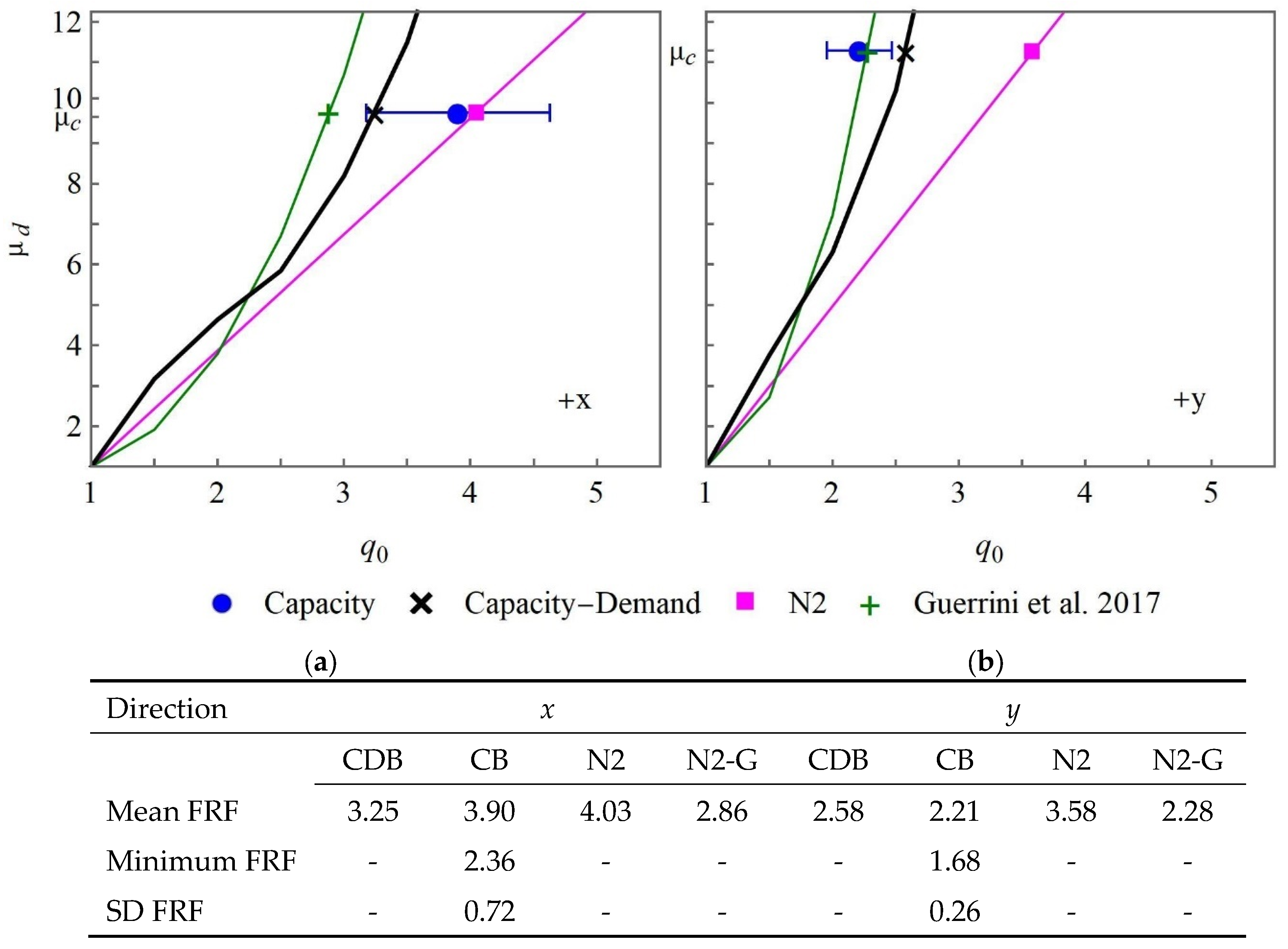
The three approaches are adopted for an equivalent SDOF system to reduce the computation time. On the other hand, the CB-FRF is estimated by performing the dynamic analyses for a 3D building model. As expected, the DB-approach underestimates the FRF when the building capacity is not attained. On the other hand, the CB-FRF is overestimated when a SDOF system is used in the IDA for the scaling of seismic signals used as input. In this context, the CDB-method yields results which are consistent with those obtained by the CB-method using a 3D building model, with a reduced computation time, and provides safe values compared with the N2 method. Moreover, the results obtained using the CDB-method are consistent with the FRF estimated using the corrected N2 method proposed by Guerrini et al. [18] specifically for masonry buildings. The discrepancy between the methods varies with the loading direction and load distribution.
It is worth noting that the proposed CDB-method does not present restrictions concerning the construction material and structural typology (except the requirement of a dominant first mode shape to ensure that the SDOF system is representative) and any calibration of parameters is required in the structural model if a bilinear capacity curve is used. In the CDB-method, the ductility-FRF curve is obtained numerically for the building natural period instead of imposing an analytical FRF-ductility-period relationship.
In conclusion, the proposed CDB-method for the FRF estimation is verified by comparison with other approaches presented in the literature and provides a reliable estimation of the FRF, close to the values obtained using the CB-approach applied to a 3D building model that is considered as a reference. The reduced computation time legitimizes considering it as an efficient tool for professional practice, without restrictions on construction material and structural typology.
The reliability of the proposed CDB-method is demonstrated for masonry buildings characterized by a short natural period. Further research is necessary to verify the results in the range of long periods. Moreover, when the first two translational mode shapes are not dominant (high effective mass), the assumption of an equivalent SDOF system is not suitable and the equivalent system must be adapted.

Author Contributions

Conceptualization, N.Z. and M.P.S.d.; methodology, N.Z. and M.P.S.d.; software, N.Z. and M.P.S.d.; validation, N.Z. and A.P.; formal analysis, N.Z. and M.P.S.d.; investigation, N.Z. and M.P.S.d.; resources, M.O. and M.P.S.d.; data curation, N.Z.; writing—original draft preparation, N.Z. and M.P.S.d.; writing—review and editing, N.Z. and M.P.S.d.; visualization, N.Z. and M.P.S.d.; supervision, M.P.S.d. and L.L.; project administration, M.P.S.d.; funding acquisition, M.P.S.d., M.O. and L.L. All authors have read and agreed to the published version of the manuscript.

Funding

This research is carried out in the framework of the French National Project “Mechanical behavior of compressed earth blocks for sustainable building construction in seismic areas” (DYNATERRE, ANR-23-CE04-0015-01) funded by the French National Research Agency. This work has been funded by the region SUD (South-Eastern France) and by the FILIATER company through a doctoral fellowship. Moreover, the FILIATER company funded the experimental campaign (laboratory data and ambient vibration recording campaign).

Data Availability Statement

The research data and code are available but not shared because they are produced in the framework of a current national research project (DYNATERRE, ANR-23-CE04-0015-01) with a group of research institutions and private companies. The data can be shared in accordance with the consortium agreement.

Acknowledgments

The authors thank Stefano Bracchi for his fruitful help with the TREMURI research version.

Conflicts of Interest

The authors declare that they have no competing financial interests or personal relationships that could influence the work reported in this paper.

References

  1. Bocciarelli, M. On the behavior factor of masonry towers. Soil. Dyn. Earthq. Eng. 2017, 101, 81–89. [Google Scholar] [CrossRef]
  2. Hummel, J.; Seimb, W. Displacement-based design approach to evaluate the behaviour factor for multi-storey CLT buildings. Eng. Struct. 2019, 201, 109711. [Google Scholar]
  3. Aloisio, A.; Alaggio, R.; Fragiacomo, M. Fragility functions and behavior factors estimation of multi-story cross-laminated timber structures characterized by an energy-dependent hysteretic model. Earthq. Spectra 2020, 37, 134–159. [Google Scholar] [CrossRef]
  4. Gubana, A.; Mazelli, A. Evaluation of the Behaviour Factor by Incremental Dynamic Analysis for the Seismic Design of Light-Frame Timber Buildings. In Proceedings of the World Conference on Timber Engineering, Oslo, Norway, 19–22 June 2023. [Google Scholar]
  5. Uang, C. Establishing R. (or Rw) and Cd factors for building seismic provisions. J. Struct. Eng. 1991, 117, 19–28. [Google Scholar] [CrossRef]
  6. Tomaževič, M. Earthquake-Resistant Design of Masonry Buildings; Imperial College Press: London, UK, 1999. [Google Scholar]
  7. Tomaževič, M.; Bosiljkov, V.; Weiss, P. Structural Behaviour Factor for Masonry Structures. In Proceedings of the 13th World Conference on Earthquake Engineering, Vancouver, BC, Canada, 1–6 August 2004. Paper No. 2642. [Google Scholar]
  8. Blume, J.A. Allowable Stresses and Earthquake Performance. In Proceedings of the 6th World Conference on Earthquake Engineering, New Delhi, India, 10–14 January 1977; pp. 165–174. [Google Scholar]
  9. Morandi, P. New Proposals for Simplified Seismic Design of Masonry Buildings. Ph.D. Thesis, Rose School, University of Pavia, Pavia, Italy, 2006. [Google Scholar]
  10. Magenes, G. Masonry Building Design in Seismic Areas: Recent Experiences and Prospects from a European Standpoint. In Proceedings of the 1st European Conference on Earthquake Engineering and Engineering Seismology, Geneva, Switzerland, 3–8 September 2006. [Google Scholar]
  11. Fajfar, P. The Story of the N2 Method; International Association for Earthquake Engineering: Tokyo, Japan, 2021. [Google Scholar]
  12. Chopra, A.K. Dynamics of Structures: Theory and Applications to Earthquake Engineering; Prentice-Hall: Upper Saddle River, NJ, USA, 2001. [Google Scholar]
  13. Priestley, M.N.J.; Calvi, G.M.; Kowalski, M. Displacement-Based Seismic Design of Structures; IUSS Press: Pavia, Italy, 2007. [Google Scholar]
  14. Veletsos, A.S.; Newmark, N.M. Effect of Inelastic Behavior on the Response of Simple Systems to Earthquake Motions. In Proceedings of the 2nd World Conference on Earthquake Engineering, Tokyo, Japan, 11–18 July 1960; pp. 895–912. [Google Scholar]
  15. Newmark, N.M.; Hall, W.J. Earthquake Spectra and Design; Earthquake Engineering Research Institute: Oakland, CA, USA, 1982. [Google Scholar]
  16. Vidic, T.; Fajfar, P.; Fischinger, M. Consistent inelastic design spectra: Strength and displacement. Earthq. Eng. Struct. Dyn. 1994, 23, 507–521. [Google Scholar] [CrossRef]
  17. Fajfar, P. A nonlinear analysis method for performance-based seismic design. Earthq. Spectra 2000, 16, 573–592. [Google Scholar] [CrossRef]
  18. Guerrini, G.; Graziotti, F.; Penna, A.; Magenes, G. Improved evaluation of inelastic displacement demands for short-period masonry structures. Earthq. Eng. Struct. Dyn. 2017, 46, 1411–1430. [Google Scholar] [CrossRef]
  19. Mwafy, A.M.; Elnashai, A.S. Calibration of force reduction factors of RC buildings. J. Earthq. Eng. 2002, 6, 239–273. [Google Scholar] [CrossRef]
  20. Mohsenian, V.; Nikkhoo, A.; Hajirasouliha, I. Estimation of seismic response parameters and capacity of irregular tunnel-form buildings. Bull. Earthq. Eng. 2019, 17, 5217–5239. [Google Scholar] [CrossRef]
  21. Hussain, N.; Alam, S.; Mwafy, A. Developments in Quantifying the Response Factors Required for Linear Analytical and Seismic Design Procedures. Buildings 2024, 14, 247. [Google Scholar] [CrossRef]
  22. Vamvatsikos, D.; Cornell, C.A. Incremental dynamic analysis. Earthq. Eng. Struct. Dyn. 2002, 31, 491–514. [Google Scholar]
  23. Saiidi, M.; Sozen, M.A. Simple nonlinear seismic analysis of R/C structures. J. Struct. Div. 1981, 107, 937–953. [Google Scholar] [CrossRef]
  24. Chopra, A.K.; Goel, R.K. Capacity-Demand-Diagram Methods for Estimating Seismic Deformation of Inelastic Structures: SDF Systems. Report PEER-1990/Pacific Earthquake Engineering Research Center; University of California Berkley: Berkeley, CA, USA, 1999. [Google Scholar]
  25. Fajfar, P. Capacity spectrum method based on inelastic demand spectra. Earthq. Eng. Struct. Dyn. 1999, 28, 979–993. [Google Scholar]
  26. Zarzour, N.; Santisi d’Avila, M.P.; Mercerat, E.D.; Lenti, L.; Oggero, M. Behavior factor estimation for seismic design of unreinforced masonry buildings. Case Stud. Constr. Mater. 2023, 19, e02483. [Google Scholar]
  27. EN 1998-1; Eurocode 8: Design of Structures for Earthquake Resistance, Part 1: General Rules, Seismic Actions and Rules for Buildings. CEN: Brussels, Belgium, 2004.
  28. Zarzour, N.; Santisi d’Avila, M.P.; Mercerat, D.; Lenti, L.; Oggero, M. Structural performance assessment of compressed earth block masonry building in seismic zone. Soil. Dyn. Earthq. Eng. 2024, 187, 108990. [Google Scholar] [CrossRef]
  29. NTC2018; Decreto Ministeriale 17 Gennaio 2018: Aggiornamento Delle «Norme Tecniche per le Costruzioni». Ministero delle Infrastrutture e dei Trasporti: Rome, Italy, 2018. (In Italian)
  30. Lagomarsino, S.; Penna, A.; Galasco, A.; Cattari, S. TREMURI program: An equivalent frame model for the nonlinear seismic analysis of masonry buildings. Eng. Struct. 2013, 56, 1787–1799. [Google Scholar] [CrossRef]
  31. Galasco, A.; Lagomarsino, S.; Penna, A. On the Use of Pushover Analysis for Existing Masonry Buildings. In Proceedings of the 1st European Conference on Earthquake Engineering and Seismology, Geneva, Switzerland, 3–8 September 2006. Paper No. 1080. [Google Scholar]
  32. Penna, A.; Lagomarsino, S.; Galasco, A. A nonlinear macroelement model for the seismic analysis of masonry buildings. Earthq. Eng. Struct. Dyn. 2014, 43, 159–179. [Google Scholar] [CrossRef]
  33. Cacciola, P.; Colajanni, P.; Muscolino, G. Combination of modal responses consistent with seismic input representation. J. Struct. Eng. 2004, 130, 47–55. [Google Scholar] [CrossRef]
  34. EN 1998-3; Eurocode 8: Design of Structures for Earthquake Resistance—Part 3: Assessment and Retrofitting of Buildings. CEN: Brussels, Belgium, 2005.
  35. Milosevic, J.; Bento, R.; Cattari, S. Seismic Behavior of Lisbon Mixed Masonry-RC Buildings With Historical Value: A Contribution for the Practical Assessment. Front. Built Environ. 2018, 4. [Google Scholar] [CrossRef]
  36. Costa, A.A.; Penna, A.; Magenes, G. Seismic Performance of Autoclaved Aerated Concrete (AAC) Masonry: From Experimental Testing of the In-Plane Capacity of Walls to Building Response Simulation. J. Earthq. Eng. 2011, 15, 1–31. [Google Scholar] [CrossRef]
  37. Official Journal of the French Republic, Decree of October 22, Arrêté du 22 Octobre 2010 Relatif à la Classification et aux Règles de Construction Parasismique Applicables aux Bâtiments de la Classe Dite «à Risque Normal», 19 October 2010. (In French). Available online: https://www.legifrance.gouv.fr/loda/id/JORFTEXT000022941755/ (accessed on 5 January 2025).
  38. International Organization for Standardization. ISO 11272; Soil Quality, Determination of Dry Bulk Density. ISO: Geneva, Switzerland, 2017.
  39. EN 1996-1-1.; Eurocode 6: Design of Masonry Structures, Part 1-1: General Rules for Reinforced and Unreinforced Masonry Structures. CEN: Brussels, Belgium, 2005.
  40. Bracchi, S.; Galasco, A.; Penna, A. A novel macroelement model for the nonlinear analysis of masonry buildings. Part 1: Axial and flexural behavior. Earthq. Eng. Struct. Dyn. 2021, 50, 2233–2252. [Google Scholar] [CrossRef]
  41. Anthoine, A.; Magonette, G.; Magenes, G. Shear Compression Testing and Analysis of Brick Masonry Walls. In Proceedings of the 10th European Conference on Earthquake Engineering, Vienna, Austria, 28 August–2 September 1995. [Google Scholar]
  42. Brincker, R.; Zhang, L.; Andersen, P. Modal identification of output-only systems using frequency domain decomposition. Smart Mater. Struct. 2001, 10, 441–445. [Google Scholar] [CrossRef]
  43. Brincker, R.; Ventura, C. Introduction to Operational Modal Analysis, 1st ed.; Wiley: Chichester, UK, 2015; pp. 1–360. [Google Scholar]
  44. Michel, C.; Guéguen, P.; Bard, P.-Y. Dynamic parameters of structures extracted from ambient vibration measurements: An aid for the seismic vulnerability assessment of existing buildings in moderate seismic hazard regions. Soil. Dyn. Earthq. Eng. 2008, 28, 593–604. [Google Scholar] [CrossRef]
  45. Cole, H.A. Online failure Detection and Damping Measurement of Aerospace Structures by Random Decrement Signatures; Report NASA CR–2205; Nielsen Engineering & Research: Santa Clara, CA, USA, 1973. [Google Scholar]
  46. Magenes, G.; Della Fontana, A. Simplified Non-Linear Seismic Analysis of Masonry Buildings. In Proceedings of the 5th International Masonry Conference, London, UK, 12–14 October 1998; pp. 190–195. [Google Scholar]
  47. Penna, A.; Senaldi, I.E.; Galasco, A.; Magenes, G. Numerical simulation of shaking table tests on full-Scale stone masonry buildings. Int. J. Arch. Herit. 2016, 10, 146–163. [Google Scholar] [CrossRef]
  48. Beyer, K.; Tondelli, M.; Vanin, F.; Petry, S.; Paparo, A. Seismic Behaviour of Unreinforced Masonry Buildings with Reinforced Concrete Slabs: Assessment of in-Plane and out-of-Plane Response; Report of the Ecole Polytechnique Fédérale de Lausanne; Bundesamt für Umwelt BAFU: Ittigen, Switzerland, 2015. [Google Scholar]
  49. Penna, A.; Rota, M.; Bracchi, S.; Angiolilli, M.; Cattari, S.; Lagomarsino, S. Modelling and seismic response analysis of existing URM structures. Part 1: Archetypes of Italian modern buildings. J. Earthq. Eng. 2022, 28, 1130–1156. [Google Scholar] [CrossRef]
  50. Borzi, B.; Elnashai, A. Refined force reduction factors for seismic design. Eng. Struct. 2000, 22, 1244–1260. [Google Scholar] [CrossRef]
Figure 1. An illustration of the definition of the force reduction factor q 0 and overstrength ratio O S R . The pushover curve and its bilinear idealization (solid line) and the linear structural response (dashed line) are represented for the same seismic load. The first significant yield is indicated with the thick point.
Buildings 15 01036 g001
Figure 2. (a) The three-story rubble stone masonry building and (b) the mesh of the equivalent frame model.
Buildings 15 01036 g002
Figure 3. Vertical section (a) and horizontal section of first (b), second (c) and third (d) level of studied 3-floor rubble stone masonry building. Dimensions are in centimeters (Zarzour et al. [26]).
Buildings 15 01036 g003aBuildings 15 01036 g003b
Figure 4. Pushover curves obtained using the 3D building model with beam-elements (dashed line) and macro-elements (thick solid line), for the uniform load distribution in the (a) x- and (b) y-direction, and the bilinear idealization of pushover curves (thin solid lines).
Buildings 15 01036 g004
Figure 5. Mean response spectrum for fifteen synthetic acceleration time histories compared with the target elastic response spectrum defined in Eurocode 8.
Buildings 15 01036 g005
Figure 6. The mean force reduction factor (FRF), and the range of values within one standard deviation (SD), estimated for a SDOF system shaken by 100 synthetic seismic signals. The applied methods for the FRF estimation are the demand-based (DB, diamond), capacity-based (CB, circle) and capacity–demand-based method (CDB, x) and the N2 method (N2, square) and the corrected N2 method (N2-G, plus) proposed by Guerrini et al. [18]. The CDB-FRF is deduced from the average ductility-FRF curve (a) and as the mean value (b) for the range of ductility-FRF curves (gray zone). The pushover curve obtained for the 3D building model with beam-elements is adopted to obtain the structural capacity parameters in all the methods.
Buildings 15 01036 g006
Figure 7. The peak ground acceleration versus the mean force reduction factor (FRF), and the range of values within one standard deviation (SD), estimated for 100 synthetic seismic signals using the demand-based (DB, diamond), capacity-based (CB, circle) and capacity–demand-based method (CDB, x).
Buildings 15 01036 g007
Figure 8. The number of seismic signals versus the mean force reduction factor (FRF) and the range of values within one standard deviation (SD), using the capacity-based (CB, circle) and capacity-demand-based method (CDB, x).
Buildings 15 01036 g008
Figure 9. (a) The ductility capacity versus the capacity-demand-based force reduction factor for a fixed damping ratio; (b) the building damping ratio versus the capacity-demand-based force reduction factor, for a fixed ductility capacity. The results are averaged for one hundred signals.
Buildings 15 01036 g009
Figure 10. Natural period (top) and ductility capacity (bottom) versus force reduction factor: (a) capacity-based and (b) capacity-demand-based estimation. Results are averaged for one hundred signals.
Buildings 15 01036 g010
Figure 11. Base shear force versus top floor lateral displacement hysteretic curves obtained simulating the building structural response using an equivalent SDOF system and a 3D model, for three ground motion signals (scaled to achieve the ultimate displacement U u attained in the pushover analysis performed for the 3D building model) applied in x-direction.
Buildings 15 01036 g011
Figure 12. The base shear force versus the top floor lateral displacement hysteretic curve obtained by simulating the building structural response to a ground motion in x-direction using a 3D model, in the case of dynamic analysis in linear elastic (bottom) and elasto-plastic (top) conditions for three seismic signals whose PGA is scaled to attain the building ultimate displacement. The pushover curve (thick line) is represented for comparison.
Buildings 15 01036 g012
Figure 13. The mean force reduction factor (FRF) and the range of values within one standard deviation (SD), estimated using the 3D building model (with macro-elements) shaken by 15 synthetic seismic signals in the (a) x- and (b) y-direction. The applied methods for the FRF estimation are the capacity-based (CB, circle) and capacity-demand-based method (CDB, x), the N2 method (N2, square) and the corrected N2 method (N2-G, plus) proposed by Guerrini et al. [18]. The CDB-FRF is deduced from the average ductility-FRF curve (solid line).
Buildings 15 01036 g013
Table 1. Mechanical parameters of stone masonry.
MasonryTest/Formula
Mass density ρ kg / m 3 2500ISO 11272 [38]
Young modulus E MPa 3100Triplet compression test
Shear modulus G MPa 1240 G = 0.4   E
Mean compressive strength f ¯ MPa 22.7Triplet compression test
Pure shear strength f v 0 MPa 0.26Shear test on couplets
Friction coefficient tan φ 0.4EC6 [39]
Tensile strength in shear f v , lim MPa 4.9 f v , l i m = 0.065   f b
f b normalized compressive strength of blocks.
Table 2. Dynamic features obtained by operational (OMA) and numerical (NMA) modal analysis. The NMA is developed using an equivalent frame model with beam- or macro-elements.
Analysis Mode 1Mode 2Mode 3
OMAFrequency [Hz]7.49.714.5
NMA Frequency [Hz]7.39.911.2
(beam-element)Frequency discrepancy [%]1222
Effective mass in x-direction [%]69.60.050.9
Effective mass in y-direction [%]0.031.30.4
NMA Frequency [Hz]7.410.412.5
(macro-element)Frequency discrepancy [%]<1714
Effective mass in x-direction [%]70.00.22.4
Effective mass in y-direction [%]0.031.10.1
Table 3. The parameters of the pushover curves obtained for a 3D building model with the wall elements modeled as beam- and macro-elements, in the case of uniform load distribution in the x- and y-direction without accidental eccentricity.
LoadWall Element F y U y U u μ c O S R
DirectionModel[kN][cm][cm]
+xBeam-element620.420.171.076.371.00
Macro-element620.650.222.169.761.38
+yBeam-element768.060.100.555.351.58
Macro-element768.860.151.6911.281.37
F y yield base shear, U y yield displacement, U u ultimate displacement, μ c ductility capacity and O S R over-strength ratio.
Table 4. The parameters of the bilinear capacity curves obtained for a SDOF system equivalent to a 3D building model with the wall elements modeled as beam- and macro-elements, in the case of uniform load distribution in the x- and y-direction without accidental eccentricity.
LoadWall Element T 0 f y u y u u μ c m 0 q 0 d Γ
DirectionModel[s][kN][cm][cm] [kg]
+xBeam-element0.1213608.250.161.056.37137,5351.361.02
Macro-element0.1391608.480.222.129.76137,4561.361.02
+yBeam-element0.0840925.380.120.665.35133,4750.860.83
Macro-element0.1007915.310.182.0111.28131,7620.860.84
T 0 fundamental period, μ c ductility capacity, f y yield base shear, u y yield displacement, u u ultimate displacement, m 0 mass, q 0 d target load ratio and Γ participation factor.
Table 5. Peak ground acceleration (PGA) obtained by IDA in x- and y-direction, related to the ultimate displacement for the equivalent SDOF system and 3D building model with macro-elements and calculated by the N2 method and corrected N2 method proposed by Guerrini et al. [18].
PGA [m/s2]
Directionxy
N° SignalSDOF3D ModelSDOF3D Model
14.904.078.135.59
27.954.217.185.38
38.944.4310.475.36
47.884.606.665.36
57.314.818.255.50
66.504.589.374.44
78.305.7911.086.61
87.694.389.095.64
98.494.628.225.45
105.794.098.664.92
115.174.937.755.98
127.674.018.305.02
138.535.157.996.24
145.854.257.875.68
159.005.0110.306.27
Mean PGA [m/s2]7.334.608.625.56
Minimum [m/s2]4.904.016.664.44
N2 [m/s2]7.318.37
N2-G [m/s2]5.225.36
Table 6. The force reduction factor (FRF) estimated for the x- and y-direction using the capacity-based method (CB), in the case of equivalent SDOF system and 3D building model with macro-elements. The CB-FRF in the case of 3D building model is considered as a reference and compared with the capacity-demand-based method (CDB), N2 method and corrected N2 method proposed by Guerrini et al. [18].
FRF
Directionxy
CB-FRFCB-FRFCDB-FRFCB-FRFCB-FRFCDB-FRF
N° SignalSDOF3D ModelSDOFSDOF3D ModelSDOF
13.973.622.515.202.292.88
27.634.432.514.722.572.48
35.742.723.295.451.682.56
49.635.403.903.972.592.22
56.904.273.645.762.312.73
65.693.713.167.652.153.03
75.953.993.335.131.962.97
84.622.363.064.362.092.36
96.953.993.725.152.082.40
105.263.712.895.382.102.94
115.174.212.264.582.432.25
126.083.392.264.771.892.99
137.424.343.613.812.262.30
145.584.052.814.252.252.45
157.994.333.737.222.522.94
Mean PGA6.313.903.25 − 3.115.162.212.58 − 2.63
Minimum3.972.363.25 − 2.263.811.682.58 − 2.22
N24.033.58
N2-G2.862.28
Disclaimer/Publisher’s Note: The statements, opinions and data contained in all publications are solely those of the individual author(s) and contributor(s) and not of MDPI and/or the editor(s). MDPI and/or the editor(s) disclaim responsibility for any injury to people or property resulting from any ideas, methods, instructions or products referred to in the content.

