The Correlation Between Crime Frequency and Urban Spatial Hierarchy in Busan

Abstract

This study examined the relationship between urban spatial hierarchy and crime rates in Busan using space syntax. This research study investigated the correlation between crime frequency and Busan’s urban space structure. The findings are as follows. Crime concentrated in areas near downtown Busan. High-control and globally integrated areas showed a strong link between city center crimes and spatial usage patterns and pedestrian routes. A weak positive correlation was found between Busan’s urban spatial hierarchy and crime frequency, indicating that urban spatial hierarchy influences crime patterns. However, the regression model’s independent variables had low explanatory power for the dependent variable, suggesting external factors influence crime occurrence beyond urban spatial hierarchy. This study provides an empirical analysis of the relationship between crime incidence and urban spatial structure in Busan, serving as essential data for future crime prevention policies.

1. Introduction

1.1. Background and Purpose

The crime rate in South Korea has risen for 10 consecutive years [1]. According to the National Police Agency, crime steadily increased from 2012 to 2022. Notably, violent crime (murder, robbery, sexual assault, larceny, and violence) increased by over 10% in 2022 compared to 2021 [2]. Although South Korea is safer than many countries, this trend highlights the urgent need for policies that enhance public safety and prevent crime [3]. The six largest metropolitan areas with high population densities report higher crime rates than other regions in South Korea [4]. This indirectly suggests that crime occurrence is closely related to a city’s size and population density. Crime within a city is generally linked to the physical environment (e.g., streetlights, surveillance cameras, and public facilities), social characteristics (e.g., income levels, unemployment rates, and social inequality), and urban structural characteristics (e.g., spatial hierarchy) [5,6,7,8,9,10]. These factors lead to differences in crime patterns across neighborhoods.

Busan, one of South Korea’s major metropolitan cities, has a crime rate that exceeds the national average [11]. As the second-largest city in South Korea, Busan has a complex urban structure comprising various spatial elements, including downtown commercial districts, residential areas, industrial and logistics zones, and ports [12,13,14,15]. The city also exhibits clear functional differentiation by region [16], with each area playing a distinct role based on its economic, social, and spatial characteristics.

According to the 2023 crime statistics from the National Police Agency, the number of crimes per 1000 inhabitants in Busan was 32.3, which surpasses the national average of 28.6, making it the city with the highest crime rate among South Korea’s metropolitan areas [17]. This phenomenon highlights the need for systematic research to analyze the factors contributing to crime in Busan. However, existing domestic studies on crime prevention and public safety management have mainly focused on other cities or specific regions, often emphasizing social and physical environmental factors [18,19,20,21,22,23]. Notably, there is a relative lack of research on urban structural characteristics, a significant factor influencing crime occurrence.

Therefore, this study examines the causal relationship between urban spatial hierarchy and crime occurrence in Busan. The findings are expected to provide practical implications for developing more effective urban planning and public safety policies. In addition, it is expected to contribute to establishing essential data for creating a safer and more sustainable urban environment and for developing crime prevention strategies.

1.2. Previous Studies

Research on crime and its spatial relationships in South Korea has been largely shaped by the Crime Prevention Through Environmental Design (CPTED) approach, developed by C. Ray Jeffery [24], and Newman’s defensible space theory [25]. CPTED focuses on reducing crime opportunities and improving safety through environmental design. This strategy is integral to urban planning and crime prevention policies, emphasizing key principles such as natural surveillance, access control, territoriality, activity support, and maintenance. Defensible space theory, conversely, links crime prevention to the physical characteristics of an area, particularly the layout and location of buildings in residential spaces.

As summarized in

Table 1. Literature review on criminal behavior and space.

Author (Year)	Purpose	Consideration Variable	Consideration of Correlation Between Crime Rates and Urban Spatial Hierarchy
Kwon (2024) [8]	To analyze the effects of spatial vulnerability awareness and residential environments on crime safety	Spatial vulnerability awareness, surveillance characteristics, and location characteristics	Not considered
Lee (2024) [9]	To analyze the importance of planning elements for the border space of apartment complexes based on a CPTED perspective	Natural surveillance, access control, territoriality, activity support, and maintenance	Not considered
Jing et al. (2024) [10]	To analyze demand for CPTED in coastal areas	Facility elements, spatial elements, and visual elements	Not considered
Kim et al. (2024) [18]	To evaluate and visualize perceived crime fear in pedestrian environments	Urban environment, fear of crime, and street images	Not considered
Oh et al. (2023) [19]	To analyze crime incidence and physical factors affecting crime from the micro- and macroperspectives	Building use, facilities, suitability, and spatial autocorrelation diagnosis	Not considered
Zhao and Kim (2022) [5]	To evaluate the safety of children’s parks in high-density cities and strategies for improving crime prevention	Social elements, safety management elements, spatial elements, and physical elements	Not considered
Kang (2022) [20]	To analyze the impact of crime prevention environmental design on safety and life satisfaction by acting as a quality-of-life component and improvement factor	Environmental elements, cultural elements, safety, and life satisfaction	Not considered
Hwang and Kang (2021) [6]	To analyze urban decline characteristics in crime-prone areas	Crime-prone areas, population decline, business decline, and deterioration of living environment	Not considered
Lee and Lee (2021) [26]	To analyze crime occurrence characteristics according to the environmental characteristics of residential streets	Environmental characteristics, facility characteristics, and spatial characteristics	Considered
Choi et al. (2020) [21]	To explore factors affecting fear of crime at the individual and regional levels	Individual variables, regional structural variables, and fear of crime	Not considered
Kim et al. (2020) [22]	To develop a model for measuring fear of crime	Emotion, cognition, and behavioral intention	Not considered
Yang (2019) [23]	To analyze CPTED applications as crime prevention strategies to improve urban safety at night	Spatial understanding, brightness distribution, color, light pollution, efficiency, and management	Not considered
Lee (2017) [7]	To conduct a correlation analysis between spatial centrality and crime	Types of crime and integration	Considered

, Kwon analyzed how spatial vulnerability awareness, crime surveillance characteristics, and location attributes influence crime safety [8]. Hwang and Kang explored the relationship between crime-prone areas and urban decline indicators, including population decline, business downturns, and deteriorating living conditions [6]. Choi et al. examined how individual factors (e.g., age, gender, and socioeconomic status) and regional structural variables (e.g., population density and security level) affect fear of crime [21]. These studies highlight the role of social factors in shaping spatial vulnerability and crime safety, demonstrating a correlation between social variables and crime occurrence.

Several studies have also focused on physical environmental factors. Lee [9] assessed the importance of the border spaces in apartment complexes from a CPTED perspective. Oh et al. assessed how physical factors—considering building usage, facilities, suitability, and spatial autocorrelation diagnostics—contributed to crime occurrence [19]. Kim et al. [22] and Yang [23] investigated how pedestrian environments influence fear of crime, analyzing CPTED elements such as spatial awareness, brightness distribution, color schemes, light pollution, efficiency, and maintenance in nighttime urban spaces. Additionally, Zhao and Kim [5], Jing et al. [10], and Kang [20] have explored crime prevention measures by considering both social and physical environmental factors. These studies examined CPTED-based user group needs relationships and reviewed factors influencing safety life satisfaction. These studies highlight the combined impact of both social and physical environmental factors on crime occurrence and their positive impact on urban planning and establishing public safety policies.

Among the previous studies, Lee and Lee [26] and Lee [7] considered the correlation between the crime rate and the urban spatial hierarchy. However, they treated urban spatial hierarchy indicators as control variables instead of primary factors. Moreover, they focused their analyses on a relatively limited scale, such as on small- and medium-sized cities and specific residential areas. Lee [7] linked urban spatial hierarchy as a control variable to crime. Their research proposed two contrasting perspectives: one suggesting that increased spatial utilization deters crime by enhancing natural surveillance and another arguing that higher population density and anonymity increase crime risks. However, Lee’s [7] study struggled to establish a direct, statistically significant link between the urban spatial hierarchy and crime rates as urban spatial hierarchy indicators were treated as control variables.

Several studies have also examined urban spatial hierarchy in Busan [27,28,29]. However, they have primarily focused on aging cities and cultural aspects. These include the location of elderly welfare facilities, museums, and potential evacuation routes for coastal disasters. Consequently, these studies differ from the present research, which explores the direct relationship between urban spatial structure and crime. Prior research has largely emphasized functional transformations in urban space rather than their direct influence on crime occurrence. This limits the ability to establish an empirical connection between urban spatial hierarchy and crime rates.

Therefore, this study empirically analyzes the relationship between the urban spatial hierarchy and crime rate in Busan. Moreover, it sets the urban spatial hierarchy indicators of control and integration as the primary independent variables. Unlike previous studies, this study quantifies the relationship between urban spatial hierarchy and crime rates in Busan.

2. Materials and Methods

2.1. Space Syntax

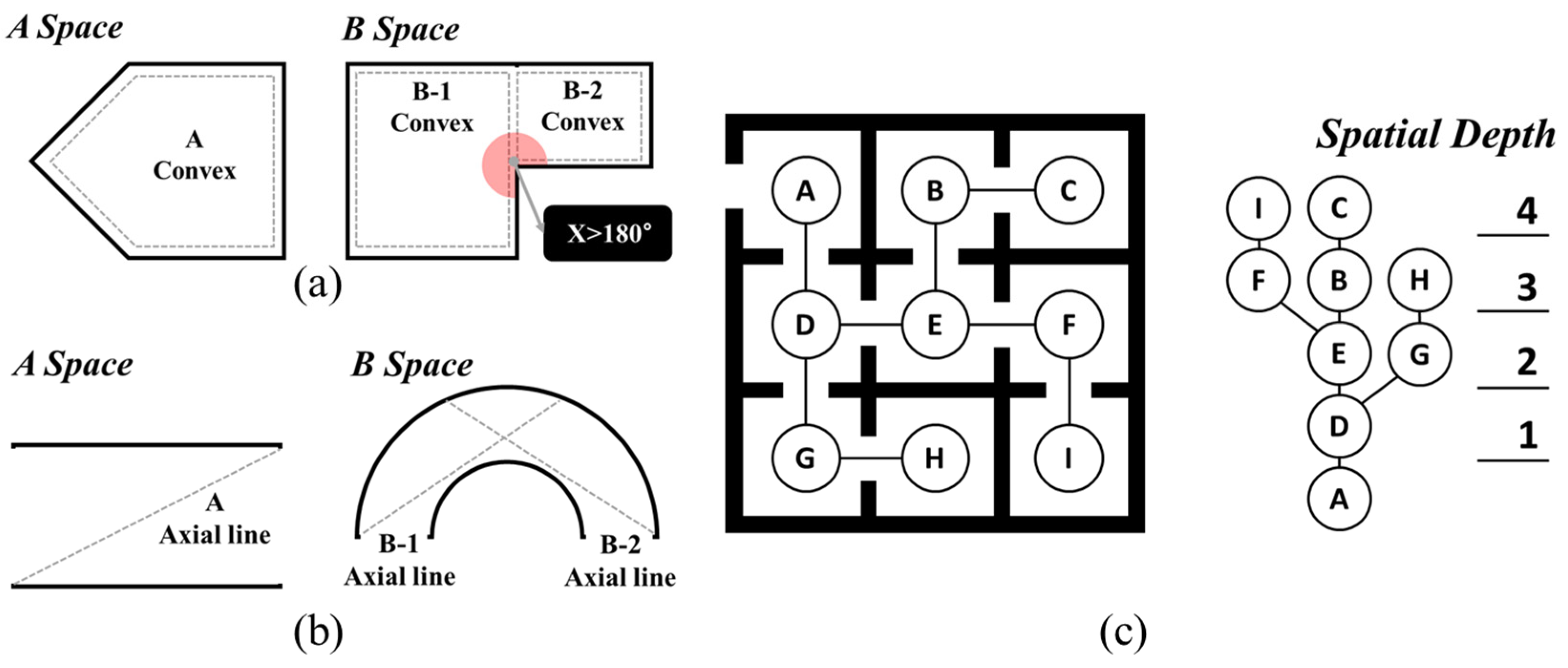
Space syntax [30] is a theoretical and analytical framework used to predict spatial usage patterns and quantify urban spatial hierarchy based on spatial depth. Developed by Hillier and Hanson at The Bartlett, University College London, this methodology defines spatial depth not as physical distance but as the number of spatial transitions required to move between locations [31]. Space syntax employs three primary spatial analysis forms: convex spaces, axial maps, and segment maps [30,32]. In architectural contexts, convex spaces analyze hierarchical spatial relationships [33,34,35]. In urban studies, axial and segment maps quantify spatial structures [36,37,38,39,40]. As illustrated in Figure 1a, in a convex space, the primary principle is to maintain the space as a closed polygon where all interior angles do not exceed 180°. If an interior angle exceeds 180°, analysis should be conducted by dividing the resulting concave space to obtain the smallest convex unit space. Axial lines should be established based on the visible connectivity observed within the space, and if it is refracted, one axial line should be divided into two or more axial lines to create a continuous connection. In addition, intersections between axial lines must reflect the connectivity of the spatial network (Figure 1b). Although convex space and axial maps are constructed differently, both ultimately rely on a topological structure that reflects spatial connectivity. As shown in Figure 1c, J-Graphs perform spatial analysis by designating a specific space as the root and visualizing the connectivity from that point to other spaces in a hierarchical structure.

Axial maps analyze urban accessibility and traffic by connecting spaces through optimal straight-line paths, considering visual continuity. Segment analysis is a network analysis method that incorporates weighted distances and angles to segment road networks based on axial maps [32]. Hence, if an axial map graphically represents urban spatial hierarchy based on physical structures, segment maps reflect actual human movement patterns along roads influenced by this spatial hierarchy. Figure 2 illustrates the difference between these two analysis methods.

Two primary space syntax indicators, control and integration, quantify spatial hierarchy. Control measures space’s influence over neighboring spaces, while integration is a measure of the accessibility of a space [30]. Integration is classified into global (i.e., accessibility within all spatial depths from a specific space to the entire area) and local integration (i.e., the accessibility and density of use of a within up to three adjacent spatial depths). Additionally, intelligibility can be quantified using the R² correlation coefficient, which is calculated as the correlation between global and local integration. A value closer to 1 denotes that the space is more systematic and recognizable.

Space syntax has been widely applied to analyze urban phenomena, including movement patterns, commercial revitalization, walkability, and crime distribution [31,36,37,38,39,40]. This study applies space syntax to evaluate Busan’s urban spatial hierarchy using key indicators: global integration, local integration, control, and intelligibility. Additionally, control and global integration are set as independent variables to empirically analyze the relationship between urban spatial hierarchy. Crime rate serves as the dependent variable. Given the study’s focus on urban spatial hierarchy and crime rate rather than human mobility patterns, we used axial maps.

Figure 3 and Equation (1) illustrate the methods for calculating the control and integration.

Table 2. An interpretation of the space syntax expressions.

Type	Interpretation
MD	Average spatial depth
TSDi	Total spatial depth in space i
S	The number of steps taken through space i
m	Number of steps from space i to the deepest space
K	The total number of spaces
Ks	Number of spaces in Step S
Dn	Correction factor
d(i, k)	Depth from space i to space k
n	Total number of nodes

summarizes the interpretation of space syntax expressions. Additionally, we used the depth map [41] program developed based on the space syntax to analyze the urban spatial hierarchy.

Table 3. Interpretation of key space syntax indicators.

Indicator		Definition	Significance
Integration	Global Integration	A measure of how central a space is within the overall urban network, based on the average shortest distance (depth) between all spaces (nodes) in the network.	Higher values indicate that the space is more easily accessible from across the city and is more centralized.
	Local Integration	An indicator that measures the connectivity of a given space to other spaces within a certain depth, reflecting local mobility.	This indicator typically analyzes network centrality within a region by measuring the degree of integration within three depths.
Control		A measure of how much influence a given space (axial line) has over the spaces it is connected to.	The more transitory a space is within the spatial structure, the higher the control.
Intelligibility		A measure of the correlation between local integration and global integration.	This indicator intuitively denotes how easy it is to understand the spatial structure.

presents an interpretation of the key indicators applied in this study.

$$I_{\left(i\right)}={\displaystyle \frac{D_n}{\frac{2}{n-2}(\frac{\sum _{k=1}^{n}d\left(i,k\right)}{n-1}-1)}}$$

(1)

2.2. Research Methods

This study defines the crime rate in Busan as the frequency of crimes per unit area and employs space syntax to examine its correlation with the urban spatial hierarchy. The research process consists of crime and spatial data collection, data processing and conversion, and statistical analysis. Figure 4 outlines the study’s methodology.

First, the crime frequency data were obtained from the 2023 crime occurrence dataset provided by the Ministry of the Interior and Safety’s Public Safety Map [42]. This dataset includes crime occurrences with specific temporal and spatial details. The study focuses on five major crimes: robbery, sexual assault, violence, larceny, and murder. We collected spatial data to construct a baseline road network using road centerline data from V-World, a platform managed by the Ministry of Land, Infrastructure, and Transport [43] (

Table 4. Sources of relevant data.

Data		Agency	Site Map	Website URL
Basic data (Urban spatial data and spatial crime data of Busan)	Road centerlines	Ministry of Land, Infrastructure and Transport	V-World	https://www.ngii.go.kr/kor/content.do?sq=237 (accessed on 30 December 2023)
	Crime hotspots	Ministry of the Interior and Safety	Public Safety Map	https://www.safemap.go.kr/main/smap.do?flag=2#majorCont02 (accessed on 30 December 2023)

).

Second, the road centerline data of Busan were projected using the Korea 2000 Korea Central Belt 2010 coordinate system in ArcGIS (ArcMap 10.2). Overpasses, tunnels, and rail transport codes were removed from the attribute data filter before extracting the data as a DXF file. We created an axial map in AutoCAD (v2024) based on these road centerlines. While creating axial lines, we divided the 10-level crime hotspot legends on the Public Safety Map into five layers (layer 1: levels 1–2; layer 2: levels 3–4; layer 3: levels 5–6; layer 4: levels 7–8; and layer 5: levels 9–10). We created layers in AutoCAD according to these crime hotspot levels, and corresponding axial lines were generated for each layer. Additionally, we defined crime-free areas as level 0 to differentiate them from crime-prone layers. We then designed axial lines to follow the principles of optimal spatial straight-line paths. However, to ensure data consistency, if an axial line intersected a crime hotspot, the line was adjusted to secure the intersection and assigned to the corresponding crime hotspot layer (Figure 5).

Third, after constructing the axial map of Busan’s urban space, we examined axial line intersections. The complete axial map (including all layers) was exported as a DXF file and imported into the depth map, which served as the primary dataset for analyzing Busan’s urban spatial hierarchy. We then extracted the analysis results in CSV format and prepared them as linked data for ArcGIS. Subsequently, each axial map layer (0–5) was then processed separately in AutoCAD and converted into DXF files. Layers were then imported into the depth map to generate the corresponding CSV files. Each layer’s axial line was imported into the depth map to obtain the XY coordinate system data of each layer’s axial line, not to produce the urban spatial hierarchy. Additionally, to incorporate the crime frequency (the dependent variable) into the attribute data when using the “XY to Line” function in ArcGIS, we created CSV files for layers 0–5, with a “dependent variable” item added after the X1, Y1, X2, and Y2 items to numerically indicate and enter the corresponding crime hotspot levels. Finally, we merged the six CSV files (layers 0–5) into one data frame.

Fourth, we imported the merged data frame into ArcGIS, where the “XY to Line” function reconstructed spatial data. During this process, we verified the accuracy of the “dependent variable” items in the attribute data filter. We then linked the reproduced data with the urban spatial hierarchy analysis results and data based on the X1 item, and the final dataset was derived. Data based on X1 were linked for two reasons. First, the sort order of the “Ref” in the data derived from the depth map did not align with the “FID” values in ArcGIS attribute data. Second, when creating the axial map, we adjusted the starting and ending points of the axial lines to prevent overlapping with other axial lines, ensuring that X1 remained unique within the dataset.

Fifth, we retained the dependent (layers 0–5) and independent variables (control and global integration) in the final dataset, while we deleted the other data. The remaining data were then imported into Statistical Product and Service Solutions version 25 to check for the normality, relative independence, and correlation of the sample. We then performed regression analysis to determine the statistical significance of control and global integrations on crime rates.

3. Results

3.1. Urban Spatial Hierarchy Analysis in Busan

The spatial analysis of Busan revealed substantial variation in its hierarchical connectivity and control. The control values ranged from 0.026 to 25.219, with an average of 1.000 (

Table 5. Urban spatial hierarchy of Busan.

Type	Integration		Control	Intelligibility
	Global	Local
Max	0.256	3.998	25.219	0.085
Min	0.089	0.333	0.026
Avg	0.182	1.378	1.000
Axial line	85,948 (crime-free area: 57,916; crime-prone area: 28,032)

and Figure 6). The global integration values, which reflect spatial accessibility, varied between 0.089 and 0.256, averaging 0.182. For local integration, the maximum, minimum, and average values were 3.998, 0.333, and 1.378, respectively. The intelligibility of Busan’s spatial structure, measured as the correlation between global and local integration, was 0.085, indicating a weak relationship. This suggests an asymmetrical urban spatial structure, highlighting the complexity of Busan’s spatial hierarchy. This study identified 85,948 axial lines, with approximately 32.62% classified as crime-prone areas or hotspots.

Spatial structure varied across Busan’s administrative districts, influencing crime occurrence patterns (

Table 6. Crime-prone areas by administrative district in Busan.

District (Abbreviated)	Area (km2)	Population Density	Areas Corresponding to Crime-Prone Areas (Number/Ratio of Axial Lines)
			Layer 1	Layer 2	Layer 3	Layer 4	Layer 5
Gangseo-gu (GS)	181.49	784.60/km2	887/80.42%	177/16.05%	35/3.17%	4/0.36%	0/0.00%
Geumjeong-gu (GJ)	65.28	3302.54/km2	800/42.44%	761/40.37%	260/13.79%	61/3.24%	3/0.16%
Gijang-gun (GIJ)	218.30	818.73/km2	1616/73.09%	413/18.68%	141/6.38%	39/1.76%	2/0.09%
Nam-gu (NG)	26.82	9477.44/km2	1132/62.40%	510/28.12%	135/7.44%	31/1.71%	6/0.33%
Dong-gu (DG)	9.87	8894.83/km2	1119/70.56%	352/22.19%	84/5.30%	24/1.51%	7/0.44%
Dongrae-gu (DR)	16.63	16,284.73/km2	1134/51.55%	692/31.45%	337/15.32%	27/1.23%	10/0.45%
Busanjin-gu (BSJ)	29.67	12,116.89/km2	1866/81.40%	324/14.14%	77/3.36%	18/0.79%	7/0.31%
Buk-gu (BG)	39.37	6949.35/km2	1166/65.10%	462/25.79%	126/7.04%	27/1.51%	10/0.56%
Sasang-gu (SS)	36.10	5621.39/km2	1607/70.82%	502/22.12%	113/4.99%	36/1.59%	11/0.48%
Saha-gu (SH)	41.77	7130.26/km2	1305/65.25%	502/25.10%	148/7.40%	40/2.00%	5/0.25%
Seo-gu (SG)	13.95	7461.58/km2	790/67.87%	279/23.97%	63/5.41%	26/2.23%	6/0.52%
Suyeong-gu (SY)	10.21	17,092.85/km2	1067/57.03%	591/31.59%	168/8.98%	41/2.19%	4/0.21%
Yeonje-gu (YJ)	12.10	17,005.45/km2	962/65.94%	391/26.80%	87/5.95%	16/1.10%	3/0.21%
Yeongdo-gu (YD)	14.20	7503.38/km2	1130/70.14%	353/21.91%	101/6.27%	24/1.49%	3/0.19%
Jung-gu (JG)	2.83	13,646.29/km2	383/76.29%	98/19.52%	18/3.59%	2/0.40%	1/0.20%
Haeundae-gu (HUD)	51.54	7381.61/km2	884/38.87%	941/41.39%	366/16.09%	79/3.47%	4/0.18%

). The largest administrative districts according to size and population density were Gangseo-gu (GS, 181.49 km²), Gijang-gun (GIJ, 218.30 km²), and Geumjeong-gu (GJ, 51.54 km²), while the smallest district was Jung-gu (JG, 2.83 km²). Additionally, the population density was highest in the order of Suyeong-gu (SY, 17,092 people/km²), Yeonje-gu (YJ, 17,005 people/km²), and Dongrae-gu (DR, 16,284 people/km²). Notably, in most administrative districts except GJ, DR, SY, and Haeundae-gu (HUD), layers 1 and 2 crime-prone areas accounted for more than 90% of incidents. These hotspots became more concentrated toward the city center. The results indicate that crime frequency tended to increase in areas with high control and global integration. This suggests that the urban spatial hierarchy influences crime occurrence.

3.2. Normality and Independence Analysis

A P-P plot was used to assess the normality of crime frequency, control, and global integration data. Figure 7 shows that residuals are distributed above and below the Y = 0 baseline, with most falling within ±0.04. The data aligned within the diagonal range of a normal P-P plot, indicating approximated normal distribution.

To evaluate relative independence, a Friedman test was conducted.

Table 7. Descriptive statistics and the Friedman test.

Category	N	Mean	Mean Rank	Std. Deviation	Minimum	Maximum	df	Chi-Square	Asymp. Sig.
Crime frequency	85,948	0.480	1.54	0.815	0	5	2	71,803.77	0.000
Control		1.002	2.74	0.698	0.333	25.219
Global integration		0.182	1.72	0.033	0.089	0.256

presents the mean ranks for crime frequency (1.54), control (2.74), and global integration (1.72), with df = 2 and χ² = 71,803.77. The p-values for all variables were significant at p < 0.001, confirming the relative independence of the dataset.

3.3. Correlation and Regression Analysis

After confirming normality and independence, correlations among crime frequency, control, and global integration were examined (

Table 8. Correlation analysis of variables.

Correlations		Crime Frequency	Control	Global Integration
Pearson Correlation	Crime frequency	1
	Control	0.129 **	1
	Global integration	0.095 **	0.024 **	1

** The correlation was significant at the 0.01 level (2-tailed).

). Pearson correlation coefficients between crime frequency and the independent variables (control and global integration) were 0.129 and 0.095, respectively, both significant at p < 0.01. These results indicate a weak positive correlation between crime frequency and urban spatial hierarchy indicators. These results suggest that the relationship between crime frequency and urban spatial hierarchy may be nonlinear rather than linear. Specifically, crime frequency may have a positive correlation with urban spatial hierarchy indicators at certain levels, but this correlation may change direction when specific thresholds are exceeded or influenced by other factors. The significance of this correlation indicates that urban spatial hierarchy is one of the factors affecting crime frequency. However, there are limitations in considering it as the sole determinant of crime occurrence.

Table 9. Model summary ^b.

Model	R	R Square	Adjusted R Square	Std. Error of the Estimate	Sig. F Change
1	0.158 a	0.025	0.025	0.805	0.000

^a Predictors: constant, control, and global integration; ^b dependent variable: crime frequency.

summarizes the regression model, with an R-value of 0.158, indicating a weak positive correlation between the dependent and independent variables. Control and global integration explained 2.5% of the crime frequency variation, with a standard error of 0.805. The ANOVA results (

Table 10. ANOVA ^a.

Model		Sum of the Squares	df	Mean Square	F	Sig.
1	Regression	1431.486	2	715.743	1105.868	0.000 b
	Residual	55,625.580	85,945	0.647
	Total	57,057.067	85,947

^a Dependent variable: crime frequency; ^b predictors: constant, control, global integration.

) show a regression sum of squares of 1431.486, an F-value of 1105.868, and a p-value < 0.001, confirming the statistical significance of the model. As outlined in

Table 11. Coefficients ^a.

Model		Unstandardized Coefficients		Standardized Coefficients	t	Sig.
		B	Std. Error	Beta
1	Constant	−0.072	0.016		−4.585	0.000
	Control	0.148	0.004	0.127	37.654	0.000
	Global integration	2.240	0.082	0.092	27.247	0.000

^a Dependent variable: crime frequency.

, the regression line intercept was −0.072. The independent variables, control (β = 0.148, t = 37.654) and global integration (β = 2.240, t = 27.247), were both significant at p < 0.001 for crime frequency. These findings suggest that the urban spatial hierarchy significantly influences crime frequency in Busan.

4. Discussion

This study employed space syntax analysis to examine Busan’s urban spatial structure and its relationship with crime frequency. The findings indicate that crime tends to be more frequent in areas with high control and global integration. This suggests that crime is more likely in structurally controlled and accessible spaces, aligning with theories that increased anonymity and potential victims contribute to crime. This contrasts with perspectives suggesting that enhanced spatial utilization improves natural surveillance and reduces crime.

In Busan, crime-prone areas were predominantly located near the city center. The low intelligibility of these areas reflects an asymmetrical and complex spatial structure, making navigation less intuitive. Notably, 32.62% of Busan’s axial lines were classified as crime hotspots, underscoring the significant association between urban space and crime. These findings emphasize the need for strategic urban planning to restructure urban space and improve public safety.

While it is evident that urban spatial hierarchy is one of the factors influencing crime frequency, it cannot be considered the sole determinant. These results are attributed to the nonlinear nature of the correlation and the low explanatory power of the independent variables in the regression model to fully explain the dependent variable. This study is significant as it establishes a causal relationship between crime frequency and urban spatial hierarchy in Busan. However, it also underscores the limitations of attributing crime frequency to a single factor and emphasizes the need for a comprehensive analysis that considers interactions with social and physical environmental factors, as noted in prior research. Therefore, it is crucial to first evaluate the relative influence of spatial, social, and physical factors within a given city to more accurately predict and explain crime occurrence. Furthermore, this study suggests the need for an in-depth understanding of how urban spatial restructuring affects crime occurrence. Notably, crime rates in Busan were concentrated near the city center, which indirectly suggests that the relationship between urban spatial structure and crime frequency is closely tied to spatial hierarchical characteristics, as well as patterns involving space use and human movement routes.

Our results indicate that crime occurrence is correlated with the hierarchical nature of Busan’s urban space. This suggests that crime can be more effectively prevented through comprehensive design and urban restructuring rather than approaches that strictly focus on enhancing public safety. This illustrates the potential to reduce crime by improving urban planning and spatial structure while emphasizing the need to redesign the city’s urban space to strengthen its crime prevention capabilities.

5. Conclusions

This study utilized space syntax analysis to explore the relationship between urban spatial hierarchy and crime rates in Busan, empirically assessing the correlation between crime frequency and urban spatial structure. We present the following main findings.

First, crime was more concentrated near the city center. Busan’s low intelligibility indicates an asymmetrical and complex spatial structure. This suggests a potential link between these spatial characteristics and crime occurrence.

Second, crime hotspots correlated with areas of high control and global integration. In downtown Busan, crime patterns were indirectly related to space usage patterns and human movement routes.

Third, urban spatial hierarchy exhibited a weak positive correlation with crime frequency. This demonstrates that urban spatial hierarchy influences crime occurrence patterns. However, the independent variables in the regression model exhibited low explanatory power for the dependent variable. Therefore, various external factors likely contribute to crime occurrence alongside the urban spatial hierarchy.

The crime rate analyzed in this study focused solely on the frequency of crimes in urban space and may not fully capture temporal changes in crime occurrence, which may limit the applicability of the findings. Additionally, while this study demonstrated a causal relationship between spatial structure and crime frequency, it did not consider the mutual influence of social factors, urban spatial structure, and the physical environment on crime occurrence. Consequently, future studies should employ structural equation models (SEMs) to analyze the mutual influences among these factors and assess the relative importance of each one. This approach is expected to facilitate an examination of not only the direct influence of urban spatial structure on crime occurrence but also the indirect effects of social factors and the physical environment on crime, mediated through spatial characteristics.

References

- Supreme Prosecutor’s Office. Crime Analysis. Available online: https://www.spo.go.kr/site/spo/crimeAnalysis.do (accessed on 20 May 2023).
- More than One Murder Every Day…Top 5 Most Violent Crimes in Korea. Maeil Business Newspaper. Available online: https://www.mk.co.kr/news/society/10595564# (accessed on 23 May 2023).
- Global Peace Index, Institute for Economics and Peace. Available online: https://www.economicsandpeace.org/wp-content/uploads/2024/06/GPI-2024-web.pdf (accessed on 5 September 2024).
- Crime Statistics, National Police Agency. Available online: https://www.police.go.kr/user/bbs/BD_selectBbsList.do?q_bbsCode=1115&estnColumn2 (accessed on 1 October 2024).
- Zhao, F.S.; Kim, S.W. A study on the safety evaluation of children’s parks in cities based on crime prevention through environmental design: Focused on Yangcheon-gu and Dongdaemun-gu. J. Korean Soc. Des. Cult. 2022, 28, 421–434. [Google Scholar] [CrossRef]
- Hwang, J.A.; Kang, J.Y. Relationship between the spatial distribution of crime-prone areas and the characteristics of urban decline: Focusing on crime risk indicators using GIS-based spatial statistics. KIEAE J. 2021, 21, 87–94. [Google Scholar] [CrossRef]
- Lee, S.J. Correlation analysis between spatial centrality and crime using the Korea Safety Map. J. Archit. Inst. Korea Plann. Des. 2017, 33, 69–76. [Google Scholar] [CrossRef]
- Kwon, Y.H. Effects of spatial vulnerability awareness and the residential environment on crime safety. Korea Spatial. Plann. Rev. 2024, 123, 59–74. [Google Scholar]
- Lee, J.Y. An analysis of the importance of planning elements for the border space of apartment complexes using AHP from the CPTED perspective. J. Korean Int. Spat. Des. 2024, 19, 69–80. [Google Scholar]
- Jing, Y.X.; Yang, J.; Cho, J.H. Demand analysis of CPTED in coastal areas using KANO model. Des. Res. 2024, 9, 84–93. [Google Scholar] [CrossRef]
- Busan Regional Safety Index, Busan Ilbo. Available online: https://www.busan.com/view/busan/view.php?code=2024022118153322188 (accessed on 25 July 2024).
- Kim, H.Y.; Kim, J.S. Defining boundaries of urban centers and measuring the impact for diagnosing urban spatial structure. J. Korean Assoc. Geogr. Inf. Stud. 2024, 27, 52–66. [Google Scholar] [CrossRef]
- Yang, Y.Q.; Pyo, E.S.; Yoo, J.W. A study on the characteristics of the new deal revitalization plan for residential district support project in Busan Metropolitan City. J. Korean Hous. Assoc. 2022, 33, 51–63. [Google Scholar] [CrossRef]
- Seo, Y.J.; Choi, J.W.; Ha, M.H. Evaluation of the socioeconomic impacts of port development and operation: Focusing on the firms in the new Busan port neighborhood areas. Korea. Logist. Rev. 2024, 34, 1–10. [Google Scholar] [CrossRef]
- Choi, H.R.; Lee, H.S.; Doe, G.Y. A study on the soft infrastructure planning for waterfront in port city: Focusing on the waterfront of Busan south port. J. Navig. Port Res. 2024, 48, 482–492. [Google Scholar] [CrossRef]
- Je, C.H.; Woo, S.K. A study on the strategic characteristics of the urban regeneration action plan: Focusing on urban regeneration projects in Busan. J. Korea Urban Regener. Assoc. 2023, 9, 32–57. [Google Scholar] [CrossRef]
- Total Crimes per 1,000 Population, E-Regional Index. Available online: https://kosis.kr/visual/eRegionJipyo/themaJipyo/eRegionJipyoThemaJipyoView.do (accessed on 25 July 2024).
- Kim, S.M.; Choi, J.Y.; Kang, Y.O. Measurement and visualization of perceived fear of crime by street level using street view images and deep learning technology. Korean Cartogr. Assoc. 2024, 24, 71–84. [Google Scholar] [CrossRef]
- Oh, H.N.; Kang, S.J.; Lee, G.W. An analysis of crime status and influence factors of new town in capital region of Korea. J. Community Saf. Secur. Environ. Des. 2023, 14, 91–120. [Google Scholar] [CrossRef]
- Kang, H. Effect of the local community’s perception of urban regeneration and CPTED on safety life satisfaction. Korean Secur. J. 2022, 70, 267–292. [Google Scholar] [CrossRef]
- Choi, J.H.; Park, S.M.; Woo, S.C. Multilevel analysis of specific crime fear in Seoul administrative districts. Seoul Stud. 2020, 21, 1–19. [Google Scholar] [CrossRef]
- Kim, H.S.; Jung, H.J.; Lee, J.S. The impact of CPTED on fear of crime levels of residents in low-density neighborhoods: Focusing on Seoul human town projects. Korean Inst. Cult. Archit. 2020, 69, 165–176. Available online: https://www.auric.or.kr/User/Rdoc/DocRdoc.aspx?returnVal=RD_R&dn=393070 (accessed on 30 December 2024).
- Yang, J.S. A study on the lighting design for crime prevention through environmental design (CPTED) in the urban space. J. Korean Int. Spat. Des. 2019, 14, 225–237. [Google Scholar] [CrossRef]
- Jeffery, C.R. Crime Prevention Through Environmental Design; Sage Publications: Beverly Hills, CA, USA, 1971. [Google Scholar]
- Newman, O. Defensible Space: Crime Prevention Through Urban Design; Collier Books: New York, NY, USA, 1973. [Google Scholar]
- Lee, G.U.; Lee, K.H. A study on crime and environmental characteristics in residential areas: Comparison of net residential street and neighborhood complex street. J. Community Saf. Secur. Environ. Des. 2021, 12, 243–276. [Google Scholar] [CrossRef]
- Zhao, X.; Park, E.-S.; Kim, J.; Lee, S.-Y.; Lee, H. Basic analysis of physical determinants affecting the distribution density of senior citizen centers around small apartment complexes, Focusing on administrative districts in Busan. Buildings 2024, 14, 929. [Google Scholar] [CrossRef]
- Zhao, X.L.; Hong, K.S. Analysis on accessibility of tourist city museums based on according to through angle and limit distance: Focusing on Busan Metropolitan City. J. Archit. Inst. Korea 2022, 38, 169–180. [Google Scholar] [CrossRef]
- Jeong, D.; Kim, M.; Song, K.; Lee, J. Planning a green infrastructure network to integrate potential evacuation routes and the urban green space in a coastal city: The case study of Haeundae District, Busan, South Korea. Total Environ. 2021, 761, 143179. [Google Scholar] [CrossRef]
- Hillier, B.; Hanson, J. The Social Logic of Space; Cambridge University Press: Cambridge, UK, 1984. [Google Scholar]
- Hong, K.S. Influence of the Relation Between a Crime Incidence and Physical Environment on Apartment Houses by Multiplex Analysis. Ph. D. Thesis, Kookmin University, Seoul, Republic of Korea, 2014. [Google Scholar]
- Turner, A. From axial to road-center lines: A new representation for space syntax and a new model of route choice for transport network analysis. Environ. Plan. B Plan. Des. 2007, 34, 539–555. [Google Scholar] [CrossRef]
- Fernandes, P.A. Space Syntax with logic programming: An application to a modern estate. Urban Sci. 2023, 7, 78. [Google Scholar] [CrossRef]
- Arslan, H.D.; Ergener, H. Comparative analysis of shopping malls with different plans by using space syntax method. Ain Shams Eng. J. 2023, 14, 102063. [Google Scholar] [CrossRef]
- Dawes, M.J.; Ostwald, M.J.; Lee, J.H. Examining control, centrality and flexibility in Palladio’s villa plans using space syntax measurements. Front. Archit. Res. 2021, 10, 467–482. [Google Scholar] [CrossRef]
- Atakara, C.; Allahmoradi, M. Investigating the urban spatial growth by using space syntax and GIS—A case study of Famagusta City. ISPRS Int. J. Geo-Inf. 2021, 10, 638. [Google Scholar] [CrossRef]
- Wu, Y.; Liu, Q.; Hang, T.; Yang, Y.; Wang, Y.; Cao, L. Integrating restorative perception into urban street planning: A framework using street view images, deep learning, and space syntax. Cities 2024, 147, 104791. [Google Scholar] [CrossRef]
- Qanazi, S.; Hijazi, I.H.; Shahrour, I.; Meouche, R.E. Exploring urban service location suitability: Mapping social behavior dynamics with space syntax theory. Land 2024, 13, 609. [Google Scholar] [CrossRef]
- Karimi, K. The configurational structures of social spaces: Space syntax and urban morphology in the context of analytical, evidence-based design. Land 2023, 12, 2084. [Google Scholar] [CrossRef]
- Colding, J.; Samuelsson, K.; Marcus, L.; Gren, Å.; Legeby, A.; Berghauser Pont, M.; Barthel, S. Frontiers in social–Ecological urbanism. Land 2022, 11, 929. [Google Scholar] [CrossRef]
- Depth Map, UCL Space Syntax. Available online: https://www.spacesyntax.online/ (accessed on 30 December 2024).
- Ministry of the Interior and Safety. Public Safety Map. Available online: https://www.safemap.go.kr/main/smap.do?flag=2#majorCont02 (accessed on 30 December 2023).
- Ministry of the Interior and Safety. Busan City Spatial Data. Available online: https://www.ngii.go.kr/kor/content.do?sq=237 (accessed on 30 December 2023).
Figure 1.
Example of spatial analysis form: (a) convex space, (b) axial map, (c) spatial depth and J-graph.
Figure 2.
Difference between axial map and segment map: (a) axial map and (b) segment map.
Figure 3.
A calculation of the control.
Figure 4.
Research procedure.
Figure 5.
Axial map reflecting crime frequency in Haeundae district of Busan: (a) public safety map and (b) AutoCAD editing principles.
Figure 6.
Current status of Busan: (a) administrative districts, (b) crime-prone areas, (c) global integration graph, (d) local integration graph, (e) control graph.
Figure 7.
Normal and detrended normal P-P plot: (a) crime frequency, (b) control, (c) global integration.