Research on Energy Consumption, Thermal Comfort, Economy, and Carbon Emissions of Residential Buildings Based on Transformer+NSGA-III Multi-Objective Optimization Algorithm

Abstract

This study proposes a Transformer–NSGA-III multi-objective optimization framework for high-rise residential buildings in Haikou, a coastal city characterized by a hot summer and warm winter climate. The framework addresses four conflicting objectives: Annual Energy Demand (AED), Predicted Percentage of Dissatisfied (PPD), Global Cost (GC), and Life Cycle Carbon (LCC) emissions. A localized database of 11 design variables was constructed by incorporating envelope parameters and climate data from 79 surveyed buildings. A total of 5000 training samples were generated through EnergyPlus simulations, employing jEPlus and Latin Hypercube Sampling (LHS). A Transformer model was employed as a surrogate predictor, leveraging its self-attention mechanism to capture complex, long-range dependencies and achieving superior predictive accuracy (R² ≥ 0.998, MAPE ≤ 0.26%) over the benchmark CNN and MLP models. The NSGA-III algorithm subsequently conducted a global optimization of the four-objective space, with the Pareto-optimal solution identified using the TOPSIS multi-criteria decision-making method. The optimization resulted in significant reductions of 28.5% in the AED, 24.1% in the PPD, 20.6% in the GC, and 18.0% in the LCC compared to the base case. The synergistic control of the window solar heat gain coefficient and external sunshade length was identified as the central strategy for simultaneously reducing energy consumption, thermal discomfort, cost, and carbon emissions in this hot and humid climate. The TOPSIS-optimal solution (C = 0.647) effectively balanced low energy use, high thermal comfort, low cost, and low carbon emissions. By integrating the Energy Performance of Buildings Directive (EPBD) Global Cost methodology with Life Cycle Carbon accounting, this study provides a robust framework for dynamic economic–environmental trade-off analyses of ultra-low-energy buildings in humid regions. The work advances the synergy between the NSGA-III and Transformer models for high-dimensional building performance optimization.

1. Introduction

In recent decades, challenges such as resource depletion, high energy consumption, and environmental pollution have intensified owing to global population growth, accelerated urbanization, and rising societal demands [1]. The construction sector is a major contributor, accounting for over 30% of global energy consumption and carbon emissions, which leads to significant environmental strain and resource wastage [2]. Consequently, governments and researchers worldwide are advocating for the industry’s transition towards energy conservation, emissions reduction, and sustainable development [3]. In line with this, China has actively promoted the greening of its building stock, with the extensive implementation of Passive House (PH) technology. Originating in Germany, the PH standard achieves ultra-low energy consumption primarily through optimized building envelope design, thereby minimizing reliance on active mechanical systems [4]. Studies have demonstrated that PH buildings can reduce heating and cooling energy demand by 80–90% compared to conventional structures, representing a substantial energy-savings potential. This positions PH as a critical pathway for decarbonizing the building sector [5].

The pursuit of passive building design, despite its significant energy-saving and comfort advantages, necessitates balancing multiple conflicting objectives—namely, energy consumption, thermal comfort, economic cost, and carbon emissions. This complexity has driven the advancement of multi-objective optimization (MTO) research. Early studies primarily addressed single-objective energy optimization, employing tools like EnergyPlus for simulation and machine learning techniques, such as support vector machines and neural networks, to enhance predictive accuracy [6]. Subsequent research has evolved to integrate machine learning with meta-heuristic algorithms. For instance, Hosseini et al. [7] combined a Genetic Algorithm (GA) and Particle Swarm Optimization (PSO) to refine a Deep Neural Network (DNN) architecture for energy prediction. Gupta et al. [8] developed a Deep Reinforcement Learning (DRL)-based heating controller to improve thermal comfort. Lin et al. [9] proposed a three-stage framework integrating Latin Hypercube Sampling with a Genetic Algorithm, following the paradigm of “Parametric Design—Machine Learning Agent Model—Population Intelligence Optimisation.” Jafari and Valentin [10] optimized the life cycle cost for a residential building in the southern US climate, providing optimal retrofit solutions and associated investment costs to demonstrate the financial viability for homeowners.

Early MTO research in building design primarily addressed bi-objective conflicts. Negendahl and Nielsen [11] pioneered a framework that explicitly modeled buildings’ energy consumption and capital costs as conflicting objectives. Wang et al. [12] employed EnergyPlus simulations combined with Gradient Boosting Decision Trees (GBDTs) and NSGA-II to optimize energy consumption and thermal comfort for residential buildings in China’s cold regions. Similarly, Luo et al. [13] utilized Grasshopper, with its plugins, and the HypE algorithm for the MTO of life cycle energy consumption and life cycle cost of cold region office buildings. Xu et al. [14] applied EnergyPlus, artificial neural networks, and NSGA-II for the multi-objective optimization of thermal comfort and daylighting performance in a public building in Nanjing. Chen et al. [15] optimized the energy consumption and thermal comfort of a teaching building in Wuhan, validating their framework using a hybrid LSSVM-NSGA-II method. Gou et al. [16] conducted an MTO of energy consumption and thermal comfort for a Shanghai residential building, demonstrating significant potential for improving both comfort and energy savings.

Al-Mindeel et al. [17] reviewed the MTO literature from 2010 to 2023, noting that most studies prior to 2015 addressed only a bi-objective optimization for energy and thermal comfort. Subsequently, tri-objective optimization emerged as a research focus. Alimohamadi and Jahangir [18] proposed a MATLAB(R2024a)–EnergyPlus co-simulation framework for the tri-objective optimization of energy consumption, the PMV index, and retrofit cost. Wu et al. [19] developed a framework combining Bayesian optimization with an Extreme Gradient Boosting Tree (BO-XGBoost) and NSGA-II, achieving significant improvements over the baseline: a 44.1% reduction in energy use, a 10.9% reduction in thermal discomfort, and a 1.7% improvement in daylighting. Benaddi et al. [20] integrated TRNSYS simulations with GenOpt to implement an MTO for optimal envelope design, considering the life cycle cost, Life Cycle Carbon emissions, and thermal discomfort time.

With the advancement of global carbon neutrality goals, carbon emissions have become a critical fourth dimension in building performance optimization. Canbolat et al. [21] applied NSGA-II for an MTO targeting minimal cost and CO₂ emissions. Chen et al. [22] investigated Life Cycle Carbon emissions, life cycle cost, and indoor discomfort hours for an office building in Qingdao using an integrated learning model with optimization algorithms, thereby demonstrating the feasibility of their framework. Kang et al. [23] developed a data-driven methodology integrating PSO, support vector machines (SVMs), and NSGA-III to optimize carbon emissions, economic cost, and thermal comfort, demonstrating enhanced building performance.

The Non-dominated Sorting Genetic Algorithm II (NSGA-II) has become a mainstream choice for building MTOs due to its efficient non-dominated sorting and crowding distance mechanisms for diversity preservation [24]. Developed by Deb et al. in 2002 [25], NSGA-II established a performance benchmark in the field. Commonly used MTO algorithms include the Vector Evaluated Genetic Algorithm (VEGA) [26], the Multi-Objective Genetic Algorithm (MOGA) [27], the Niched Pareto Genetic Algorithm (NPGA) [28], the Non-dominated Sorting Genetic Algorithm (NSGA) [29], the Fast Non-dominated Sorting Genetic Algorithm-II (NSGA-II) [25], the Non-dominated Sorting Genetic Algorithm-III (NSGA-III) [30], the Strength Pareto Evolutionary Algorithm (SPEA) [31], and the Strength Pareto Evolutionary Algorithm-II (SPEA-II) [32]. A comparative analysis of the core principles and relative advantages of these eight algorithms is provided in

Table 1. Comparative analysis of multi-objective optimization algorithms.

Multi-Objective Optimization Algorithm	Proposer and Time of Proposal	Basic Idea	Advantages	Disadvantages
VEGA	Schaffer, 1985 [26]	Equal molecular populations, proportional selection, crossover, and variation.	The selection mechanism is simple. Easy to implement.	It is difficult to determine a unified fitness function. Some outstanding parent individuals may be lost.
MOGA	Fonseca & Fleming, 1993 [27]	Based on non-inferior ranking, linear interpolation fitness assignment, selection, crossover, and mutation.	The algorithm is simple and easy to operate, with high execution efficiency.	Overly relies on the selection of shared parameters. Excessive local pressure is prone to premature convergence.
NPGA	Horn & Nafplioti, 1993 [28]	Tournament selection based on Pareto dominance, fitness sharing, crossover, and mutation.	Quickly finds the non-inferior solutions. The computational complexity does not depend on the number of targets.	Shared parameters need to be set. The tournament mechanism needs to be selected. Low search efficiency.
NSGA	Srinivas & Deb, 1994 [29]	Based on non-inferior ranking, virtual fitness assignment, tournament selection, crossover, and mutation.	There is no limit to the number of optimization targets. The non-inferior solutions are uniformly distributed. Multiple equivalent solutions coexist.	Shared parameters need to be set. High computational complexity. Some excellent parent individuals may be lost.
NSGA-II	Deb & Pratap, 2002 [25]	Based on fast non-dominated sorting, congestion calculation, elite retention, tournament selection, crossover, and mutation.	High execution efficiency, easy to implement, and strong global search ability.	Poor local search ability. Some optimal solutions are lost.
NSGA-III	Jain et al., 2014 [30]	Reference points, non-dominated sorting, and many objectives.	High dimensional, uniform distribution, and efficiency.	Complexity, parameter sensitivity, and limited scenarios.
SPEA	Zitzler & Thiele, 1999 [31]	Based on Pareto sorting, elite retention, fitness assignment, tournament selection, crossover, and mutation.	Non-inferior solutions are uniformly distributed.	High computational complexity. The boundary solution may be lost.
SPEA-II	Zitzler & Thiele, 2001 [32]	Based on Pareto sorting, external archiving, elite retention, fitness assignment, tournament selection, crossover, and mutation.	Elite retention and cluster analysis to maintain population diversity. The solution set is uniformly distributed.	Cluster analysis and calculation take a relatively long time.

.

Multi-objective optimization (MTO) algorithms are extensively applied across various engineering disciplines [33]. In the building performance domain, comparative studies have established the efficacy of specific algorithms. For instance, Rafati et al. [34] compared NSGA-II and SPEA-2 for optimizing energy and visual comfort, demonstrating NSGA-II’s superior performance. Similarly, Cheraghi and Jahangir [35] found that NSGA-II outperformed MOPSO for optimizing a building’s hybrid energy system, offering broader solution coverage and more uniform dispersion along the Pareto front. NSGA-II has been consistently noted for its superior convergence to the true Pareto frontier, with diverse and uniformly distributed solutions compared to alternative algorithms [24]. This effectiveness has been further evidenced by studies such as that of Baghoolizadeh et al. [36], who applied NSGA-II to jEPlus outputs to achieve a 40–50% reduction in annual building energy consumption while simultaneously improving the visual comfort by 70–100% and the thermal comfort by 10–40%. Peng et al. [37] integrated carbon emission factors into construction costs, deriving Pareto-optimal solutions via NSGA-II and employing the efficacy coefficient method for decision-making. The algorithm has proven particularly effective for solving nonlinear parametric regression and optimization problems with up to three objectives [38]. For higher-dimensional problems, NSGA-III was developed as a successor [39]. Jain et al. [30] systematically proposed NSGA-III for high-dimensional MTO (exceeding three objectives), demonstrating its capability for superior Pareto frontier distribution. Consequently, NSGA-III represents an advanced and widely adopted Genetic Algorithm for complex optimization tasks [40].

However, the existing algorithms often face dimensionality challenges and convergence issues when handling four or more conflicting objectives, such as energy consumption, thermal comfort, economy, and carbon emissions. This limitation necessitates the integration of novel predictive intelligence methods. The Transformer model, proposed by Vaswani et al. [41], introduced a powerful alternative to recurrent (RNN) and convolutional neural networks (CNNs) through its self-attention mechanism for sequence modeling. Its core advantages include parallel computing capability through multi-head attention, which captures multi-scale features efficiently, and enhanced long-term dependency modeling, which is critical for correlating complex, time-dependent variables, such as historical weather patterns, equipment states, and energy fluctuations. These properties have led to its adoption in building science; for example, Clemente et al. [42] applied a global Transformer architecture for multi-room temperature prediction, enabling single-model training across all rooms to optimize HVAC energy use. Spencer et al. [43] explored transfer learning with Transformers for energy consumption forecasting, and Xu et al. [44] developed an encoder–decoder architecture combining a deformable CNN and a query-based Transformer for multi-task learning.

A review of existing research indicates that studies on passive ultra-low-energy technology have predominantly focused on hot summer and cold winter regions. For instance, Huo et al. [45] employed a GA-ANN integration to optimize indoor comfort, energy consumption, and retrofit costs for an existing building in this climate. Xiang et al. [46] developed a probabilistic behavioral model for the multi-objective optimization of ultra-low-energy residences to advance developments in these regions. Qian et al. [47] analyzed building wind environments and envelope thermal performance via a simulation, proposing passive design methods for medium-small gymnasiums. In contrast, the research on high-rise residential buildings in hot summer and warm winter coastal areas remains notably limited.

Addressing this research gap, this study investigates the MTO of high-rise residential buildings in Haikou, which features a tropical oceanic monsoon climate characterized by prolonged summers, high temperatures, humidity, and intense solar radiation. The primary innovation of this work is the novel integration of a Transformer surrogate model with the NSGA-III algorithm to create a robust framework for the synergistic optimization of four key objectives: energy consumption (AED), thermal comfort (PPD), Global Cost (GC), and Life Cycle Carbon (LCC) emissions. A comparative analysis demonstrates the Transformer’s superior predictive accuracy over mainstream alternatives like CNN and MLP models, while NSGA-III enables effective global optimization of this high-dimensional objective space. This integrated approach successfully identifies the Pareto-optimal frontier for building optimization in hot summer, warm winter coastal regions, thereby providing actionable insights into optimal envelope configurations and passive technology strategies tailored for tropical coastal environments.

Based on the preceding literature review and building upon the foundational work of previous researchers, this study presents the following key innovations relative to existing studies:

• The development of a comprehensive four-dimensional optimization framework targeting energy consumption, thermal comfort, economic cost, and carbon emissions, specifically tailored for the challenges of high-temperature, high-humidity, and high-solar radiation climates. This framework successfully identifies the Pareto-optimal frontier for high-rise residential buildings in hot summer, warm winter coastal regions, enabling synergistic optimization of these critical objectives.
• The establishment of a localized and empirically derived database comprising 11 key design parameters. These parameters were extracted from an analysis of typical wall, window, and roof structures of high-rise residences in Haikou, ensuring the generation of region-specific and representative design solutions.
• The integration of EPBD Global Cost methodology with a whole Life Cycle Carbon-accounting approach. This integration facilitates a dynamic economic–environmental trade-off analysis during the optimization process, thereby advancing the assessment standards for ultra-low-energy buildings in humid climates.
• The implementation of a Transformer model as a high-accuracy surrogate predictor, achieving R² values ≥ 0.998 when trained on localized data. This novel application is coupled with the NSGA-III algorithm for effective four-objective optimization, followed by a TOPSIS-based method for selecting the final solution from the Pareto frontier, establishing a robust methodology for high-dimensional building performance problems.

2. Methodology and Settings

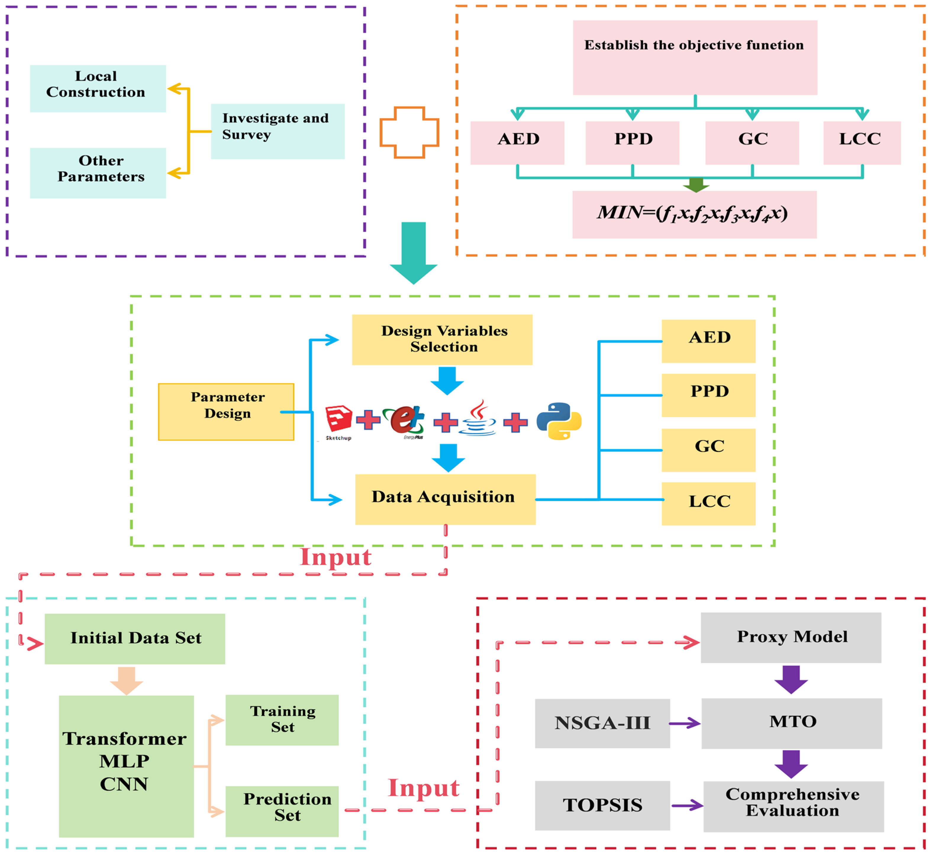
This study structures the optimization design for residential buildings in Haikou—addressing energy consumption, thermal comfort, economy, and carbon emissions—into three phases: (1) Methodology and Parameter Settings, (2) Results and Discussion, and (3) Conclusions. The first phase elaborates on the construction of the optimization model and the research methods applied at each stage, with the overall framework depicted in Figure 1.

2.1. Research Summary

To evaluate the current thermal performance of residential buildings in Haikou, a survey was conducted of 79 newly built commercial residential buildings constructed within the last 15 years. The key parameters, such as the floor area, standard floor layout, building orientation, and number of stories, were investigated. A summary of the results is presented in

Table 2. Statistics on residential buildings’ areas.

Number of Buildings	Standard Floor Building Area (m2)	Number of Buildings
7	≥1000	3
17	1000 > X ≥ 800	10
25	800 > X ≥ 600	21
22	600 > X ≥ 400	33
8	400 > X ≥ 0	12

and Figure 2.

The survey results indicate that high-rise buildings ranging from 15 to 25 stories dominate the residential building stock in the Haikou area, comprising nearly 50% of the sampled buildings. The majority of these structures (87.5%) adopt a north–south orientation, with the unit floor areas typically ranging from 80 to 160 m². In accordance with the latest national standard, the “Code for Residential Projects” issued by the Ministry of Housing and Urban–Rural Development, the floor-to-ceiling height of new residential buildings should not be less than 3 m.

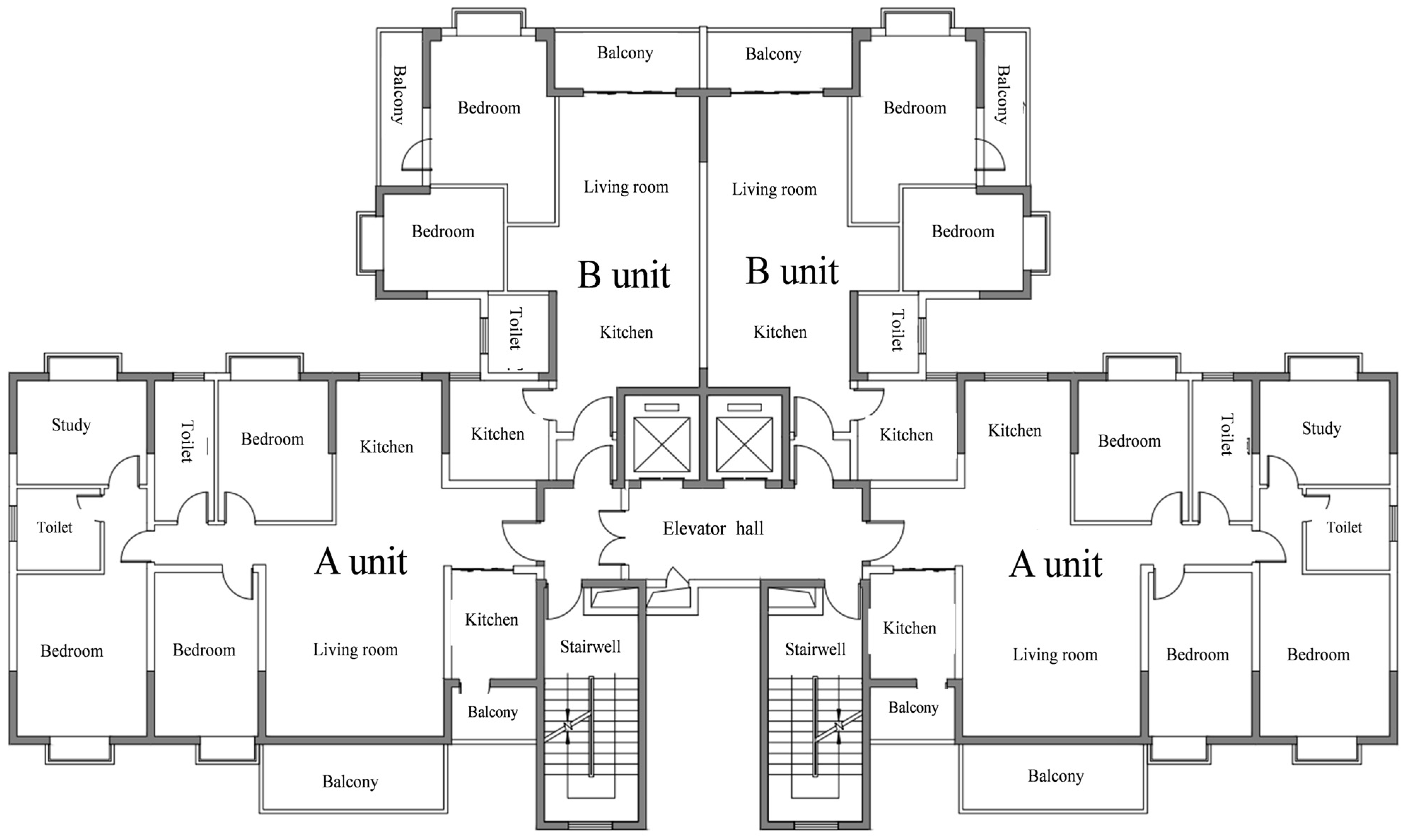
Analysis of the 79 residential buildings enabled the establishment of a standardized floor plan, as illustrated in Figure 3. The benchmark building’s standard floor configuration consists of two unit types: Type A, with a net floor area of 125.58 m², containing three bedrooms, a living room, and two bathrooms designed for five occupants; and Type B, with a net floor area of 85.16 m², featuring two bedrooms, a living room, and one bathroom designed for three occupants. Based on these standardized parameters, a representative 15-story commercial residential building with a point-tower layout was developed to accurately reflect the typical architectural characteristics and spatial configurations observed in the surveyed sample.

To improve the simulation accuracy, the building envelope configurations were informed by historical construction practices and regional engineering standards, specifically referencing the Central/Southern Region Engineering Construction Standards (2005, 2011, and 2015 editions).

Table 3. Construction of envelope structure.

Building Envelope	Construct Name	Thickness (mm)	U (W/m2·K)
Exterior wall	Aerated concrete wall	245	0.818
	Painted exterior wall (1)	242	1.03
	Painted exterior wall (2)	244	1.028
	Real stone painted exterior wall	244	1.007
Glass	Double-layer insulating glass	24	2.685
	Low-e insulating glass	21	2.33
	Low-e insulating glass (Argon)	21	1.94
	High-permeability, Low-e insulating glass	24	1.65
Roof	Inverted top roof (1)	233	0.806
	Inverted top roof (2)	264	0.732
	Inverted top roof (3)	202	0.679

summarizes the typical envelope assemblies identified for Haikou, comprising four external wall types, four fenestration systems, and three roof structures. The complete technical specifications for these components are provided in Appendix A.

The meteorological data for Haikou was obtained from the EnergyPlus official website and the EPW Map resource, guaranteeing the data’s regional specificity and accuracy for the study location. The analysis indicates consistently elevated dry-bulb and wet-bulb temperatures, with the summer (May to October) peaks notably reaching approximately 35 °C and 25 °C, respectively. The relative humidity averages approximately 90%, which is substantially higher than the standard comfort range of 40–60%. Wind speeds average between 3 and 5 m/s, with summer (June to September) peaks of up to 11 m/s, primarily due to monsoon influences. The infrared radiation exhibits seasonal fluctuations between 350 and 450 Wh/m², reaching its highest levels during the summer (May to September) and its lowest in the winter (November to February). These climatic characteristics confirm Haikou’s tropical monsoon climate, highlighting the necessity of optimizing building energy efficiency and occupant comfort.

2.2. Establishment of the Optimization Model

2.2.1. Establishment of Optimization Objectives

This study establishes four optimization objectives for high-rise residential buildings in Haikou, informed by the local climate, geography, and user needs: Annual Energy Demand (AED), Predicted Percentage Dissatisfied (PPD), Global Cost (GC), and Life Cycle Carbon (LCC). These metrics, respectively, represent energy consumption, thermal comfort, economic performance, and environmental impact. Critical trade-offs are identified between the AED and PPD and between the GC and LCC. In contrast to previous studies that have primarily focused on dual objectives—such as energy–cost or comfort–carbon—this research concurrently couples all four indicators. It advances a whole-life carbon analysis through the LCC metric and explicitly addresses the inherent conflict between the AED and PPD in hot–humid climates. Consequently, this work offers a superior multidimensional optimization framework for tropical buildings compared to conventional models. The detailed validation methodology and comprehensive boundary conditions are elaborated in Section 2.3.1, with the complete parameter sets provided in Appendix D.

(1)

Annual Energy Demand (AED)

Haikou’s climate, classified as a hot summer/warm winter zone (Zone B), is characterized by extended summers and the absence of a winter season, thereby eliminating the need for residential heating. EnergyPlus simulates the building’s performance by modeling the annual energy consumption for cooling (ACEC), lighting, and equipment. The energy use across all operational conditions is incorporated into the economic and carbon calculations. However, optimization is performed exclusively on the cooling energy during the defined cooling period (from 15 April to 15 November, totaling 214 days, Beijing time), as the demands for lighting and equipment remain constant during the optimization process [48]. The AED is specifically defined as the annual cooling energy consumption to isolate and evaluate the effect of envelope optimization on the most climate-sensitive energy end-use. Conversely, to ensure a comprehensive life cycle assessment, the GC and LCC calculations incorporate the total operational energy, including lighting and equipment. This inclusion is critical because these components represent actual, ongoing costs and emissions, thereby providing a more realistic evaluation of the building’s overall performance. The calculation is as follows:

$$AED=ACEC$$

(1)

$$ACEC={\displaystyle \frac{\sum _{i=1}^{i=n}E{C}_{hi}}{M}}$$

(2)

$$AEL={\displaystyle \frac{\sum _{i=1}^{i=j}E{C}_{hi}}{M}}$$

(3)

$$AEE={\displaystyle \frac{\sum _{i=1}^{i=k}E{C}_{hi}}{M}}$$

(4)

where n is the number of annual cooling hours; j is the number of annual lighting hours; k is the number of annual hours of use of electrical equipment; EC_hi is the hourly energy demand (kWh); and M is the floor area (m²).

(2)

Predicted Percentage of Dissatisfied (PPD)

In this study, thermal comfort is evaluated using the Predicted Percentage of Dissatisfied (PPD) index. The PPD is calculated based on Fanger’s Predicted Mean Vote (PMV) model, in accordance with the ISO 7730 standard [49], to estimate the percentage of occupants who are likely to feel thermally uncomfortable. The model is implemented using the following equation:

$$PPD=100-95\cdot \mathrm{e}\mathrm{x}\mathrm{p}\left(-0.03353\cdot PM{V}^4-0.2179\cdot PM{V}^2\right)$$

(5)

where the PMV (Predicted Mean Vote) is calculated through the heat balance equation, specifying parameters such as the metabolic rate (M), garment thermal resistance (Icl), air flow rate (Va), air temperature (Ta), and mean radiant temperature (Tr). This chain of formulas is implemented in the EnergyPlus source code through segmented iterations to ensure accurate modeling of radiative, convective, and evaporative heat exchanges. The area-weighted average of 120 setup air-conditioned rooms for the whole building is considered in the PPD setup of this paper.

(3)

Economic evaluation with reference to the Global Cost (GC) proposed by the EU Energy Performance of Buildings Directive (EPBD)

A PH represents a key development focus for future construction due to its ultra-low energy consumption. However, its higher construction costs in China necessitate economic analysis of envelope structures and associated energy use. This study adopts and adapts the EPBD Global Cost methodology [50], proposing an economic assessment framework integrated with building envelope systems. The computational framework for GC is expressed as follows:

$$GC=C_I+\sum _{i=1}^T\left[C_a\left(i\right)\right]$$

(6)

where C_I is the initial investment cost (different construction materials, construction, and installation costs) and Ca(i) is the annual cost in year i (energy costs for cooling, lighting, and electrical equipment).

This study employs the Global Cost methodology to evaluate envelope configurations. The initial investments for structural modifications and operational energy costs (cooling, lighting, and equipment) are calculated over a 50-year life cycle. All the cost parameters adhere to the Hainan Provincial Engineering and Construction standards, with detailed specifications provided in Appendix B.

(4)

Life Cycle Carbon (LCC)

Life Cycle Carbon emissions encompass five phases: material production, transportation, construction, demolition, and operational energy use. Calculations span a 50-year period, with detailed methodology provided in Appendix C.

2.2.2. Establishment of the Objective Function

Combining the above analysis, the AED, PPD, GC, and LCC are selected as the optimization objectives and are minimized in this paper, and the optimization function model is as follows:

$$Min=\left\{f_{1}x\right.,f_{2}x,\left.f_{3}x,f_{4}x\right\},x=\left[x_1,x_2,\dots ,x_n\right]$$

(7)

where f₁ is AED, f₂ is PPD, f₃ is GC, and f₄ is LCC.

2.2.3. Establishment of MTO Path

Multi-objective optimization (MTO) resolves conflicting objectives by formulating mathematical models that minimize the target functions under specified constraints to identify optimal solutions [51]. Building optimization frequently involves inherent trade-offs, where the enhancement of one objective may compromise others. To address this challenge, a three-step framework was established for high-rise residential buildings in Haikou: (1) a comparison and optimization of predictive algorithms, (2) an NSGA-III-based MTO search, and (3) a comprehensive evaluation using the TOPSIS method.

(1)

Predictive Modeling

Direct coupling of EnergyPlus and NSGA-III is computationally prohibitive for the multi-objective optimization of passive ultra-low-energy buildings. A single simulation can require tens of minutes to hours, whereas NSGA-III typically necessitates thousands of evaluations. To overcome this limitation, a Transformer model was implemented as a data-driven surrogate to establish nonlinear mappings between the inputs—the envelope characteristics and equipment parameters—and the outputs (AED, PPD, LCC, and GC). The Transformer model uniquely achieved sub-second predictive inference with exceptional accuracy (R² ≥ 0.998), outperforming both the CNN and MLP models at capturing the high-dimensional parameter interactions, thereby enabling efficient NSGA-III optimization.

The encoder–decoder architecture of the Transformer provides distinct advantages for this application. Its multi-head attention mechanism effectively captures global dependencies within sequences of building parameters, while its layer normalization ensures training stability. These features facilitate superior modeling of the complex, nonlinear interactions between energy, comfort, economy, and carbon metrics [41]. The combination of sub-second inference speed and ultra-high accuracy (R² ≥ 0.998) renders the Transformer uniquely suited for high-dimensional MTO, a domain where traditional models often fail to balance computational speed with predictive precision.

Convolutional neural networks (CNNs) originated with LeNet-5, which pioneered the integration of convolutional, pooling, and fully connected layers for handwritten digit recognition [52]. While the core mechanisms—such as local receptive fields, weight sharing, and hierarchical feature abstraction—established CNNs as cornerstones of computer vision, they exhibit limitations for capturing long-range dependencies and adapting to dynamic, non-Euclidean relationships. These shortcomings are critical in the context of building performance simulation, where the parameters exhibit complex, global interactions [53].

A Multilayer Perceptron (MLP) employs fully connected layers with nonlinear activation functions, trained via backpropagation. This architecture maintains strong universal function approximation capabilities through its architectural simplicity, serving as a fundamental baseline for benchmarking neural network performance.

(2)

NSGA-Ⅲ MTO

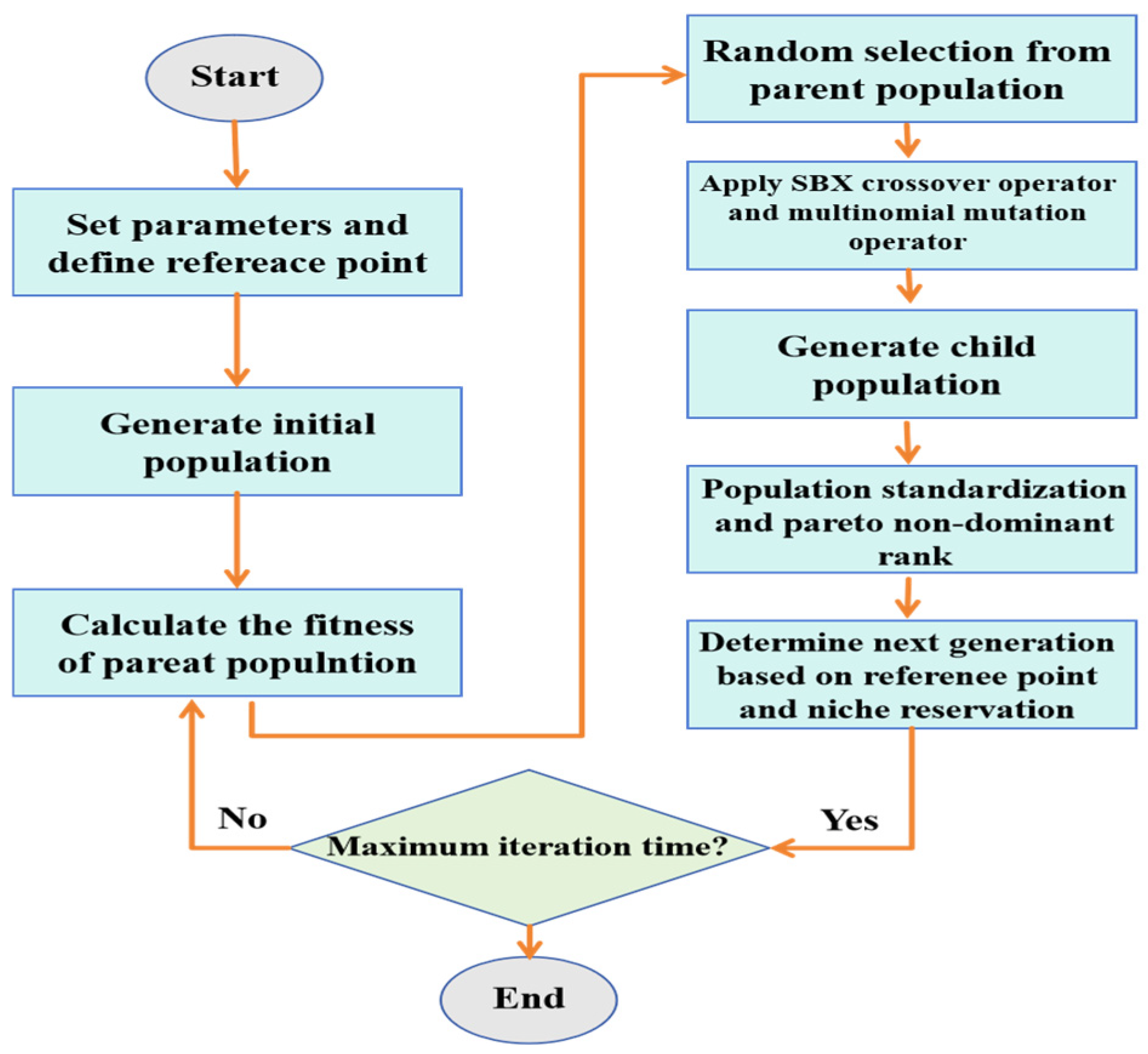
NSGA-III, an extension of NSGA-II, is a third-generation multi-objective optimization algorithm that introduces a reference point mechanism to address the challenges of high-dimensional spaces [39]. The framework retains the core components of NSGA-II, including non-dominated sorting and crowding distance computation, while introducing innovations in objective space normalization, reference point generation, and association strategies (Figure 4). By integrating elite retention with dynamic hierarchical selection, NSGA-III effectively balances solution convergence and diversity, thereby significantly enhancing its scalability for complex problems. The core computational modules encompass population initialization, crossover operations, multi-objective evaluation, and reference point-guided elitism.

(3)

TOPSIS Comprehensive Evaluation

Multi-objective optimization generates Pareto-optimal solution sets rather than a single optimal solution, wherein no single solution is inherently superior to the others [54,55,56]. The Pareto set derived from NSGA-III consists of non-dominated solutions within a multidimensional objective space, which precludes comparison using traditional single-objective methods. In this study, the Technique for Order of Preference by Similarity to Ideal Solution (TOPSIS) is employed [57,58]. The core mechanism of TOPSIS involves constructing a relative closeness index for ranking by calculating the Euclidean distance of each solution from the positive ideal solution (PIS) and the negative ideal solution (NIS), thereby enabling the identification of the most preferred solution.

2.3. Parameter Settings

2.3.1. Design Variable Selection

This study identified four key envelope parameters for the optimization of high-rise residential buildings in Haikou: the external wall properties (thickness of the aerated concrete layer, thermal conductivity, solar absorption coefficient, and construction method), the external window properties (solar heat gain coefficient and construction), the roof properties (XPS insulation thickness, solar absorption coefficient, and construction), and the building orientation and sunshade dimensions. Four active operational parameters were incorporated: building airtightness, lighting power density, equipment power density, and cooling setpoint temperature (see Appendix D for details). The occupant schedules, clothing insulation, and metabolic rates were defined in compliance with the Chinese national standards GB55015-2021 [59] and GB/T50785-2012 [60]. The selected parameter ranges reflected current building regulations and realistic construction practices to ensure the reliability of the resulting energy, comfort, economic, and carbon performance data.

The HVAC system was modeled as an ideal air loads system with a coefficient of performance (COP) of 3.6, and the building envelope infiltration rate was set at 1.0 ACH under natural pressure conditions. The internal loads followed standardized values, with a lighting power density of 5 W/m² and an equipment power density of 3.8 W/m². The cooling setpoint temperature was maintained at 26 °C. The occupant thermal comfort parameters included a clothing insulation value of 0.30 clo (0.050 m²·K/W) and a metabolic rate of 130 W/m². The complete occupant schedule and ventilation rates are provided in

Table A13. Hourly occupancy rate of room staff (%).

Time	Throughout the year	1	2	3	4	5	6	7	8	9	10	11	12
Bedroom		100	100	100	100	100	100	50	50	0	0	0	0
Living room		0	0	0	0	0	0	50	50	100	100	100	100
Kitchen		0	0	0	0	0	0	100	0	0	0	0	100
Bathroom		0	0	0	0	0	50	50	10	10	10	10	10
Auxiliary room		0	0	0	0	0	10	10	10	10	10	10	10
Time		13	14	15	16	17	18	19	20	21	22	23	24
Bedroom		0	0	0	0	0	0	0	0	50	100	100	100
Living room		100	100	100	100	100	100	100	100	50	0	0	0
Kitchen		0	0	0	0	0	100	0	0	0	0	0	0
Bathroom		10	10	10	10	10	10	10	50	50	0	0	0
Auxiliary room		10	10	10	10	10	10	10	10	10	0	0	0

of Appendix D. All the parameters were established with reference to China’s national standard ‘General Specification for Building Energy Conservation and Utilization of Renewable Energy (GB55015-2021)’ to ensure consistency with local building practices.

2.3.2. Data Acquisition

With over 1.43 × 10⁸ possible design permutations derived from the parameters in Appendix D, an exhaustive evaluation was computationally infeasible. Therefore, a representative sample of design scenarios was extracted via jEPlus-driven EnergyPlus (v9.4.0) simulations, with Python (3.10) employed for post-processing.

A Latin Hypercube Sampling (LHS) strategy was used to generate 5000 uniformly distributed samples across 11 input parameters under Haikou’s climate conditions. This sampling process required approximately 101 h on an Intel 16-core processor (3.19 GHz). The resulting dataset was structured as a 5000 × 15 matrix, where columns 1–11 represent the input design variables and columns 12–15 contain the output performance metrics (AED, PPD, GC, and LCC). This dataset was subsequently partitioned into a training set (3500 samples) and a validation set (1500 samples).

The performance of neural networks is contingent upon the data relevance, volume, discretization, and architectural hyperparameters [61]. To ensure robust generalization and predictive fidelity, the model was rigorously optimized through hyperparameter tuning, regularization, strategic activation function selection, and careful adjustment of the training duration [62,63].

2.3.3. NSGA-III Parameter Design

The parameter settings for the NSGA-III algorithm were configured as follows. The crossover probability was set to 0.95, a value higher than that typically used in traditional studies, to enhance the exploration of the solution space. A differentiated design was implemented for the distribution indices, with the mutation distribution index set to 15 and the crossover distribution index maintained at the classical value of 20. This configuration balanced local exploitation with a global search. The population size was set to 200 individuals, and convergence was achieved within the constraints of limited computational resources. The mutation operator employed a polynomial mutation with a probability of 1.0 and a distribution index of 15 to ensure adequate diversity. The selection mechanism utilized reference direction-based niching, consistent with the standard NSGA-III framework. The termination criteria incorporated both a maximum generation count of 200 and a convergence criterion based on hypervolume indicator stabilization; optimization was halted when the improvement fell below 0.5% over 20 consecutive generations.

3. Results and Discussion

3.1. Analysis of Building Energy Consumption, Thermal Comfort, Economy, and Carbon Emissions

The target parameter ranges were derived from the 5000 simulations conducted using EnergyPlus and jEPlus. The annual cooling energy consumption (ACEC) spanned from 17.48 to 27.40 kWh/(m²·a), with 40.18% of the samples exceeding the limit of 23.0 kWh/(m²·a) stipulated by the GB55015-2021 [59] standard for residential buildings in hot summer/warm winter zone B. The peak cooling power ranged from 345.8 to 597.4 kW, with these peaks consistently occurring at 21:10 between 21 June and 21 July. This pattern aligns with Haikou’s climatic characteristics—specifically, high humidity and minimal diurnal temperature variation—and the resulting building load dynamics.

The Predicted Percentage Dissatisfied (PPD) ranged from 13.16% to 20.12%, while the life cycle Global Cost (GC) spanned from CNY 1.434 to 1.990 billion, and the Life Cycle Carbon emissions (LCC) ranged from 16,134 to 21,203 tons. The obtained LCC values are consistent with the annual carbon emission benchmarks for similar buildings reported by Zhang et al. [64].

3.2. Sensitivity Analysis of Envelope Design Factors

A sensitivity analysis was conducted to evaluate the influence of various input parameters on the performance metrics (AED, PPD, GC, and LCC) for the passive ultra-low-energy building envelope. The influence of each parameter was quantified and ranked based on the F-value from an analysis of variance (ANOVA). The underlying mechanisms for these rankings were elucidated with reference to the climatic characteristics of the Haikou area and the relevant physical principles, as presented in

Table 4. Analysis of variance table.

Indicator	Statistics	Building Orientation	Thermal Parameters of Exterior Walls				Thermal Parameters of Exterior Windows		Roof Thermal Parameters			External Shading Dimensions
		X1	X2	X3	X4	X5	X6	X7	X8	X9	X10	X11
AED	The sum of squared deviations	12.2	74.6	88.3	155.0	13.1	7126.8	14.7	7.7	4.1	1.7	139.4
	Degree of freedom	4	6	6	6	4	6	4	6	6	3	4
	Mean square	4.1	14.9	17.7	31.0	4.4	1425.4	4.9	1.5	0.8	0.9	46.5
	F	139.1	510.0	603.3	1059.3	149.3	48,696.8	166.9	52.7	27.7	29.6	1587.3
	P	<0.001
PPD	The sum of squared deviations	20.2	3.6	0.1	58.3	1.3	3202.9	17.1	1.1	1.4	0.8	99.6
	Degree of freedom	4	6	6	6	4	6	4	6	6	3	4
	Mean square	6.7	0.7	0.02	11.7	0.4	640.6	5.7	0.2	0.3	0.4	33.2
	F	184.6	19.8	0.6	318.8	12.0	17,527.6	155.8	6.1	7.7	11.1	908.4
	P	<0.001
GC	The sum of squared deviations	3.5 × 1012	2.1 × 1013	2.5 × 1013	4.4 × 1013	2.9 × 1013	2.0 × 1015	3.6 × 1013	2.2 × 1012	1.2 × 1012	4.8 × 1012	4.0 × 1013
	Degree of freedom	4	6	6	6	4	6	4	6	6	3	4
	Mean square	1.2 × 1012	4.3 × 1012	5.1 × 1012	8.9 × 1012	9.5 × 1012	4.1 × 1014	1.2 × 1013	4.4 × 1011	2.3 × 1011	2.4 × 1012	1.3 × 1013
	F	139.1	510.0	603.3	1059.3	1137.5	48,698.8	1412.4	52.7	27.7	285.8	1587.3
	P	<0.001
LCC	The sum of squared deviations	3.2 × 106	1.9 × 107	2.3 × 107	4.1 × 107	3.4 × 106	1.9 × 109	3.8 × 106	2.0 × 106	1.1 × 106	4.5 × 105	3.6 × 107
	Degree of freedom	4	6	6	6	4	6	4	6	6	3	4
	Mean square	1.1 × 106	3.9 × 106	4.6 × 106	8.1 × 106	1.1 × 106	3.7 × 108	1.2 × 106	4.0 × 105	2.1 × 105	2.3 × 105	1.2 × 107
	F	139.1	510.0	603.3	1059.3	149.3	48,696.8	166.9	52.7	27.7	29.6	1587.3
	P	<0.001

Note: X1: building orientation; X2: thickness of aerated concrete layer of exterior wall; X3: thermal conductivity of aerated concrete of exterior walls; X4: solar radiation absorption coefficient of exterior wall surface; X5: exterior wall structure; X6: solar heat gain coefficient of exterior windows; X7: glass structure; X8: thickness of roof XPS; X9: roof solar radiation absorption coefficient; X10: roof structure; X11: external shading extends outward by a certain length.

.

The sensitivity order for the Annual Energy Demand (AED) is X6 > X11 > X4 > X3 > X2 > X7 > X5 > X1 > X8 > X10 > X9. The external window solar heat gain coefficient (X6, F = 48,696.8) exerts the strongest influence, as windows serve as the primary interface for heat exchange, directly determining the solar radiative heat gain and subsequent cooling energy consumption. The external sunshade projection length (X11, F = 1587.3) reduces the cooling loads through physical shading. The walls’ surface solar absorption coefficient (X4, F = 1059.3), aerated concrete thermal conductivity (X3), and thickness (X2) collectively influence the envelope’s heat storage and transfer efficiency, where an increased thickness and lower conductivity attenuate the heat transfer rates.

For the Predicted Percentage of Dissatisfied (PPD), the sensitivity order is X6 > X11 > X4 > X1 > X7 > X2 > X5 > X10 > X9 > X8 > X3. A low external window SHGC (X6, F = 17,527.6) minimizes indoor temperature fluctuations and radiative asymmetry. External shading (X11, F = 908.4) prevents localized overheating and glare. The building orientation (X1, F = 149.3) ranks fourth, demonstrating that a north–south alignment in Haikou optimizes natural ventilation while minimizing direct solar exposure from the east and west. The construction types for the facade (X5) and roof (X10) show lower sensitivity, as their thermal effects are governed more by the material properties than by their structural classification.

The Global Cost (GC) sensitivity order is X6 > X11 > X7 > X5 > X4 > X3 > X2 > X10 > X1 > X8 > X9. The high impact of windows’ SHGC (X6, F = 48,698.8) reflects the cost–benefit trade-off between the initial investment in premium glazing (e.g., low-emissivity insulating glass) and long-term operational savings. External shading (X11, F = 1587.3) offers an economical optimization strategy due to its relatively low implementation cost. The sensitivity of window construction (X7, F = 1412.4) and wall construction (X5) reflects material cost differentials (e.g., painted finishes versus stone facades), where higher initial investments, such as argon-filled Low-E glass, can reduce operational costs over the building’s life cycle.

For the Life Cycle Carbon (LCC), the sensitivity order is X6 > X11 > X4 > X3 > X2 > X7 > X5 > X1 > X8 > X10 > X9. The windows’ SHGC (X6, F = 48,696.8) is the primary driver, as it directly affects electricity consumption and thus operational carbon emissions. External shading (X11, F = 1587.3) reduces embodied carbon by lowering the demand for mechanical cooling capacity. The walls’ thermal parameters—solar absorption (X4), conductivity (X3), and thickness (X2)—act synergistically to reduce the life cycle energy needs; optimized aerated concrete conductivity and thickness significantly curtail carbon emissions in both the production and use phases. The roof construction (X10) and insulation (X8) exhibit weaker impacts due to their smaller relative contribution to the overall thermal load.

In conclusion, X6 (windows’ SHGC) and X11 (external shading) consistently rank highest across all four objectives, underscoring the centrality of solar radiation control in tropical climates. The building orientation (X1) demonstrates a significant influence on thermal comfort, primarily through its role in optimizing natural ventilation and daylighting. The divergent sensitivity of window (X7) and facade (X5) constructions for economic versus carbon objectives highlights the critical need to balance cost with sustainability of material selection. While this analysis reveals significant individual effects, the potential interactions between the parameters—particularly those with known physical couplings—represent an important aspect for future investigation using global sensitivity methods.

3.3. Prediction Comparison of Transformer with CNN and MLP

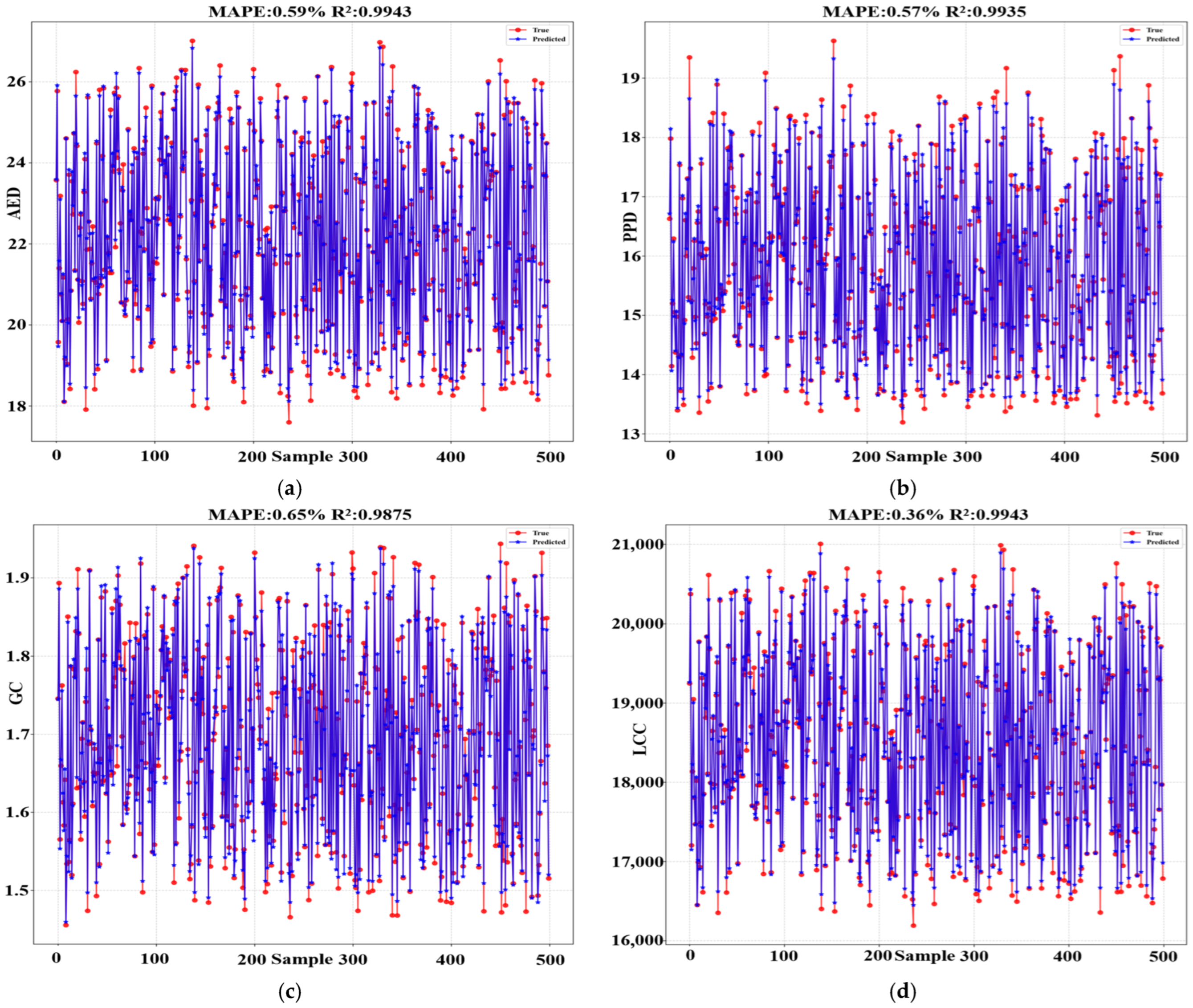
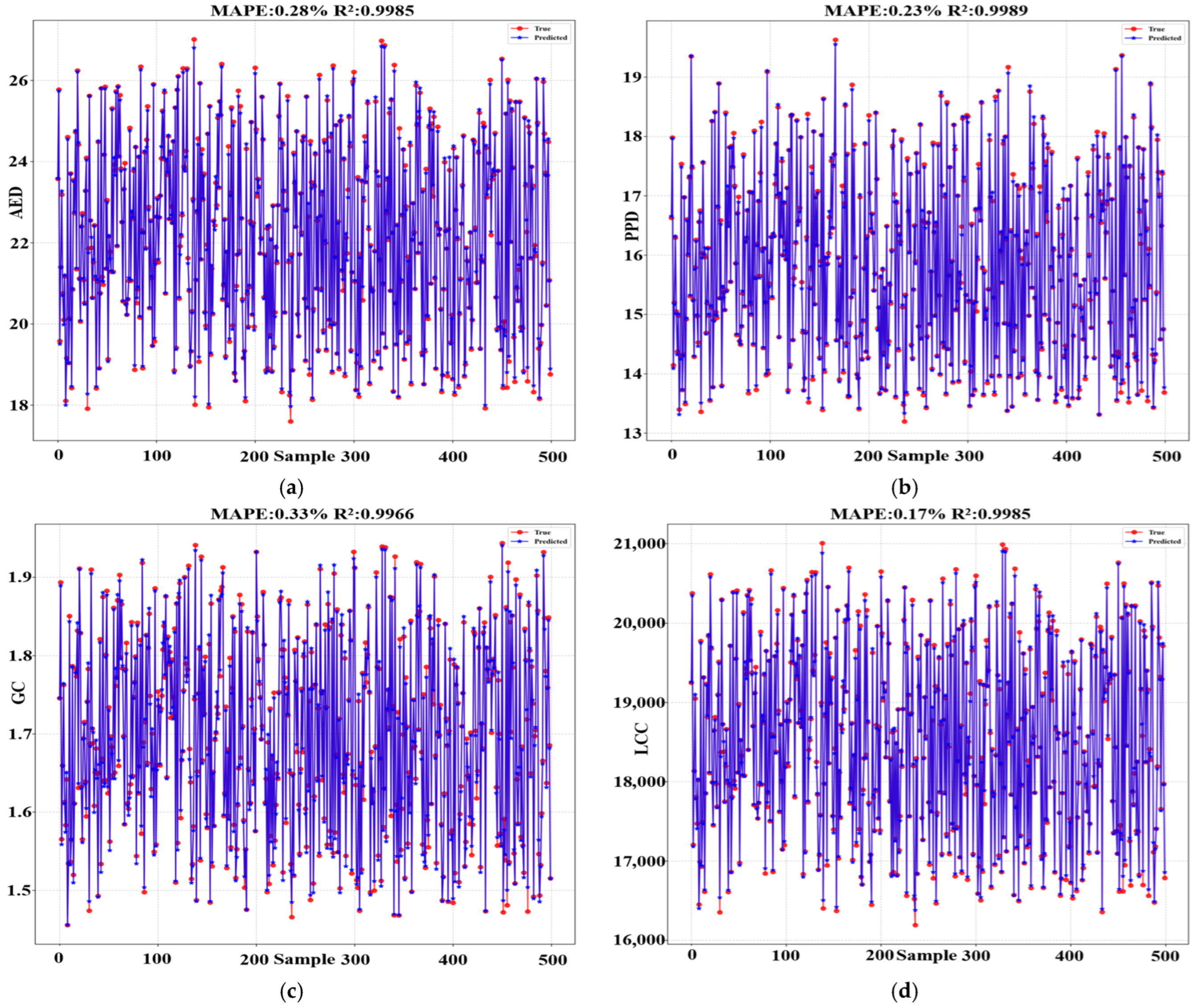
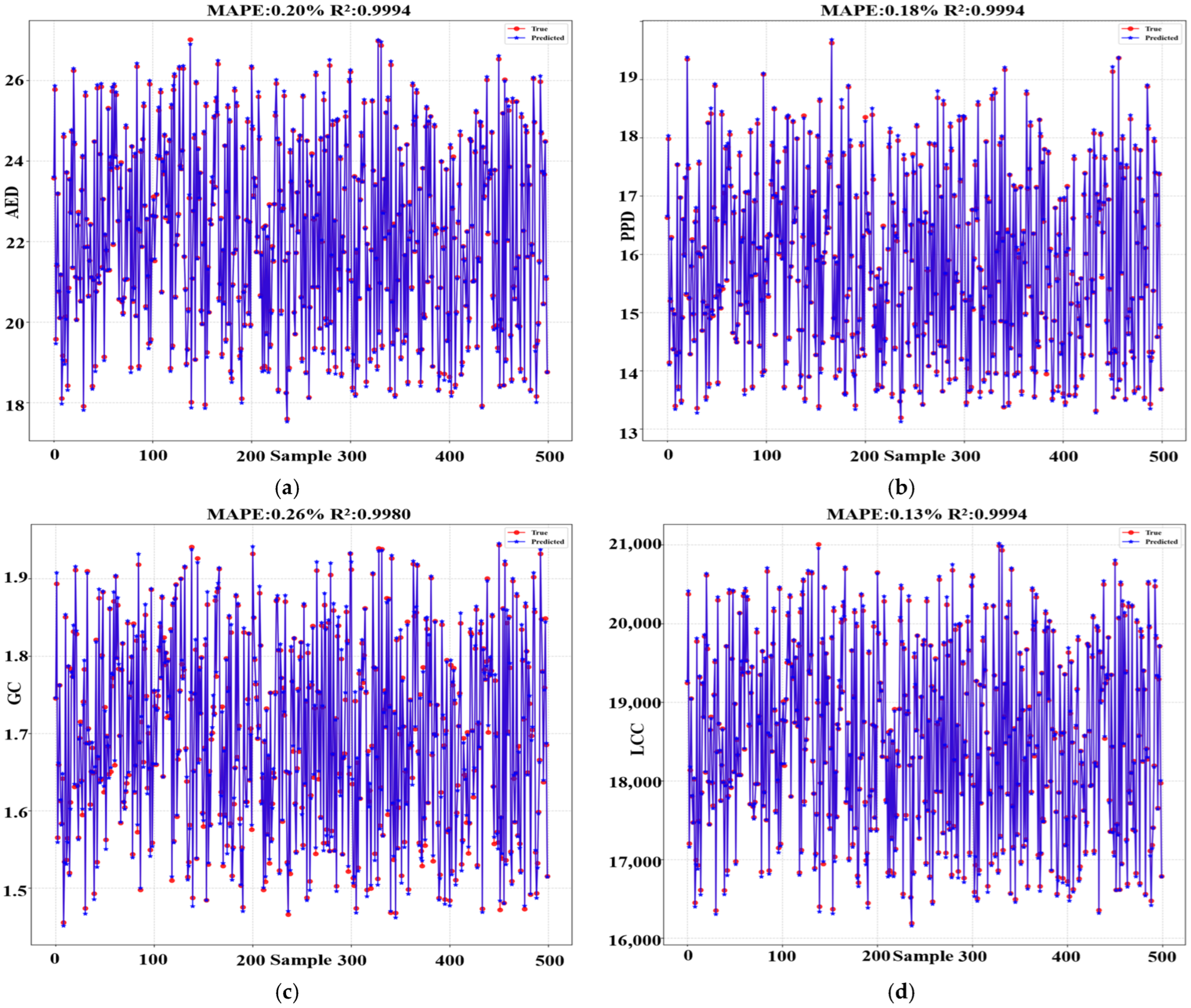
To validate the accuracy, reliability, and precision of the Transformer neural network, its performance was compared against the CNN and MLP models. The predictive accuracy of a neural network is primarily determined by its ability to generalize to unseen data; therefore, the analysis was conducted using the results from the validation set. The predictive performance for the AED, PPD, GC, and LCC achieved by the three algorithms is presented in Figure 5, Figure 6 and Figure 7, which illustrate the results for 500 uniformly sampled data points from the validation set. The coefficient of determination (R²) is a standard metric for evaluating the predictive accuracy of neural networks. A value closer to one indicates higher accuracy and a superior fit [65]. Similarly, the Mean Absolute Percentage Error (MAPE) is a critical criterion for assessing model accuracy, where a smaller value corresponds to higher predictive precision [66].

Table 5. The predictive performance of each algorithm.

Output Indicator	AED		PPD		GC		LCC
Measurement Indicator	MAPE	R2	MAPE	R2	MAPE	R2	MAPE	R2
CNN	0.59%	0.9943	0.57%	0.9935	0.65%	0.9875	0.36%	0.9943
MLP	0.28%	0.9985	0.23%	0.9989	0.33%	0.9966	0.17%	0.9985
Transformer	0.20%	0.9994	0.18%	0.9994	0.26%	0.998	0.13%	0.9994

presents the detailed results of the training for each neural network model. As illustrated in Figure 5, Figure 6 and Figure 7 and summarized in Table 5, the analysis reveals that the Transformer model demonstrated superior predictive accuracy, followed by the MLP, with the CNN exhibiting the lowest performance. The Transformer achieved the best results, as evidenced by its Mean Absolute Percentage Error (MAPE) values of 0.20%, 0.18%, 0.26%, and 0.13% for the four objectives, respectively.

The Transformer model effectively establishes nonlinear mappings between the building envelope parameters and the four optimization targets: Annual Energy Demand (AED), Predicted Percentage of Dissatisfied (PPD), Global Cost (GC), and Life Cycle Carbon (LCC). Its self-attention mechanism enables it to efficiently capture the long-range dependencies within the input sequences, making it particularly well-suited for modeling complex, high-dimensional building performance data. In summary, the Transformer presents a superior methodology for constructing surrogate models to be used as pre-screening algorithms for NSGA-III in building performance optimization.

3.4. Comprehensive MTO Evaluation

3.4.1. Analysis of the Optimization Search Results

An optimization search for the multi-objective problem involving the AED, PPD, GC, and LCC for residential buildings in Haikou was conducted using the integrated Transformer–NSGA-III framework. With four distinct objectives, this constituted a high-dimensional multi-objective optimization problem. As the dimensionality of the objective space increased, the distribution of the Pareto-optimal solutions became exponentially sparser, leading to a significant reduction in the number of non-dominated solutions [67,68]. Furthermore, a strong conflict existed between the objectives: building energy consumption and carbon emissions (AED and LCC) are typically positively correlated, while improvements in thermal comfort (PPD) often require a trade-off with the economic cost (GC). These conflicting relationships further constrained the feasible solution space. After 200 generations, the algorithm converged, yielding a final set of nine Pareto-optimal solutions.

An analysis of

Table 6. Pareto-optimal solution and common example.

Items	X1	X2	X3	X4	X5	X6	X7	X8	X9	X10	X11	AED [kWh/(m2·a)]	PPD [%]	GC [CNY]	LCC [tCO2]
1	0	0.18	0.1	0.4	0.818	0.25	2.33	0.1	0.6	0.679	1.5	17.19	12.92	14,251,495	15,976
2	0	0.18	0.1	0.4	0.818	0.25	2.33	0.1	0.6	0.732	2	17.23	12.93	14,165,846	16,015
3	0	0.18	0.1	0.4	0.818	0.25	2.33	0.1	0.6	0.679	2	17.19	12.90	14,261,677	15,974
4	10	0.18	0.1	0.4	0.818	0.25	2.33	0.1	0.6	0.732	2	17.23	12.94	14,167,325	16,019
5	0	0.18	0.1	0.4	0.818	0.25	2.685	0.08	0.6	0.806	1.5	17.27	12.99	14,085,742	16,034
6	0	0.18	0.1	0.4	0.818	0.25	2.33	0.1	0.6	0.806	2	17.23	12.93	14,157,194	16,021
7	0	0.18	0.1	0.4	0.818	0.25	2.685	0.1	0.6	0.806	1.5	17.26	12.97	14,089,298	16,036
8	0	0.25	0.1	0.4	0.818	0.25	2.685	0.08	0.6	0.806	1.5	17.28	13.05	14,063,080	16,061
9	0	0.25	0.1	0.4	0.818	0.25	2.33	0.1	0.6	0.806	1.5	17.25	13.05	14,138,820	16,045
Common example	0	0.2	0.16	0.6	0.818	0.65	2.685	0.08	0.65	0.806	1	24.07	16.99	17,719,971	19,500

indicates that the optimal solutions feature an external window construction (X7) utilizing low-emissivity (Low-e) insulating glass with argon gas fill, achieving a U-value of 1.94 W/(m²·K). This specification offers superior thermal insulation compared to the ordinary double-glazed unit in the base case. Coupled with an increase in the external sunshade projection length (X11) from 1.0 m to a range of 1.5–2.0 m, which effectively blocks direct solar radiation, the Annual Energy Demand (AED) is reduced from 24.07 kWh/(m²·a) to 17.19–17.28 kWh/(m²·a), representing a 28.5% reduction. Concurrently, the thickness of the exterior aerated concrete layer (X2) is increased from 0.20 m to 0.25 m in Solutions 8 and 9, while its thermal conductivity (X3) is maintained at the optimal value of 0.10 W/(m·K) (compared to a baseline of 0.16 W/(m·K)). These adjustments significantly lower the walls’ overall heat transfer coefficient, contributing to an optimization of the Predicted Percentage of Dissatisfied (PPD) from 16.99% to a range of 12.90–13.05%, an improvement of 24.1%. This finding is consistent with the study by Asghari et al. [69], confirming that the thermal performance of the building envelope is a decisive factor for improving energy efficiency in hot and humid regions.

It is noteworthy that the solar heat gain coefficient (X6) of the external windows is stabilized at 0.25 in all optimal solutions, which is 61.5% lower than the baseline value of 0.65. Although Li et al. [70] noted that a reduced SHGC could increase heating energy consumption, the climatic conditions in Haikou—characterized by long summers and the absence of a winter season—make the cooling load dominant. Consequently, a lower SHGC is more beneficial for reducing the air conditioning load. Furthermore, the building orientation (X1) is maintained at due south (0°), with only a 10% increase in the shading area introduced in Solution 4. This minor adjustment further enhances the energy-saving effect of the shading system by reducing the solar heat gain from the east and west. The roof configuration (X10) is optimized to an inverted design, with values between 0.679 and 0.806. This, combined with an increase in the roof insulation thickness (X8) to 0.10 m (from a baseline of 0.08 m) and a reduction in the solar absorption coefficient (X9) to 0.60 (from 0.65), helps control the initial investment while reducing the long-term operational costs. These measures collectively result in a 20.5% reduction in the Global Cost (GC) and an 18.0% reduction in the Life Cycle Carbon (LCC).

The parameter adjustments also reflect necessary design trade-offs dictated by climate adaptation. For instance, the solar absorption coefficient of the exterior walls (X4) is reduced from the baseline of 0.60 to 0.40, which suppresses the indoor temperature rise by limiting heat storage within the envelope. While the parameters related to thermal inertia, such as the 40% increase in wall thickness (X2 in Solutions 8 and 9), theoretically enhance the thermal mass, the reduction in X4 balances this by avoiding excessive heat retention in Haikou’s high-humidity environment.

Compared to the baseline case, the optimized solutions achieve the following improvements across the four objectives: a 28.5% reduction in the AED (from 24.07 to 17.19 kWh/(m²·a)); a 24.1% improvement in the PPD (from 16.99% to 12.90%); a 20.6% reduction in the GC (from CNY 17.72 to 14.06 million); and an 18.0% reduction in the LCC (from 19,500 to 15,974 tCO₂). The results demonstrate that enhanced envelope insulation and extended external shading are the principal measures for achieving a multi-objective balance in the hot and humid climate of Haikou.

3.4.2. TOPSIS Evaluation

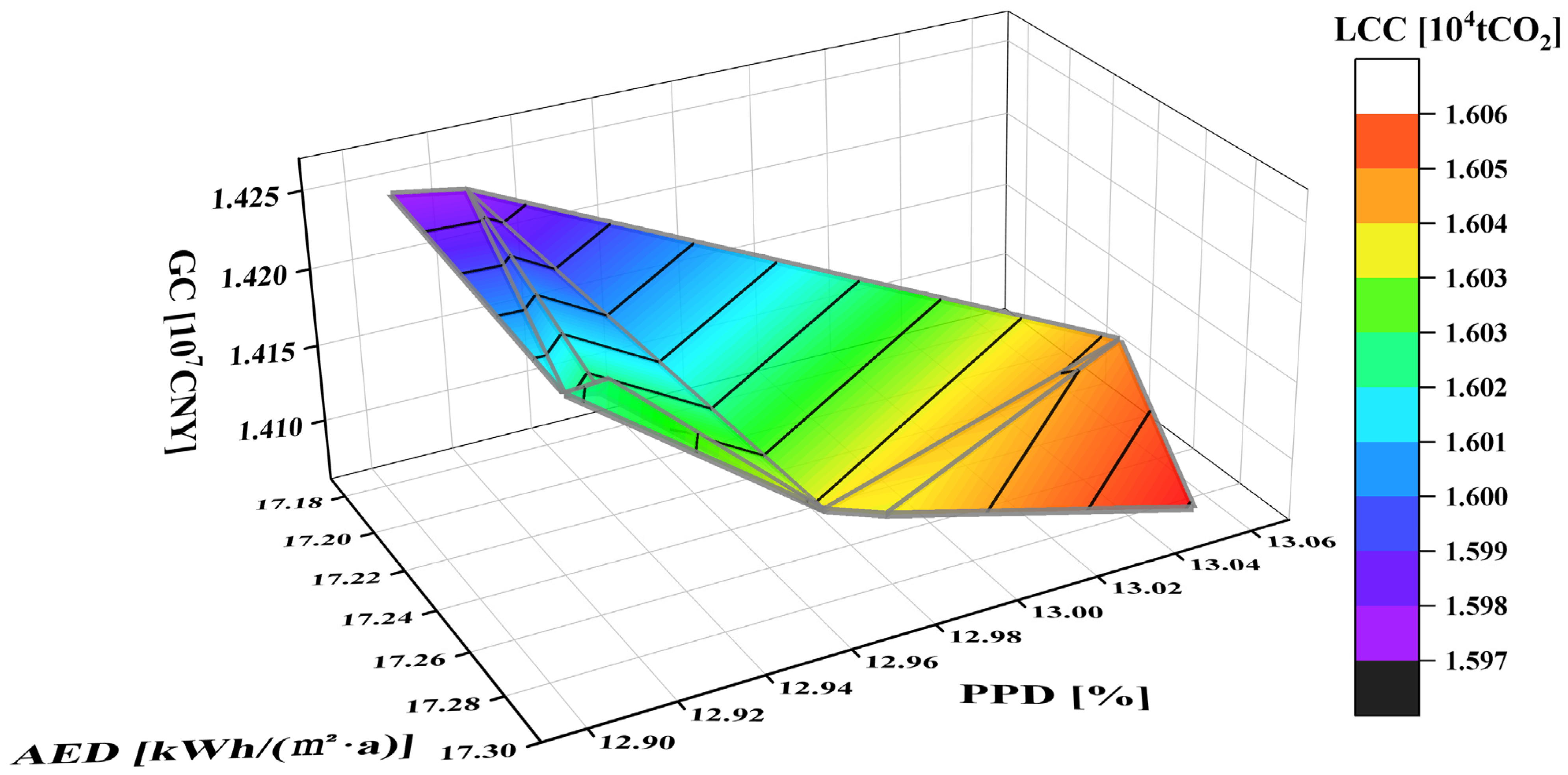
An analysis of the Pareto frontier and the TOPSIS integrated evaluation results (

Table 7. TOPSIS evaluation of optimization results.

Items	D+ (Positive Ideal Solution Distance)	D− (Negative Ideal Solution Distance)	C (Closeness)	Sort Result
1	0.501	0.917	0.647	1
2	0.474	0.646	0.577	3
3	0.523	0.957	0.647	2
4	0.497	0.615	0.553	5
5	0.717	0.539	0.429	7
6	0.485	0.639	0.568	4
7	0.653	0.568	0.465	6
8	0.957	0.523	0.353	8
9	0.813	0.39	0.324	9

and Figure 8) reveals the influence of individual parameter variations on the four objectives (AED, PPD, GC, and LCC). In the TOPSIS evaluation, equal weights of 0.25 were assigned to each objective. This equal weighting scheme provides a foundational ranking for comparing solutions; however, investigating the sensitivity of these rankings to different weight assignments constitutes an important direction for future research. The numerical labels (1–9) adjacent to each solution in Figure 8 indicate their overall ranking based on the TOPSIS comprehensive evaluation.

Based on the TOPSIS results, Solution 1 (C = 0.647) and Solution 3 (C = 0.647) achieve the highest rankings. This is attributable to the synergistic optimization of the external window configuration (X7 = 2.33 W/(m²·K)) and the external sunshade projection length (X11 = 1.5–2 m), which yields a balanced performance in both energy consumption (AED = 17.19 kWh/(m²·a)) and thermal comfort (PPD = 12.90–12.92%). In contrast, Solutions 8 (C = 0.353) and 9 (C = 0.324), despite enhancing the thermal comfort (PPD = 13.05%) by thickening the external wall insulation layer (X2 = 0.25 m), receive lower overall scores due to the higher carbon emissions associated with the roof insulation material (LCC = 16,061 tCO₂).

A cross-comparison of the solutions demonstrates that the external window insulation (X7) and external shading extension (X11) are the core parameters influencing the TOPSIS score (C-value). Their optimization can reduce the AED by up to 28.5%; however, an over-reliance on high thermal insulation, as seen in Solution 8, may exacerbate the conflict between economic and environmental objectives. A longitudinal analysis further indicates that for Haikou’s hot and humid climate, reducing the solar heat gain coefficient (X6 = 0.25) and adopting an inverted roof design (X10 = 0.679–0.806) can effectively balance heat storage and dissipation needs. For practical implementation, it is recommended to prioritize the parameter combination of Solution 1, supplemented by an intelligently adjustable shading system to dynamically adapt to seasonal changes. Furthermore, promoting the use of localized low-carbon building materials could help optimize the carbon emissions of lower-scoring solutions.

The TOPSIS evaluation provides a clear ranking of the alternatives under the defined criteria and weights. However, to enhance the practical applicability and robustness of our findings, future work must address the sensitivity of this ranking. Following the example of studies like D’Agostino et al. [71], a critical next step involves conducting a systematic sensitivity analysis on the assigned weights and testing the robustness of our conclusions against the choice of different MCDM methodologies. This will ensure that the decision-making process remains reliable under varying assumptions and stakeholder priorities.

Figure 9 illustrates the non-uniform distribution of the nine Pareto-optimal solutions within the four-dimensional objective space defined by the AED, PPD, GC, and LCC. Solutions 1 and 2 (C = 0.647) occupy optimal positions, demonstrating a superior synergy between energy efficiency and thermal comfort. In contrast, Solution 9 (C = 0.324) is located in a suboptimal region, exhibiting a compromised performance on both economic and carbon emission objectives. The morphology of the Pareto surface confirms a strong positive correlation between the AED and PPD, thereby validating the inherent trade-off between energy efficiency and occupant comfort in hot–humid climates. Conversely, the GC and LCC exhibit an approximate linear relationship, indicating significant cost barriers for implementing low-carbon technologies. This linearity suggests that substantial reductions in embodied carbon only become economically viable beyond specific investment thresholds.

4. Conclusions

This study established a Transformer–NSGA-III multi-objective optimization framework to address the interdependent challenges of energy efficiency, thermal comfort, economic cost, and Life Cycle Carbon emissions for residential buildings in Haikou’s hot–humid climate. The principal findings are summarized as follows:

• A comprehensive analysis of 79 local high-rise residences identified 11 critical envelope parameters. A sensitivity analysis revealed the external windows’ solar heat gain coefficient (X6) and external shading dimensions (X11) as the most influential factors across all the optimization objectives. The Transformer-based surrogate model demonstrated exceptional predictive accuracy for capturing the complex, nonlinear relationships between the building parameters and performance metrics, achieving R² values exceeding 0.998 for all four objectives and reducing the Mean Absolute Percentage Error (MAPE) by 40–60% compared to conventional CNN and MLP models. This high-fidelity modeling significantly accelerated the optimization process, enabling an efficient exploration of the solution space.
• The optimization results achieved substantial improvements over the baseline scenario, reducing the Annual Energy Demand (AED) by 28.5%, the Predicted Percentage of Dissatisfied (PPD) by 24.1%, the Global Cost (GC) by 20.6%, and the Life Cycle Carbon emissions (LCC) by 18.0%. The TOPSIS analysis identified Solution 1 (C = 0.647) as the most balanced Pareto-optimal solution, demonstrating the framework’s effectiveness at delivering high performance across multiple competing criteria.
• While this study provides practical design strategies for similar climatic regions, certain limitations should be acknowledged. The optimization focused primarily on the static envelope parameters; future work would benefit from incorporating dynamic operational factors and additional thermodynamic properties, such as thermal bridging coefficients. Furthermore, the Global Cost model could be enhanced by integrating more granular data from construction and demolition phases. Subsequent research will also explore the integration of subjective decision-maker preferences with objective weighting methods to generate differentiated solutions under varying stakeholder priorities.
• The proposed Transformer–NSGA-III framework demonstrates a significant transfer potential to other regions with similar hot–humid climates. Both components possess inherent advantages that support their adaptation: the Transformer architecture has proven effective at capturing complex nonlinear relationships across various domains, while NSGA-III is a well-established algorithm for high-dimensional multi-objective optimization. For successful implementation in a new location, the primary requirement would be the development of a localized dataset containing building envelope parameters and corresponding local meteorological data (in EPW format) to retrain the Transformer surrogate model, enabling it to accurately represent the specific climate–building interactions of the target region.

Notwithstanding these limitations, the proposed framework offers a robust computational foundation for navigating cost–carbon trade-offs in passive building design, presenting a viable pathway toward realizing ultra-low-energy buildings in tropical coastal regions.

References

1. Azam, A.; Ateeq, M.; Shafique, M.; Rafiq, M.; Yuan, J. Primary energy consumption-growth nexus: The role of natural resources, quality of government, and fixed capital formation. Energy 2023, 263 Pt A, 125570. [Google Scholar] [CrossRef]
2. Yang, L.; Hongyu, C. Research on factors influencing total carbon emissions of construction based on structural equation modeling: A case study from China. Build. Environ. 2025, 275, 112396. [Google Scholar] [CrossRef]
3. Liu, Y.; Chen, H.; Zhang, L.; Wu, X.; Wang, X.J. Energy consumption prediction and diagnosis of public buildings based on support vector machine learning: A case study in China. J. Clean. Prod. 2020, 272, 122542. [Google Scholar] [CrossRef]
4. Kurmanbekova, M.; Du, J.; Sharples, S. A review of indoor air quality in social housing across low-and middle-income countries. Appl. Sci. 2025, 15, 1858. [Google Scholar] [CrossRef]
5. Zhao, E.; Zhao, L.; Zhou, Z. The significance for solar heat gain on the indoor thermal environment of passive houses in cold areas in China. Energy Effic. 2020, 13, 1047–1062. [Google Scholar] [CrossRef]
6. Yin, Q.; Han, C.; Li, A.; Liu, X.; Liu, Y. A review of research on building energy consumption prediction models based on artificial neural networks. Sustainability 2024, 16, 7805. [Google Scholar] [CrossRef]
7. Hosseini, E.; Saeedpour, B.; Banaei, M.; Ebrahimy, R. Optimized deep neural network architectures for energy consumption and PV production forecasting. Energy Strateg. Rev. 2025, 59, 101704. [Google Scholar] [CrossRef]
8. Gupta, A.; Badr, Y.; Negahban, A.; Qiu, R.G. Energy-efficient heating control for smart buildings with deep reinforcement learning. J. Build. Eng. 2021, 34, 101739. [Google Scholar] [CrossRef]
9. Lin, Y.; Zhao, L.; Liu, X.; Yang, W.; Hao, X.; Tian, L. Design optimization of a passive building with green roof through machine learning and group intelligent algorithm. Buildings 2021, 11, 192. [Google Scholar] [CrossRef]
10. Jafari, A.; Valentin, V. An optimization framework for building energy retrofits decision-making. Build. Environ. 2017, 115, 118–129. [Google Scholar] [CrossRef]
11. Negendahl, K.; Nielsen, T.R. Building energy optimization in the early design stages: A simplified method. Energy Build. 2015, 105, 88–99. [Google Scholar] [CrossRef]
12. Wang, R.; Lu, S.; Feng, W. A three-stage optimization methodology for envelope design of passive house considering energy demand, thermal comfort and cost. Energy 2020, 192, 116723. [Google Scholar] [CrossRef]
13. Luo, Z.; Lu, Y.; Cang, Y.; Yang, L. Study on dual-objective optimization method of life cycle energy consumption and economy of office building based on HypE genetic algorithm. Energy Build. 2022, 256, 111749. [Google Scholar] [CrossRef]
14. Xu, Y.; Zhang, G.; Yan, C.; Wang, G.; Jiang, Y.; Zhao, K. A two-stage multi-objective optimization method for envelope and energy generation systems of primary and secondary school teaching buildings in China. Build. Environ. 2021, 204, 108142. [Google Scholar] [CrossRef]
15. Chen, B.; Liu, Q.; Chen, H.; Wang, L.; Deng, T.; Zhang, L.; Wu, X. Multiobjective optimization of building energy consumption based on BIM-DB and LSSVM-NSGA-II. J. Clean. Prod. 2021, 294, 126153. [Google Scholar] [CrossRef]
16. Gou, S.; Nik, V.M.; Scartezzini, J.L.; Zhao, Q.; Li, Z. Passive design optimization of newly-built residential buildings in Shanghai for improving indoor thermal comfort while reducing building energy demand. Energy Build. 2018, 169, 484–506. [Google Scholar] [CrossRef]
17. Al Mindeel, T.; Spentzou, E.; Eftekhari, M. Energy, thermal comfort, and indoor air quality: Multi-objective optimization review. Renew. Sustain. Energy Rev. 2024, 202, 114682. [Google Scholar] [CrossRef]
18. Alimohamadi, R.; Jahangir, M.H. Multi-Objective optimization of energy consumption pattern in order to provide thermal comfort and reduce costs in a residential building. Energy Convers. Manag. 2024, 305, 118214. [Google Scholar] [CrossRef]
19. Wu, C.; Pan, H.; Luo, Z.; Liu, C.; Huang, H. Multi-objective optimization of residential building energy consumption, daylighting, and thermal comfort based on BO-XGBoost-NSGA-II. Build. Environ. 2024, 254, 111386. [Google Scholar] [CrossRef]
20. Benaddi, F.Z.; Boukhattem, L.; Tabares-Velasco, P.C. Multi-objective optimization of building envelope components based on economic, environmental, and thermal comfort criteria. Energy Build. 2024, 305, 113909. [Google Scholar] [CrossRef]
21. Canbolat, A.S.; Albak, E.I. Multi-objective optimization of building design parameters for cost reduction and CO2 emission control using four different algorithms. Appl. Sci. 2024, 14, 7668. [Google Scholar] [CrossRef]
22. Chen, R.; Tsay, Y.S.; Zhang, T. A multi-objective optimization strategy for building carbon emission from the whole life cycle perspective. Energy 2023, 262, 125373. [Google Scholar] [CrossRef]
23. Kang, Y.; Zhang, D.; Cui, Y.; Xu, W.; Lu, S.; Wu, J.; Hu, Y. Integrated passive design method optimized for carbon emissions, economics, and thermal comfort of zero-carbon buildings. Energy 2024, 295, 131048. [Google Scholar] [CrossRef]
24. Ma, H.; Zhang, Y.; Sun, S.; Liu, T.; Shan, Y. A comprehensive survey on NSGA-II for multi-objective optimization and applications. Artif. Intell. Rev. 2023, 56, 15217–15270. [Google Scholar] [CrossRef]
25. Deb, K.; Pratap, A.; Agarwal, S.; Meyarivan, T. A fast and elitist multiobjective genetic algorithm: NSGA-II. IEEE Trans. Evol. Comput. 2002, 6, 182–197. [Google Scholar] [CrossRef]
26. Schaffer, J.D. Multiple objective optimization with vector evaluated genetic algorithms. In Proceedings of the First International Conference on Genetic Algorithms and Their Applications, Pittsburgh, PA, USA, 1 July 1985; pp. 93–100. [Google Scholar]
27. Fonseca, C.M.; Fleming, P.J. Genetic algorithms for multiobjective optimization: Formulation discussion and generalization. In Proceedings of the 5th International Conference on Genetic Algorithms, Urbana-Champaign, IL, USA, 17–21 July 1993; pp. 416–423. [Google Scholar]
28. Horn, J.; Nafpliotis, N.; Goldberg, D.E. Multiobjective Optimization Using the Niched Pareto Genetic Algorithm; University of Illinois at Urbana-Champaign: Urbana, IL, USA, 1993. [Google Scholar]
29. Srinivas, N.; Deb, K. Muiltiobjective optimization using nondominated sorting in genetic algorithms. Evol. Comput. 1994, 2, 221–248. [Google Scholar] [CrossRef]
30. Jain, H.; Deb, K.; Jain, H.; Deb, K. An evolutionary many-objective optimization algorithm using reference-point based nondominated sorting approach, part II: Handling constraints and extending to an adaptive approach. IEEE Trans. Evol. Comput. 2014, 18, 602–622. [Google Scholar] [CrossRef]
31. Zitzler, E.; Thiele, L. Multiobjective evolutionary algorithms: A comparative case study and the strength Pareto approach. IEEE Trans. Evol. Comput. 1999, 3, 257–271. [Google Scholar] [CrossRef]
32. Zitzler, E.; Laumanns, M.; Thiele, L. SPEA2: Improving the Strength Pareto Evolutionary Algorithm for Multiobjective Optimization; ETH Zurich: Zurich, Switzerland, 2001. [Google Scholar]
33. Zhan, J.; He, W.; Huang, J. Comfort, carbon emissions, and cost of building envelope and photovoltaic arrangement optimization through a two-stage model. Appl. Energy 2024, 356, 122423. [Google Scholar] [CrossRef]
34. Rafati, N.; Hazbei, M.; Eicker, U. Louver configuration comparison in three Canadian cities utilizing NSGA-II. Build. Environ. 2023, 229, 109939. [Google Scholar] [CrossRef]
35. Cheraghi, R.; Jahangir, M.H. Multi-objective optimization of a hybrid renewable energy system supplying a residential building using NSGA-II and MOPSO algorithms. Energy Convers. Manag. 2023, 294, 117515. [Google Scholar] [CrossRef]
36. Baghoolizadeh, M.; Rostamzadeh-Renani, M.; Rostamzadeh-Renani, R.; Toghraie, D. Multi-objective optimization of Venetian blinds in office buildings to reduce electricity consumption and improve visual and thermal comfort by NSGA-II. Energy Build. 2023, 278, 112639. [Google Scholar] [CrossRef]
37. Peng, J.; Feng, Y.; Zhang, Q.; Liu, X. Multi-objective integrated optimization study of prefabricated building projects introducing sustainable levels. Sci. Rep. 2023, 13, 2821. [Google Scholar] [CrossRef]
38. Lu, Y.; Wang, S.; Zhao, Y.; Yan, C. Renewable energy system optimization of low/zero energy buildings using single-objective and multi-objective optimization methods. Energy Build. 2015, 89, 61–75. [Google Scholar] [CrossRef]
39. Opris, A.; Dang, D.C.; Neumann, F.; Sudholt, D. Runtime analyses of NSGA-III on many-objective problems (Version 2). In Proceedings of the Genetic and Evolutionary Computation Conference, Melbourne, VIC, Australia, 14–18 July 2024; pp. 1596–1604. [Google Scholar] [CrossRef]
40. Wu, X.; Li, X.; Qin, Y.; Xu, W.; Liu, Y. Intelligent multiobjective optimization design for NZEBs in China: Four climatic regions. Appl. Energy 2023, 339, 120934. [Google Scholar] [CrossRef]
41. Vaswani, A.; Shazeer, N.; Parmar, N.; Uszkoreit, J.; Jones, L.; Gomez, A.N.; Kaiser, L.U.; Polosukhin, I. Attention is all you need. In Proceedings of the 31st International Conference on Neural Information Processing Systems, Long Beach, CA, USA, 4–9 December 2017; pp. 6000–6010. [Google Scholar] [CrossRef]
42. Clemente, A.V.; Nocente, A.; Ruocco, M. Global transformer architecture for indoor room temperature forecasting. J. Phys. Conf. Ser. 2023, 2600, 022018. [Google Scholar] [CrossRef]
43. Spencer, R.; Ranathunga, S.; Boulic, M.; Van Heerden, A.H.; Susnjak, T. Transfer learning on transformers for building energy consumption forecasting—A comparative study. Energy Build. 2025, 336, 115632. [Google Scholar] [CrossRef]
44. Xu, Y.; Yang, Y.; Zhang, L. DeMT: Deformable mixer transformer for multi-task learning of dense prediction. In Proceedings of the AAAI Conference on Artificial Intelligence, Washington, DC, USA, 7–14 February 2023; pp. 3072–3080. [Google Scholar] [CrossRef]
45. Huo, H.; Deng, X.; Wei, Y.; Liu, Z.; Liu, M.; Tang, L. Optimization of energy-saving renovation technology for existing buildings in a hot summer and cold winter area. J. Build. Eng. 2024, 86, 108597. [Google Scholar] [CrossRef]
46. Xiang, J.; Liu, H.; Li, X.; Jones, P.; Perisoglou, E. Multi-objective optimization of ultra-low energy housing in hot summer cold winter climate zone of China based on a probabilistic behavioral model. Buildings 2023, 13, 1172. [Google Scholar] [CrossRef]
47. Qian, F.; Sun, H.; Yang, L. Integrating smart city principles in the numerical simulation analysis on passive energy saving of small and medium gymnasiums. Smart Cities 2024, 7, 1971–1991. [Google Scholar] [CrossRef]
48. Harkouss, F.; Fardoun, F.; Biwole, P.H. Passive design optimization of low energy buildings in different climates. Energy 2018, 165, 591–613. [Google Scholar] [CrossRef]
49. Tartarini, F.; Schiavon, S. Comparative Analysis of PMV Models Accuracy Implemented in the ISO 7730:2005 and ASHRAE 55:2023. Build. Environ. 2025, 275, 112766. [Google Scholar] [CrossRef]
50. Buildings Performance Institute Europe. Cost Optimality—Discussing Methodology and Challenges Within the Recast. 2010. Available online: http://www.buildup.eu/sites/default/files/content/BPIE_costoptimality_publication2010.pdf (accessed on 29 April 2023).
51. Wang, Y.; Hu, L.; Hou, L.; Cai, W.; Wang, L.; He, Y. Study on energy consumption, thermal comfort and economy of passive buildings based on multi-objective optimization algorithm for existing passive buildings. J. Clean. Prod. 2023, 425, 138760. [Google Scholar] [CrossRef]
52. Wu, Z. Application of CNN classic model in modern image processing. J. Adv. Eng. Technol. 2024, 1, 1–6. [Google Scholar] [CrossRef]
53. Liu, X.; Gao, P.; Yu, T.; Wang, F.; Yuan, R.Y. CSWin-UNet: Transformer UNet with cross-shaped windows for medical image segmentation. Inform. Fusion 2025, 113, 102634. [Google Scholar] [CrossRef]
54. Lei, R.; Cheng, Y. A pareto-based differential evolution algorithm for multi-objective optimization problems. In Proceedings of the 2010 Chinese Control and Decision Conference, Xuzhou, China, 26–28 May 2010; pp. 1608–1613. [Google Scholar] [CrossRef]
55. Wan, C.; Niu, M.; Song, Y.; Xu, Z. Pareto optimal prediction intervals of electricity price. IEEE Trans. Power Syst. 2016, 32, 817–819. [Google Scholar] [CrossRef]
56. Zheng, W.; Doerr, B. Better approximation guarantees for the NSGA-II by using the current crowding distance. In Proceedings of the Genetic and Evolutionary Computation Conference, Boston, MA, USA, 9–13 July 2022; pp. 611–619. [Google Scholar]
57. Hu, Y.; Wu, L.; Shi, C.; Wang, Y.; Zhu, F. Research on optimal decision-making of cloud manufacturing service provider based on grey correlation analysis and TOPSIS. Int. J. Prod. Res. 2020, 58, 748–757. [Google Scholar] [CrossRef]
58. Kannan, V.S.; Navneethakrishnan, P. Machining parameters optimization in laser beam machining for micro elliptical profiles using TOPSIS method. Mater. Today Proc. 2020, 21 Pt 1, 727–730. [Google Scholar] [CrossRef]
59. GB 55015-2021; General Code for Energy Efficiency and Renewable Energy Application in Buildings. State Administration for Market Regulation: Beijing, China, 2021.
60. GB/T 50785-2012; Evaluation Standard for Indoor Thermal and Humidity Environment of Civil Buildings. China Architecture & Building Press: Beijing, China, 2012.
61. Wang, Y.; Hou, L.; Cai, W.; Zhou, Z.; Bian, J. Exploring the drivers and influencing mechanisms of urban household electricity consumption in China-based on longitudinal data at the provincial level. Energy 2023, 273, 127191. [Google Scholar] [CrossRef]
62. Gundogdu, O.; Egrioglu, E.; Aladag, C.H.; Yolcu, U. Multiplicative neuron model artificial neural network based on Gaussian activation function. Neural Comput. Appl. 2016, 27, 927–935. [Google Scholar] [CrossRef]
63. Kiatkaiwansiri, T.; Sinthupinyo, S. Combining nodes in multiple neural network on large datasets. In Proceedings of the 2014 Fourth International Conference on Digital Information and Communication Technology and its Applications (DICTAP), Bangkok, Thailand, 6–8 May 2014; pp. 28–30. [Google Scholar] [CrossRef]
64. Zhang, Y.; Zhou, C.; Liu, M.; Li, X.; Liu, T.; Liu, Z. Thermal insulation performance of buildings with phase-change energy-storage wall structures. J. Clean. Prod. 2024, 438, 140749. [Google Scholar] [CrossRef]
65. Wang, Y.; Lin, M.; Gao, J.; Zhou, Z. Fading attraction of the shrinking city: An empirical study from an urban resource perspective. Sustainability 2021, 13, 11550. [Google Scholar] [CrossRef]
66. Gao, Q.J.; Zhou, Y.C.; Zhao, S.Q.; Zhang, S.Y. Comparison on predictive capacity of ARIMA model and LSTM model for incidence of hand, foot and mouth disease in Shijiazhuang. Chin. J. Dis. Control Prev. 2020, 24, 73–78. [Google Scholar] [CrossRef]
67. Opris, A. A first runtime analysis of NSGA-III on a many-objective multimodal problem: Provable exponential speedup via stochastic population update (Version 1). arXiv 2025. [Google Scholar] [CrossRef]
68. Utyuzhnikov, S. Extension of the Directed Search Domain algorithm for multi-objective optimization to higher dimensions. Ann. Oper. Res. 2024, 340, 1125–1160. [Google Scholar] [CrossRef]
69. Asghari, M.; Fereidoni, S.; Fereidooni, L.; Nabisi, M.; Kasaeian, A. Energy efficiency analysis of applying phase change materials and thermal insulation layers in a building. Energy Build. 2024, 312, 114211. [Google Scholar] [CrossRef]
70. Li, J.; Wu, J.; Xu, H. Effect of photovoltaic energy-saving window factors on building heating load under three control modes. Buildings 2025, 15, 238. [Google Scholar] [CrossRef]
71. D’Agostino, D.; Minelli, F.; Minichiello, F. An innovative multi-stakeholder decision methodology for the optimal energy retrofit of shopping mall buildings. Energy Build. 2025, 344, 115958. [Google Scholar] [CrossRef]
72. JGJ/T 17-2008; Technical Specification for Architectural Application of Autoclaved Aerated Concrete. China Architecture & Building Press: Beijing, China, 2009.
73. GB 55007-2021; General Standard for Masonry Structures. China Architecture & Building Press: Beijing, China, 2021.
74. GB 50176-2016; Code for Thermal Design of Civil Building. China Architecture & Building Press: Beijing, China, 2016.
75. GB/T 30595-2024; Extruded Polystyrene (XPS) Board System for Building Thermal Insulation. State Administration for Market Regulation, Standardization Administration: Beijing, China, 2024.
76. JGJ 75-2012; Design Standard for Energy Efficiency of Residential Buildings in Hot Summer and Warm Winter Zone. Ministry of Housing and Urban-Rural Development of the People’s Republic of China: Beijing, China, 2012.
77. JGJ 237-2011; Technical Specification for Building Shading Engineering. Ministry of Housing and Urban-Rural Development of the People’s Republic of China: Beijing, China, 2011.
Figure 1. The research framework.
Buildings 15 03939 g001
Figure 2. Survey results of building orientation and building floors. (a) Building orientation distribution; (b) building layer distribution.
Buildings 15 03939 g002
Figure 3. Point building floorplan.
Buildings 15 03939 g003
Figure 4. Flowchart of NSGA-III.
Buildings 15 03939 g004
Figure 5. The training results of the CNN on the four-objective prediction set. (a) Training results for AED based on CNN; (b) training results for PDD based on CNN; (c) training results for GC based on CNN; (d) training results for LCC based on CNN.
Buildings 15 03939 g005
Figure 6. The training results of the MLP neural network on the four-objective prediction set. (a) Training results for AED based on MLP; (b) training results for PDD based on MLP; (c) training results for GC based on MLP; (d) training results for LCC based on MLP.
Buildings 15 03939 g006
Figure 7. The training results of the Transformer neural network on the four-objective prediction set. (a) Training results for AED based on Transformer; (b) training results for PDD based on Transformer; (c) training results for GC based on Transformer; (d) training results for LCC based on Transformer.
Buildings 15 03939 g007
Figure 8. Pareto front calculation results.
Buildings 15 03939 g008
Figure 9. Pareto surface.
Buildings 15 03939 g009