Abstract
Digital Twins rely on accurate geometric models to ensure reliable representation, yet maintaining and updating these models remains a persistent challenge. This paper addresses one aspect of this challenge by focusing on the verification of photogrammetry-based models. It introduces a verification framework that defines measurable data quality elements and establishes conditions to assess whether model quality is maintained, improved, or degraded. Validation through a university building case study demonstrates the framework’s ability to detect quality differences between visually similar models. Meeting only one of the three verification conditions, the new model shows quality degradation, primarily due to reduced positional accuracy and resolution, making it unsuitable to replace the previous version used in the Digital Twin. Additionally, the developed web tool prototype enables the automated calculation of the framework’s verification scores. This study contributes to the growing discussion on Digital Twin maintenance by providing practical insights for improving the reliability of geometric models.
1. Introduction
Digital Twin technology has gained substantial attention in recent years, finding applications across diverse domains. At its core, a Digital Twin consists of three elements: the physical object (Physical Twin), its virtual representation (Digital Twin), and the bidirectional flow of data (Digital Thread) enabled by IoT devices [1]. The concept was first introduced by Dr. Michael W. Grieves at a Society of Manufacturing Engineering conference in October 2002 [2]. At that time, he described it as the “Conceptual Ideal for Product Lifecycle Management,” as the term “Digital Twin” had not yet been coined. The naming evolved over the years—from the “Mirrored Spaces Model” in 2005 to the “Information Mirroring Model” in 2006—before the term “Digital Twin” was formally adopted in 2010 during collaboration with NASA.
Researchers and industry practitioners have since identified various requirements for Digital Twins, including maturity levels [3,4], automation and autonomy [5], data integration [6], and learning capabilities [7,8]. Although a Digital Twin can never fully replicate its real-world counterpart, particularly in complex settings, it is designed to capture the essential characteristics of the physical environment and leverage collected data for service delivery or task optimization.
In the built environment, a Digital Twin is often defined as a digital replica of a building or infrastructure that functions as a central information repository, supporting storage, analysis, sharing, and service provision [1,9]. Services are typically defined based on the specific aspects or processes that need optimization. While developing a complex information system for simple tasks is rarely justified, implementing a Digital Twin becomes practical for complex assets or repetitive processes where the cost of information is lower than the cost of physical testing or wasted resources. ISO/IEC 30173:2023 provides examples of such services, including state analysis, simulation, and performance optimization [10].
The term “Geometric Digital Twin” (GDT) refers specifically to a 3D representation of the Physical Twin without incorporating semantic or relational information [11]. Creating or updating a GDT relies on Spatial and Visual Data (SVD) [12,13,14]. SVD includes point clouds, classified as spatial data, and images or video sequences, classified as visual data, typically captured using terrestrial or mobile scanners and cameras.
In university settings, Digital Twin supports a wide range of users. A small group, such as developers and operators, engages with the system at a technical level, while the broader community of students, staff, and visitors interacts with its services. These services include environmental visualization for orientation and navigation, as well as predictive maintenance of campus buildings and infrastructure to reduce operational costs. Within this context, the geometry of the Digital Twin is particularly important since it provides the spatial foundation upon which these services are built.
Photogrammetric models offer significant potential for creating campus-scale Digital Twins. Advances in image-based 3D scene capture have made it possible to generate detailed and textured models using even low-cost sensors such as smartphone cameras and Unmanned Aerial Vehicles (UAVs) [15]. Despite these advancements, errors can still occur during data collection, preprocessing, and modeling. Inaccuracies in geometric models can lead to spatial misalignment of data and unreliable visualization and analysis, directly affecting daily operations and long-term facility management on campus. Consequently, verifying model quality remains a critical and ongoing challenge, serving as a necessary precondition for the maintenance and updating of Digital Twins.
This paper addresses a specific aspect of this challenge by focusing on the verification of photogrammetry-based models. The research question is as follows: “How can the quality of a geometric model (the candidate model replacing an earlier version in the Digital Twin) be verified, and what workflow and conditions are required to support the verification process for long-term use?”. Therefore, the contributions of this paper are as follows:
- It defines measurable data quality elements for geometric model verification.
- It formulates explicit conditions for determining whether a geometric model maintains, improves, or degrades in quality.
- It provides a verification tool to calculate the scores and streamline the process.
The paper is organized as follows. The Background section reviews Digital Twin applications in university environments, current evaluation approaches, and data acquisition and measurement errors, as well as the accuracy and Level of Detail (LoD) of photogrammetry-based models. The Research Methodology section outlines the approach used for developing the framework, followed by the Framework for Verification of Geometric Digital Twins section, which presents the framework itself. The Results section demonstrates the framework’s implementation in a case study. The Discussion section reflects on the framework results, assesses them via alternative approaches, and highlights limitations and directions for future research. Finally, Appendix A and Appendix B provide detailed case study descriptions and present the prototype web application used for calculations.
2. Background
2.1. Digital Twins in University Environments
With growing interest in Digital Twin and its broad range of applications, many universities are investing in exploring, testing, and implementing technology to improve their environments and processes. At the University of Galway (Ireland), a 3D campus model was developed using surveys, photogrammetry, and façade photography [16]. The model was further enhanced with gaming technology to simulate dynamic shadows and weather effects. The goal of this creation was to support master planning, provide visualizations, and assist in traffic and pedestrian flow management. Although the system does not integrate real-time data and only provides spatial information, it can be considered a GDT for the campus environment.
At Western Sydney University (Australia), a Digital Twin is used to maintain the library by optimizing indoor environmental conditions, such as temperature, humidity, lighting, CO2 levels, and TVOC concentration [17]. The system integrates a BIM model with a sensor network and is structured around a four-layer architecture: (1) data acquisition, (2) data communication and storage, (3) data and BIM integration, and (4) data analysis and visualization using semiotic representation. Although there are limitations, such as limited sensor coverage and an absence of performance simulations over time, the study emphasizes the practical application of Digital Twin technology in a university setting.
A dynamic Digital Twin was developed to support facility management at the Institute for Manufacturing, University of Cambridge (United Kingdom) [18]. The system integrates a BIM model, the building management system, and real-time sensor data, including temperature, humidity, lighting, CO2, vibration, and occupancy monitoring. Its architecture consists of five layers: (1) data acquisition, (2) transmission, (3) digital modeling and data enhancement, (4) data-model integration, and (5) application. The study shows that a medium level of model accuracy (CityGML LoD 2–3 for the building and LoD 4 for specific areas or systems) is sufficient for supporting building maintenance.
A Digital Twin-based smart campus system was developed at Hubei University of Technology (China) [19]. The architecture combines a static spatial model with a dynamic data model. The static model includes a 3D representation of the environment, a behavioral model, and a set of simulation rules. The spatial data is organized in typical GIS layers such as terrain, roads, buildings, vegetation, and water. The dynamic model focuses mainly on synthetic simulation data, incorporating virtual and augmented reality. However, at the stage described in the study, the Digital Twin served primarily as a visualization and had not yet incorporated real-time sensor data.
The University of Birmingham (United Kingdom) illustrates another approach to developing a smart campus [20]. The campus is presented through 360-degree views and photographs of key locations, including accommodation, academic buildings, and nearby urban facilities, with some buildings offering internal virtual tours. A similar visualization approach is used at Georgetown University (USA) [21], where 2D maps include a comprehensive set of points of interest such as campus entrances, academic and residential buildings, parking and transportation, ADA facilities, sustainability initiatives, and virtual tours. Table 1 summarizes Digital Twin applications in universities and indicates that the technology is still in its early stages, with limited integration of real-time data and a primary focus on visualization. Although traditional maps and photographs are still widely used, the increasing volume of data and advancing technology will likely lead to the adoption of more sophisticated approaches.

Table 1.
Overview of Digital Twin applications in universities.
2.2. Evaluation of Digital Twins
In the context of assessing the geometric models used in Digital Twins, there is currently no universally applicable evaluation framework. Since no single geometric representation can accommodate the diverse use cases of a Digital Twin, requirements for geometry representation and assessment are typically defined based on the specific needs of each application.
The geometric accuracy of Digital Twins for bridges generated from point clouds was analyzed in [22]. The study examines strategies to achieve the required Level of Geometric Accuracy (LOGA) and emphasizes the need for an evaluation framework to support twinning and model updates. The study highlights that elements of different scales may require distinct twinning techniques, and a single Digital Twin may, therefore, include multiple types of geometric representations. To address this, the authors propose a two-level approach: at the macro-level, deviations are assessed to identify broad areas with significant discrepancies, often caused by occlusion or noise during data acquisition; at the micro-level, deviations are analyzed at the component scale for detailed accuracy evaluation. The case study evaluates the accuracy of the model by summing errors from the laser scanner and the scanning and modeling processes. However, it does not analyze these errors separately or suggest ways to reduce them. Instead, it focuses on the aggregated value of the model’s represented accuracy. The study also reviews the models’ classification systems (Level of Development, Level of Detail, Level of Information, and Model Granularity), which are mostly design-focused and less adaptive for as-built models.
The concept of “Level of As-Is Detail” for Digital Twins of roads was introduced in [23], emphasizing the need for an evaluation framework for assets in the Use phase. The concept includes the Level of Geometric Representation (LoGR) and Level of Semantic Granularity (LoSG), as well as two sub-concepts: Level of Geometric Uncertainty (LoGU), reflecting the accuracy of geometric reconstruction, and Level of Semantic Uncertainty (LoSU), indicating the reliability of object classification. However, this concept is domain-specific and lacks quantitative assessment metrics. Similarly, a grading system for twinning heritage buildings from point clouds was proposed in [24], comprising the Grade of Generation (GoG) to capture model scale, the Grade of Information (GoI) for informational requirements, and the Grade of Accuracy (GoA) to classify deviations between the point cloud and BIM model. GoA is quantified using mean distance, median, and standard deviation. However, the study focuses primarily on the modeling process and relies on the BIM model as the reference baseline, which may not always be available for buildings in the Use stage.
Several studies highlight the importance of updating GDT [12,14,25]. The concept of Geometric Coherence, which measures the similarity between the geometries of Physical and Digital Twins, has also been introduced in [25]. Maintaining coherence requires detecting changes in the physical object before updating its digital counterpart. While the study emphasizes geometry updating, it provides no concrete guidelines, focusing instead on the types of geometric changes and technologies for capturing them. Current SVD-based approaches for updating GDT have been reviewed in [14], and a geometry-based object class hierarchy was proposed to support the updating process. In that study, geometry updating is considered part of the ongoing maintenance of Digital Twins throughout the building lifecycle, with a primary focus on the Construction and Use phases. Subsequent research provided a more detailed review of methods for constructing and maintaining the as-is geometry of building Digital Twins [12]. However, both studies primarily rely on point clouds and use the BIM model as a reference. Their review of image-based methods focused on CNN-based object detection, which enables the identification of frequently occurring objects and those requiring substantial digitization effort. While effective for models with object classification, the approach is less relevant when classification is absent or incomplete.
2.3. Data Acquisition and Measurement Errors
The construction of a GDT relies on data collected under a set of interrelated conditions (“complex of conditions”): the object (what is measured), the subject (who measures), equipment (measured by), method (how measured), and environment (where measured). Optimizing these conditions enhances data accuracy, while suboptimal conditions increase the likelihood of errors. During geometry updates, individual elements can be adjusted, but full consistency cannot be guaranteed. Figure 1 illustrates the main factors influencing data acquisition accuracy, including the complex of conditions, measurements, and error types.
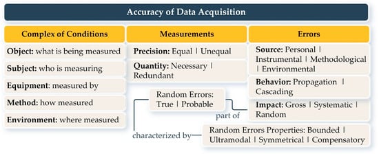
Figure 1.
The main factors affecting data acquisition accuracy.
According to the theory of measurement errors and uncertainties, measurements can be obtained either directly or indirectly (derived through calculations based on other measured values) [26]. In terms of precision, measurements can be of equal precision, conducted under nearly identical conditions (rare in practice), or of unequal precision, taken under varying conditions (more common). The numerical values of the errors of equal-precision measurements can be estimated based on the Arithmetic Mean, Mean Square Error, and the Mean Square Error of the Arithmetic Mean. Unequal-precision measurements are evaluated using Measurement Weights, the Weighted Arithmetic Mean, and the Mean Square Error of a Unit Weight.
Based on the source, the errors in measurements can be classified as follows:
- Instrument errors: Imperfect design of the equipment;
- Personal errors: Caused by the observer’s condition during work;
- External errors: Changes in the environment during the data collection;
- Methodological errors: Incomplete consideration of conditions or incorrect methodological approach.
In terms of quantity, the measurements can be necessary or redundant, where redundancy refers to additional measurements beyond the required minimum. Based on impact, the errors in measurements can be classified as follows:
- Gross errors: Large deviations exceeding permissible limits;
- Systematic errors: Appear in all measurements and follow a pattern, either constant or variable;
- Random errors: Caused by variations in conditions; they cannot be completely eliminated, but can be assessed through redundant measurements.
Systematic and random errors are both common and significant, capable of propagating from one error to another or cascading undetected.
To improve consistency in data acquisition and reduce errors during geometry updating, Table 2 organizes acquisition variables along two dimensions: measurability (whether a variable can be quantified) and controllability (whether it can be adjusted).
Table 2.
Classification of the data acquisition variables.
- Measurable and Controllable: Includes factors such as the measured object and measurement type (precision, quantity). These can be monitored and adjusted to ensure consistency across datasets (e.g., survey scope, coverage area, flight pattern, lighting).
- Measurable but Not Controllable: Refers to error sources, impacts, and behaviors that can be quantified and partly mitigated during data processing but not directly controlled during data acquisition.
- Controllable but Not Measurable: Refers to equipment calibration and consistent acquisition methods to reduce the occurrence of systematic errors.
- Not Measurable and Not Controllable: Includes the operator and environmental conditions, which cannot be quantified or controlled and may introduce gross or random errors.
2.4. Model Accuracy and Level of Detail
Accuracy refers to the extent to which the information in a model aligns with accepted or true values, making it a critical parameter for evaluating geometric models. Accuracy reflects overall data quality and the presence of errors, and it is typically assessed in terms of completeness, consistency, positional accuracy, and temporal quality [27]. Accuracy should not be confused with precision, which relates to the measurements taken during data acquisition [28]. High precision does not guarantee high accuracy, nor vice versa. Model accuracy is typically categorized into two types: measured accuracy, based on the standard deviation of raw measurements, and represented accuracy, based on the processed data.
Model accuracy is also independent of LoD; any LoD can be achieved at varying accuracy levels. If the model’s LoD is predefined, the required accuracy of measurements, equipment, and surveying methods can be determined retrospectively. Factors such as density of ground control data, surface reflectivity and occlusions, and flight height and pattern affect measured accuracy, while LoD depends on the resolution of the acquired data.
The concept of LoD originated in computer graphics, where complex geometries are simplified to enable real-time rendering, a process also known as geometric simplification, mesh reduction, or multi-resolution modeling. In the Digital Twin context, LoD serves not only to optimize visualization performance but also to ensure model usability and adherence to real-world features. Unlike graphics applications that switch between multiple LoDs, a Digital Twin usually operates with a single model defined at a specific LoD.
For photogrammetry-based models, LoD is driven by image quality and resolution, typically expressed as the Ground Sampling Distance (GSD)—the distance between two adjacent ground pixels. A smaller GSD indicates higher image resolution. After reconstruction, the Average Ground Resolution (AGR) reflects the effective 3D model resolution, which is usually coarser than GSD due to image overlap and processing algorithms. While GSD characterizes raw images, AGR better represents the final model and is, therefore, more relevant for evaluation. Some applications require high-resolution and high-quality imagery, but not a high level of accuracy. This is particularly true for updates, where the intent is to upgrade the image resolution but still use ground control data that may have been originally acquired with lower accuracy requirements.
The Open Geospatial Consortium’s CityGML standard defines a framework of five LoD (0–4) levels for 3D city models [29]. However, CityGML LoD definitions do not specify required features or their granularity. To address this gap, Biljecki et al. proposed six defining metrics for LoD: feature presence, feature complexity, spatio-semantic coherence, texture, dimensionality, and required attributes [30]. The concept was later refined for buildings with a 16-level classification, subdividing each of the original LoDs 0–3 into four levels [31]. Table 3 presents a summary of CityGML LoDs and Biljecki’s refined LoD classification, emphasizing the levels relevant for this study.
Table 3.
Summary of CityGML LoDs and Biljecki’s LoD classification [29,31].
In summary, the use of Digital Twins in university environments largely focuses on visualization as an initial implementation step that serves a wide range of users. Simultaneously, image-based techniques have become the dominant method for creating models due to their cost-effectiveness and relative ease of use, particularly for buildings with long operational histories and no existing BIM models. However, updating spatial data in dynamic environments remains challenging due to the complexity of the process and the unavoidable errors that occur during data acquisition and model generation.
Despite these challenges, the need for model assessment and regular updating is increasingly emphasized by researchers across various domains, from large-scale infrastructure assets to detailed building components. For photogrammetry-based models, this task becomes even more complicated, not only because of issues of positional accuracy but also because of limitations in data resolution and the resulting achievable LoD. While photogrammetry-based models are widely adopted, their quality often varies due to camera specifications, acquisition methods and conditions, environmental obstacles, and computational constraints that may require geometry simplification to reduce model size.
Since geometric models form a critical part of the complex architecture of a Digital Twin by providing a spatial foundation for visualizing and aggregating data, it is essential to ensure that these models are reliable and accurately represent the physical environment. This necessity, in turn, leads to the need for regular or on-demand model updates and, consequently, a robust geometric model verification process. Such a process must ensure coherent versioning, confirming that the new model not only accurately represents the physical environment but also demonstrates sufficient quality to replace its predecessor.
3. Research Methodology
The framework for verification of GDTs has been developed and validated using the Design Science Research (DSR) methodology. DSR is a systematic approach for generating knowledge about specific problems and their potential solutions within a research context. The multi-step process for developing the framework is shown in Figure 2.
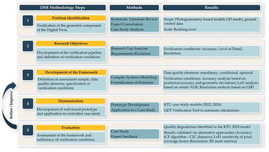
Figure 2.
Research methodology steps.
3.1. Problem Identification and Motivation
The research gap was identified through a systematic literature review, consultation with field experts, and case study analysis, and it is formalized as the lack of a structured, long-term usable approach for verifying the geometric component of Digital Twins, particularly those derived from photogrammetry. This need was also highlighted in a previous review focusing on updating geometric parameters for built assets [32]. Prior research consistently emphasizes the essential requirement for geometric models to accurately represent the state of their physical counterparts [11,12,14,22,25]. Therefore, the verification process must ensure that a newly created model maintains—or, ideally, improves—quality compared to the reference model, thereby making it suitable for subsequent updating. Consequently, a reliable geometric verification approach is critical for twinning and updating processes.
3.2. Research Objectives and Requirements
To develop a verification framework for GDTs, the following research objectives were established:
- RO1: Define the key data quality elements for GDT verification that are both measurable and adaptable to different geometric representations.
- RO2: Develop a verification pipeline, grounded in data quality elements, to produce results indicating either improvement or decline in model quality.
- RO3: Establish conditions to determine whether a model’s quality is maintained, improved, or degraded.
3.3. Design and Development of the Framework
The framework was developed through a multi-step theoretical process as follows:
- Sampling theory was applied to define the scope of data for assessment. The Digital Twins may contain various types of geometric representations, as well as both structured and unstructured data [22]. For unstructured data (e.g., 3D meshes, DSMs), the model scale was used to determine the sample. For structured data (e.g., classified point clouds, segmented models), feature-based sampling can be applied.
- ISO 19157-1:2023 was used as the basis for defining data quality elements, which were further refined to accommodate both structured and unstructured data types, as supported by [33,34,35]. To ensure case specificity, the elements were categorized as mandatory, conditional, or optional. Each data quality element was linked to measurable metrics and organized into three categories: error/correctness indicator, error/correctness rate, and error/correctness count.
- The relationship between model resolution and achievable LoD was formalized by drawing on the LoD definition from [31]. This formalization, coupled with model resolution verification based on GSD, provides a basis for assessing the degree of model simplification that occurs after data processing and model generation.
- Three verification conditions were established based on [15,35] to evaluate model accuracy, resolution, and LoD. These conditions function as decision rules for identifying whether a model’s quality is maintained, improved, or degraded.
3.4. Demonstration of the Framework
To demonstrate the framework’s usability, a prototype web-based tool was developed in Python 3.12.2 to automate calculations and generate a verification score [36]. The GDT Verification Tool compares two geometric models, G(0) (reference) and G(t) (new), applying the three verification conditions (accuracy, resolution, and LoD) to assess the new model’s suitability for replacing the previous version. The developed tool was then used to evaluate case study models and compare the quality of models from different epochs (2022 and 2024) (Supplementary Materials).
3.5. Evaluation of the Framework
The framework was evaluated through its application to a case study, confirming its feasibility in real-world scenarios and the sufficiency of the defined data quality elements. The obtained results were additionally verified using alternative approaches. For accuracy verification, the models were registered using the Iterative Closest Point algorithm, followed by RANSAC segmentation and calculation of cloud-to-cloud (C2C) distances for several planar walls. For LoD assessment, a sensitivity analysis was conducted across a range of pixel coverage factors. For resolution verification, 3D mesh parameters (the number of triangles, average triangle area, mesh surface area, and volume) were calculated to assess differences between models that may indicate simplification.
4. Framework for Verification Geometric Digital Twins
The initial step in verifying a GDT is the setup of the reference model, G(0), as shown in Figure 3. This process involves three mandatory steps: defining the verification sample, specifying data acquisition parameters, and selecting data quality elements. Each of these steps informs the model verification process and the final verification score.
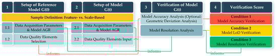
Figure 3.
Verification process of a Geometric Digital Twin.
The representative sample (“Sample Definition”) must be consistently determined for both the reference model, G(0), and the subsequent model, G(t), either based on scale or specific features. However, a feature-based approach is not feasible for geometric models lacking object segmentation and classification. In such cases, like the presented case study, a scale-based sampling method must be applied. To minimize noise and potential outliers caused by obstructions or temporary objects, the case study sample was scale-based and limited to a single building.
Since the models were created under a different complex of conditions that affects the measured accuracy, data acquisition parameters are considered separately for each model. These parameters include camera specifications (focal length, sensor width, and image width) and approximate flight height. This information is then used to calculate the theoretically achievable GSD and compare it with the model’s actual resolution.
The data quality elements, which serve as quantifiable verification metrics, depend on the sample type and must be consistently applied to both models. Accuracy is the only mandatory data quality element, enabling the initial assessment of overall model quality. Conditional elements, such as Commission, Omission, and Temporal Quality, primarily focus on structured models, allowing for the assessment of redundancy, missing data, or object misclassification. Optional data quality elements mainly address data schema compliance, particularly when specified in project requirements. The list of data quality elements for model verification is provided in Table 4. For the case study presented in the paper, Accuracy and LoD compliance were selected as the main data quality measures for assessment.
Table 4.
Data quality elements for Geometric Digital Twin verification.
The setup of both models, including the selection of data quality elements, their corresponding values, and the data acquisition parameters, informs the analysis of each model’s positional accuracy and resolution. This analysis is subsequently used to calculate the verification score. If all three verification conditions (model accuracy, model LoD, and model resolution) are met, it indicates that the new model, G(t), outperforms the reference model, G(0), and is suitable for model updating.
4.1. Model Accuracy Analysis
The model accuracy analysis is based on the positional absolute accuracy (Aabs) and positional relative accuracy (Arel). To assess the consistency of model accuracy over time, the difference between these measures is evaluated as
where RMSREG(t) is Root Mean Square Reprojection Error for model G(t); RMSREG(0) is Root Mean Square Reprojection Error for model G(0); RMSE_GCPG(t) is Root Mean Square Error of Ground Control Points in model G(t); and RMSE_GCPG(0) is Root Mean Square Error of Ground Control Points in model G(0).
If two different GCP networks were used to georeference models G(0) and G(t), then RMSE_GCPG(0) and RMSE_GCPG(t) are calculated separately according to the equations in Table 5.
Table 5.
Calculation of positional accuracy of GCPs.
Condition 1 (Model Accuracy Verification) is met if
- Dacc < δD—the accuracy of model G(t) is consistent with reference model G(0),
- Dacc ≥ δD—the accuracy is inconsistent, indicating degradation in model G(t).
The threshold, δD, can be determined empirically, from the mean and standard deviation of Dacc across multiple geometry update cycles, or normatively, according to project-specific or regulatory requirements. In the case study presented in this paper, ASPRS Positional Accuracy Standards for Digital Geospatial Data, Annex B, was used to establish the threshold, δD [37].
Geometric Deviation Analysis
Geometric deviation analysis is performed based on model alignment. In the presented case study, CloudCompare was used to align the models and calculate deviations. This process helps distinguish true geometric changes from noise or processing artifacts and to identify any positional shift between the models. To identify significant deviations, a positional threshold, δpos, is applied:
where μ is the mean deviation, and σ is the standard deviation.
By the empirical rule (68–95–99.7), ~95% of deviations fall within . If deviations exceed δpos, this indicates misalignment or significant changes in geometry between models.
4.2. Model LoD Verification
Model LoD verification evaluates whether the resolution of model G(t) is sufficient to support the LoD required by the reference model, G(0). While the relationship between a model’s AGR and its LoD is not formally defined, a practical resolution threshold can be established to ensure that LoD-relevant features are reliably represented. To estimate the relationship between the model’s AGR and the minimal feature size required by the LoD, the following algorithm based on “pixel coverage” was used:
- The minimal feature size—representing the smallest features that must be presented in the model—was determined based on Biljecki’s LoD classification, specifically focusing on LoDs 2-3 for photogrammetry-based models.
- Minimal feature representation requirement—these features must be represented by more than 1–2 pixels in the source imagery. Features spanning only 1–2 pixels are considered unreliable due to image noise, blur, and reconstruction uncertainty.
- Pixel coverage for minimal features—the number of pixels required to reliably represent a feature of minimal size. A common practical approach is to ensure that a feature is covered by at least 3 to 5 pixels [38,39,40].
- For the purposes of these calculations, an assumption factor of 4 pixels is applied. This means the minimal feature size should span approximately 4 pixels in the imagery to ensure robust feature reconstruction.
- The LoD is then assigned based on the model’s AGR according to the following relation:
Thus, the model’s AGR indicates whether it can reliably represent LoD-relevant features. For example, a model achieving an AGR of 50 mm/px can capture features as small as 0.2 m (assuming a coverage factor of 4 pixels), making it sufficient for LoD 3.3 modeling. Table 6 provides the necessary model AGR values for LoDs 2.0–3.3, based on the defined minimal feature sizes and 4-pixel coverage factor.
Table 6.
Model’s AGR values for LoDs 2.0–3.3 based on 4-pixel coverage factor.
Since AGR is an average approximation across the model, additional verification of LoD assignment includes comparing the actual dimensions of features within the model (e.g., roof edges, windows) against real-world measurements, which is expressed as RMSE.
Thereby, Condition 2 (Model LoD Verification) evaluates the assigned LoD based on the AGR value of the new model, G(t), against the reference model, G(0), and is satisfied when the LoD of G(t) is consistent with that of G(0).
4.3. Model Resolution Verification
Model resolution analysis compares the achieved resolution of models G(0) and G(t). The achieved resolution is calculated as the ratio of the theoretical GSDcalc (derived from flight and camera parameters) to the actual AGR obtained after model reconstruction. This ratio quantifies the degree to which the reconstructed model deviates from the theoretical resolution.
where H is the flight height, Sw is the sensor width, f is the focal length, and W is the image width.
The achieved resolution ratio near 100% indicates that the model resolution closely matches the theoretical expectation; a ratio significantly below 100% signals a degraded resolution, meaning the reconstruction is coarser than expected. Condition 3 (Model Resolution Verification) is considered satisfied if model G(t) performs equal to or better than model G(0) regarding achieved resolution.
5. Results
5.1. Case Study Description
The Kaunas University of Technology (KTU) campus serves as the case study for validating the framework. As shown in Figure 4, the architecture of the KTU Digital Twin consists of IoT devices and APIs for real-time data collection, SVD for spatial context, and a deployment platform providing data aggregation and a user interface. The SVD includes panoramic photos, BIM models for individual buildings, CAD and GIS data for underground utilities, and a campus-scale photogrammetry model that acts as the main visualization environment. Since the 3D mesh serves as the primary spatial foundation for campus visualization, the need to maintain and regularly update this model to reflect changes in the physical environment is a practical challenge that must be addressed. A detailed description of the case study is provided in Appendix A and reference [41].
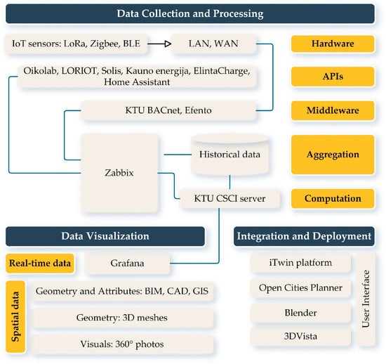
Figure 4.
The architecture of the Digital Twin in the case study.
To validate the framework, two photogrammetry models of the same building from different years—model G(2022) and model G(2024)—were compared. Both data acquisition campaigns occurred while the building was in the Use phase, though part of it was undergoing refurbishment in 2022. Two types of quadcopters were used for image acquisition. In both campaigns, the flights were conducted at an average altitude of approximately 80 m, following an oblique grid pattern with 50% forward overlap and 60% side overlap. GCPs were used for georeferencing and measured with a GNSS RTK rover in the Lithuanian LKS-94 (EPSG:3346) coordinate system. Both datasets were processed using analytical aerotriangulation in Bentley’s iTwin Capture Modeler (formerly Context Capture). The computational setup included an Intel(R) Core(TM) i7-8700 CPU @ 3.20 GHz, 32 GB of RAM, and an NVIDIA Quadro P2000 GPU. Table 7 presents the camera specifications and aerotriangulation results for the G(2022) and G(2024) models.
Table 7.
Camera characteristics and aerotriangulation results for the G(2022) and G(2024) models.
5.2. Model Accuracy Analysis
The model accuracy analysis was performed based on the RMSRE for tie points, which provides the relative positional accuracy, Arel, by aligning the images and creating the 3D structure. The RMSE_GCP provides the absolute positional accuracy, Aabs, by anchoring the model to real-world coordinates. The GCPs ensure that the model is correctly positioned and scaled, correcting for any potential drift or misalignment that may occur when relying solely on tie points.
Two different networks of GCPs were used to georeference the models. The positional accuracy of the GCPs was calculated according to Table 5. The results of the calculations are presented in Table 8 and Table 9 and are used to calculate the accuracy difference between the models (Dacc).
Table 8.
Positional accuracy of GCPs for model G(2022).
Table 9.
Positional accuracy of GCPs for model G(2024).
To assess the consistency of the models’ accuracy over time, the accuracy difference between models, Dacc, was calculated as 0.288. The corresponding threshold, δD, was set at 0.075, based on Table B.5 [32] and the model’s AGR. Since Dacc ≥ δD, this indicates inconsistent accuracy, with the new model, G(2024), demonstrating worse positional performance.
Geometric Deviation Analysis
Models G(2022) and G(2024) were aligned in the CloudCompare software to calculate the geometric deviations using the Cloud-to-Mesh (C2M) distance method, as illustrated in Figure 5. The resulting statistical analysis of the geometric deviation is presented in Table 10.
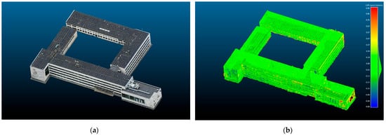
Figure 5.
Range of geometric deviations between G(2022) and G(2024): (a) model view; (b) calculated deviations.
Table 10.
The statistical analysis of geometric deviation between G(2022) and G(2024).
The statistical analysis of the geometric deviations shows an average distance between G(2022) and G(2024) of approximately 0.039 m. Since the mean is positive, model G(2022) tends to lie slightly outside G(2024) on average. A standard deviation of 0.145 m indicates moderate variability in the distances, as shown in Figure 6. The total distance range is 1.500 m, spanning approximately −0.6 m to 0.9 m. This wide range suggests significant deviations at certain points. Visual analysis of the models confirmed that extreme deviations were caused by the vegetation and temporal objects near the building, creating obstructions that affected the model’s reconstruction. Further analysis shows that the majority of the values fall within the range of −0.100 m to 0.150 m. The first quartile (Q1) is 0.025 m, the third quartile (Q3) is 0.774 m, and the resulting interquartile range (IQR) is 0.750 m, representing the middle 50% of the data.
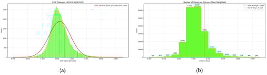
Figure 6.
The statistical analysis of geometric deviation between G(2022) and G(2024): (a) mean and standard deviation; (b) number of geometric deviations per distance class.
To filter out noise and identify significant deviations or misalignment, a threshold, δpos, was calculated as 0.331 m. For the geometric deviations, 96.40% of the values fall below δpos, indicating a high degree of alignment between Models G(2022) and G(2024).
5.3. Model LoD Verification
Condition 2 is validated using the actual AGR values obtained after model reconstruction and the assigned LoD, as defined in Table 6. The assigned LoD is further verified by calculating the RMSE of feature dimensions in the models compared to real-world measurements. Specifically, window dimensions were used as a reference to assess each model’s ability to preserve geometric details.
Based on their AGR values, 20.764 mm/px for G(2022) and 23.242 mm/px for G(2024), both models qualify for LoD 3.3. To confirm this assignment, the dimensions of 14 windows were measured on-site using a Leica Disto D2 laser distance meter, which has a measurement accuracy of ±1.5 mm/m. These measurements were then compared against the corresponding model values at each floor level.
As shown in Table 11, the RMSE increases toward the lower floors, indicating reduced resolution at these levels. This effect is attributed to the flight pattern during data acquisition, which resulted in lower-quality imagery for the building’s lower sections. Furthermore, G(2022) demonstrates generally higher accuracy than G(2024), with an RMSE of 0.15 m compared to 0.21 m, suggesting that geometric features are captured in greater detail in the earlier model.
Table 11.
RMSE of window dimension deviations per floor.
5.4. Model Resolution Verification
Condition 3 is validated by comparing the model’s AGR values with the theoretical GSDcalc, derived from flight and camera parameters. The ratio of AGR to GSDcalc expresses the extent to which the model resolution approaches the theoretical maximum. For model G(2022), the achieved resolution is 89.45%, indicating that the reconstructed model closely reflects the expected resolution. In contrast, model G(2024) achieves only 58.34%, demonstrating reduced performance and a higher degree of resolution loss.
Framework validation results for models G(2022) and G(2024) are presented in Table 12. The comparison indicates that G(2022) outperforms G(2024) across all framework conditions except geometric alignment, where both models show a high degree of consistency. Specifically, model G(2024) demonstrates lower positional accuracy, higher feature RMSE, and a significant loss of resolution.
Table 12.
Framework validation results for models G(2022) and G(2024).
While visual inspection of models can provide an initial impression of quality and help identify major discrepancies, it does not capture subtle yet important differences. The quantitative metrics applied in the developed framework, therefore, allow for a more precise and objective assessment, particularly when evaluating visually similar models. The framework thus offers a structured approach for assessing the quality of photogrammetry-based models used in Digital Twins. To demonstrate its practical usability, the framework has been deployed as a prototype web application, accessible at [36]. A description of its application to the case study is provided in Appendix B.
6. Discussion
6.1. Assessment of the Framework’s Accuracy Analysis
To confirm the results of Condition 1, both models were first converted into point clouds and resampled to one million points each to ensure computational efficiency. The models were then registered using the Iterative Closest Point (ICP) algorithm, which aligns geometries by minimizing Euclidean point-to-point distances to achieve the best geometric fit between datasets, regardless of their reference systems. The resulting ICP RMSE of 0.398 m suggests a moderate level of initial agreement between G(2022) and G(2024). After registration, both point clouds were segmented using the Random Sample Consensus (RANSAC) algorithm, and four main wall planes were extracted from each model for Cloud-to-Cloud (C2C) distance analysis.
As shown in Table 13, the corresponding wall surfaces are nearly parallel in both models, with mean distances ranging from 0.12 to 0.23 m and relatively low variability (standard deviation 0.07–0.26 m). However, the reverse C2C analysis (using G(2024) as the reference) shows higher dispersion in maximum distances. This indicates that G(2024) aligns less precisely and has lower geometric accuracy. Because this analysis relies solely on local geometric correspondence and does not depend on external ground control data, it serves as an alternative validation approach, confirming the framework’s finding that G(2024) shows lower geometric accuracy compared to G(2022).
Table 13.
Calculation of the C2C distances for segmented walls.
6.2. Assessment of the Framework’s LoD and Resolution Analysis
To assess the sensitivity of LoD assignment, the relationship between LoD and AGR was recalculated for pixel coverage factor values from 3 to 10. The results show that both datasets maintain sufficient AGR to support LoD 3.3 modeling for pixel coverage factors between 3 and 8. When the pixel coverage factor exceeds 9, the AGR of G(2024) drops below the LoD 3.3, remaining suitable only for LoD 3.0 representation.
For an alternative assessment of model resolution, several mesh-based metrics were calculated following the approach by Biljecki et al. [31]: total triangle count, average triangle area, surface area, and enclosed volume, as shown in Table 14. Both models preserve a similar total volume (~80,000 m3), confirming that large-scale geometry remains consistent. However, G(2024) contains substantially fewer triangles (0.42 million vs. 5.43 million) and a significantly larger average triangle area (0.045 m2 vs. 0.004 m2), resulting in a more generalized surface and reduced ability to represent fine architectural details.
Table 14.
Three-dimensional mesh metrics for models G(2022) and G(2024).
6.3. Summary of Verification Results
Both the framework results and their verification through alternative approaches indicate a degradation in the quality of model G(2024). Although both models show a high degree of alignment (96.4% of geometric deviations between models are below the δpos threshold of 0.331 m), model G(2024) demonstrates lower positional accuracy based on ground control data (RMSE of 0.073 m vs. 0.026 m for model G(2022)) and a higher reprojection error for tie points (1.49 px vs. 0.67 px), indicating a less accurate reconstruction. These findings were further confirmed using alternative ICP registration and C2C distance calculations. Even without the influence of ground control data, G(2024) shows greater variability in distances and a wider maximum distance range, confirming its lower accuracy.
In terms of achievable LoD, the analysis showed that LoD compliance is the only condition where both models perform almost equally. While the AGR of both models is sufficient for LoD 3.3 modeling, the analysis of façade window dimensions compared with real-world measurements showed that features are slightly less preserved in model G(2024), with an RMSE of 0.21 m vs. 0.15 m for model G(2022). Since the AGR values are quite similar (23.242 mm/px for G(2024) and 20.764 mm/px for G(2022)), a sensitivity analysis of LoD assignment to different pixel coverage factors showed that the models perform similarly overall, diverging only when the pixel coverage factor exceeds 9 pixels.
Considering the model resolution, G(2024) again falls significantly behind G(2022), despite the use of a more advanced camera during data acquisition. Based on GSD calculations, G(2024) achieved only 58.34% of the theoretical resolution that the camera could provide, compared to 89.45% for model G(2022). Alternative mesh-based metrics of the reconstructed models further show a substantial difference in the number of triangles and their average size, while maintaining similar total volume and surface area. This significant difference in triangle count indicates a coarser reconstruction of G(2024), with greater geometric simplification and fewer preserved details.
In general, several factors explain the weaker performance of G(2024). Despite using more GCPs (18 vs. 7), G(2024) was produced as part of a large-scale campus survey (area = 3.59 km2, 3856 images), whereas G(2022) was captured as a standalone model (area = 0.57 km2, 1108 images). Large-area surveys typically require block adjustments during photogrammetric processing, which distribute residual errors across the entire model, consequently reducing local accuracy and resolution within sub-regions. In contrast, the higher image density, greater overlap, and denser GCP distribution relative to the survey size in G(2022) resulted in more precise georeferencing and higher spatial resolution.
6.4. Limitations and Future Work
The study acknowledges several limitations and outlines potential directions for future research. Regarding Condition 2, the established relationship between LoD and AGR should not be interpreted as definitive; rather, it provides a methodological pipeline to guide their alignment. Future research will focus on exploring the sensitivity of this alignment using data-driven approaches to determine optimal AGR thresholds for various LoDs.
The framework’s validation is also constrained by the characteristics of the case study, where both models were represented as unstructured 3D meshes and verification relied on scale-based sampling. Consequently, not all data quality elements—specifically those relevant for feature-based samples—were applicable. Nevertheless, the full list of data quality elements has been retained to support broader applicability in future projects involving different types of models.
To facilitate scalability from single-building analysis to multi-building assessments, future work will investigate the application of Dempster–Shafer theory (also known as the theory of belief functions or evidence theory). This approach can provide a formal mechanism for assigning belief to three states—perform, do not perform, and unknown—based on aggregated evidence from multiple conditions (accuracy, LoD, and resolution). Additionally, it enables dynamic calibration of deviation thresholds. For instance, the current empirical threshold of 95% may be overly strict when evaluating multiple geometric models of varying quality, and it can be refined through the evidence fusion process within Dempster–Shafer theory.
7. Conclusions
A Digital Twin integrates diverse and heterogeneous data sources, with geometric models playing a central role in providing contextual information. These models not only enable visualization but also support advanced applications such as monitoring, simulation, and prediction. However, maintaining and updating the geometric component of a Digital Twin is often neglected due to the high cost and effort associated with digitizing complex environments. Verifying the quality of geometric models is, therefore, a critical step before deciding whether updates are feasible and necessary.
This paper introduces a framework for the verification of GDT, validated using photogrammetry-based models of a university building. The framework specifies three conditions that must be met to verify a newly created model against a reference, enabling a clear determination of quality improvement or degradation. The validation results demonstrate that the proposed data quality elements and verification procedure are sufficient to detect and quantify differences in visually similar models. Based on the framework’s output, we conclusively showed that the new model, intended to replace the version currently used in the Digital Twin, was insufficient and of low quality compared with its predecessor. In addition, a calculation tool has been developed to support the long-term usability of the framework. Accordingly, in line with the research objectives, the developed framework demonstrates measurable data quality elements, proposes a verification workflow, and defines conditions to detect degradation or improvement in geometric model quality.
Although the proposed approach acknowledges certain limitations, including the lack of verification based on structured data, it nonetheless contributes to the broader discussion on the reliability of geometric models within Digital Twins. It provides practical guidance for both researchers and industry practitioners working with image-based methods to develop and deploy Digital Twins.
Supplementary Materials
The following supporting information can be downloaded at https://github.com/iryosa/gdt_tool.git (accessed on 15 September 2025): Geometric Digital Twin Verification Tool (Python source code with software requirements); User Guide; Usage Example.
Author Contributions
Conceptualization, A.J. and M.I.A.; methodology, I.O. and A.J.; software, I.O., J.B.F. and V.B.; validation, D.P. and M.I.A.; formal analysis, D.P. and A.J.; investigation, I.O.; resources, J.B.F. and V.B.; data curation, I.O.; writing—original draft preparation, I.O.; writing—review and editing, A.J., M.I.A. and D.P.; visualization, I.O.; supervision, A.J. and M.I.A. All authors have read and agreed to the published version of the manuscript.
Funding
This research received no external funding.
Data Availability Statement
The original contributions presented in this study are included in the article. Further inquiries can be directed to the corresponding author.
Acknowledgments
The authors would like to thank all the industry and academic experts who gave us their valuable time and feedback during preparation and manuscript proofreading: David Robertson (Bentley Systems), Paris Fokaides (Frederick University, KTU), Stefan Mordue (Bentley Systems), Kieran Mahon (Smart DCU), Rytis Venčaitis (CSCI, KTU), Noel E. O’Connor (Insight SFI RC, DCU), Caroline McMullan (DCU Business School), Celine Heffernan (Insight SFI RC, DCU), Zeljko Djuretic (Bentley Systems), and Vilma Kriaučiūnaitė-Neklejonovienė (KTU). The authors would also like to thank the anonymous reviewers and the editor for their constructive feedback on improving the manuscript.
Conflicts of Interest
The authors declare no conflicts of interest.
Abbreviations
The following abbreviations are used in this manuscript:
| GDT | Geometric Digital Twin |
| SVD | Spatial and Visual Data |
| UAV | Unmanned Aerial Vehicle |
| LoD | Level of Detail |
| BIM | Building Information Model |
| GSD | Ground Sampling Distance |
| AGR | Average Ground Resolution |
| DSM | Digital Surface Model |
| RMSRE | Root Mean Square Reprojection Error |
| GCPs | Ground Control Points |
| DSR | Design Science Research Methodology |
Appendix A
Monitoring of the university environment is achieved by collecting real-time data from various APIs, which transmit over 2000 readings from installed stationary sensors and smart meters. Additional APIs retrieve environmental data from the open Oikolab repository. The collected data is transmitted via an Oracle server to the Zabbix middleware and analyzed on a local KTU server, with Grafana used for time-series data visualization. For the integration of spatial data, 3DVista and Blender are used. This integration supports several services, including the following:
- Operational carbon footprint—the CO2 footprint of the KTU campus, segmented by energy type and aggregated across buildings, systems, and equipment (Figure A3);
- Solar energy production—hourly monitoring of electricity generated from solar panels (Figure A4);
- EV charging stations—usage statistics of campus EV charging points (Figure A5);
- Underground utilities—2D/3D visualizations of gas, water, sewage, and thermal networks, enriched with semantic data (Figure A6).

Figure A1.
Occupancy monitoring.

Figure A2.
Indoor condition monitoring.

Figure A3.
KTU campus CO2 footprint monitoring.

Figure A4.
Electricity production with solar generation.

Figure A5.
EV charging station statistics.

Figure A6.
Three-dimensional views of underground utilities.
Appendix B
The GDT Verification Tool is a prototype web application designed to compare two geometric models: G(0) (the reference) and G(t) (the new model). The tool applies specifically to photogrammetry-based models and evaluates whether the new model meets three conditions—accuracy, LoD, and resolution—relative to the reference. If all conditions are satisfied, the new model is considered suitable for updating the Digital Twin.
The application is organized into three main tabs: model G(0), model G(t), and Verification Results. Model G(0) tab allows users to input reference model data, including optional information on the scale and life cycle stage. Users can define the verification sample, specify parameters for updating, calculate LoD and GSD, and select relevant data quality elements. All inputs can be saved and downloaded as a CSV file (Figure A7 and Figure A8). The model G(t) tab is used to enter data for the newly generated model. The GSD calculation step is mandatory, and only the data quality elements selected in the model G(0) tab are available for input.
The Verification Results tab provides a comparison of models G(0) and G(t). It displays three key summary sections: (1) the “LoD Calculation Summary” shows AGR, suggested LoD, calculated resolution, and feature RMSE; (2) the “Data Quality Elements Summary” lists all selected elements and their values; (3) the “Decision Model” evaluates whether model G(t) meets verification conditions. Optional features within the tab include geometric deviation statistics for pre-aligned models and a performance comparison based on conditional and optional data quality elements, showing where G(t) outperforms G(0). A color-coded “verification score” provides the final assessment of the new model’s suitability for updating. Results can be downloaded as CSV or JSON files (Figure A9 and Figure A10).
The prototype application is deployed on Streamlit, an open-source Python framework for interactive web applications, and its code is publicly available on GitHub. For optimal visualization, enabling the Dark theme (Streamlit—Settings) is recommended.

Figure A7.
GDT Verification Tool web interface—model G(0).

Figure A8.
GDT Verification Tool web interface—selected data quality elements.

Figure A9.
GDT Verification Tool web interface—verification Results.

Figure A10.
GDT Verification Tool web interface—verification score.
References
- Sacks, R.; Brilakis, I.; Pikas, E.; Xie, H.S.; Girolami, M. Construction with Digital Twin Information Systems. Data-Cent. Eng. 2020, 1, e14. [Google Scholar] [CrossRef]
- Grieves, M. Digital Twins: Past, Present, and Future. In The Digital Twin; Crespi, N., Drobot, A.T., Minerva, R., Eds.; Springer Nature Switzerland AG: Cham, Switzerland, 2023; pp. 97–125. [Google Scholar] [CrossRef]
- Madni, A.M.; Madni, C.C.; Lucero, S.D. Leveraging Digital Twin Technology in Model-Based Systems Engineering. Systems 2019, 7, 7. [Google Scholar] [CrossRef]
- Evans, S.; Savian, C.; Burns, A.; Cooper, C. Digital Twins for the Built Environment: An Introduction to the Opportunities, Benefits, Challenges and Risks; The Institution of Engineering and Technology (IET): London, UK, 2019; Available online: https://www.theiet.org/impact-society/policy-and-public-affairs/digital-futures-policy/reports-and-papers/digital-twins-for-the-built-environment (accessed on 18 January 2025).
- Agrawal, A.; Thiel, R.; Jain, P.; Singh, V.; Fischer, M. Digital Twin: Where Do Humans Fit In? Autom. Constr. 2023, 148, 104749. [Google Scholar] [CrossRef]
- Fuller, A.; Fan, Z.; Day, C.; Barlow, C. Digital Twin: Enabling Technologies, Challenges and Open Research. IEEE Access 2020, 8, 108952–108971. [Google Scholar] [CrossRef]
- Kim, Y.-W. Digital Twin Maturity Model. In Proceedings of the WEB 3D 2020 Industrial Use Cases Workshop on Digital Twin Visualization, Online, 13 November 2020. [Google Scholar] [CrossRef]
- Autodesk. What Is a Digital Twin? Intelligent Data Models Shape the Built World. Available online: https://www.autodesk.com/design-make/articles/what-is-a-digital-twin (accessed on 17 January 2025).
- Yue, T.; Arcaini, P.; Ali, S. Understanding Digital Twins for Cyber-Physical Systems: A Conceptual Model. In Leveraging Applications of Formal Methods, Verification and Validation, 9th International Symposium on Leveraging Applications of Formal Methods, ISoLA 2020, Proceedings, Part IV; Springer: Cham, Switzerland, 2020; pp. 54–70. [Google Scholar] [CrossRef]
- ISO 30173:2023; Digital Twin—Concepts and Terminology. International Organization for Standardization (ISO): Geneva, Switzerland, 2023.
- Drobnyi, V.; Fathy, Y.; Brilakis, I. Generating Geometric Digital Twins of Buildings: A Review. In Proceedings of the 2022 European Conference on Computing in Construction, Online, 24–26 July 2022. [Google Scholar] [CrossRef]
- Drobnyi, V.; Hu, Z.; Fathy, Y.; Brilakis, I. Construction and Maintenance of Building Geometric Digital Twins: State of the Art Review. Sensors 2023, 23, 4382. [Google Scholar] [CrossRef] [PubMed]
- Drobnyi, V.; Li, S.; Brilakis, I. Connectivity Detection for Automatic Construction of Building Geometric Digital Twins. Autom. Constr. 2024, 159, 105281. [Google Scholar] [CrossRef]
- Hu, Z.; Fathy, Y.; Brilakis, I. Geometry Updating for Digital Twins of Buildings: A Review to Derive a New Geometry-Based Object Class Hierarchy. In Proceedings of the 2022 European Conference on Computing in Construction, Online, 24–26 July 2022. [Google Scholar] [CrossRef]
- Meyer, T.; Brunn, A.; Stilla, U. Geometric BIM Verification of Indoor Construction Sites by Photogrammetric Point Clouds and Evidence Theory. ISPRS J. Photogramm. Remote Sens. 2023, 195, 432–445. [Google Scholar] [CrossRef]
- University of Galway. RealSim Virtual Campus. Available online: https://www.universityofgalway.ie/about-us/press/publications/e-scealaapril2013/realsimvirtualcampus/# (accessed on 14 October 2024).
- Opoku, D.-G.J.; Perera, S.; Osei-Kyei, R.; Rashidi, M.; Bamdad, K.; Famakinwa, T. Digital Twin for Indoor Condition Monitoring in Living Labs: University Library Case Study. Autom. Constr. 2024, 157, 105188. [Google Scholar] [CrossRef]
- Lu, V.Q.; Parlikad, A.K.; Woodall, P.; Ranasinghe, G.D.; Heaton, J.; DeJong, M.J.; Schooling, J.M.; Viggiani, G.M.B. Developing a Dynamic Digital Twin at a Building Level: Using Cambridge Campus as Case Study. In Proceedings of the International Conference on Smart Infrastructure and Construction 2019 (ICSIC), Cambridge, UK, 8–10 July 2019; ICE Publishing: London, UK, 2019. [Google Scholar] [CrossRef]
- Han, X.; Yu, H.; You, W.; Huang, C.; Tan, B.; Zhou, X.; Xiong, N.N. Intelligent Campus System Design Based on Digital Twin. Electronics 2022, 11, 3437. [Google Scholar] [CrossRef]
- University of Birmingham. Virtual Tour. Available online: https://www.birmingham.ac.uk/virtual-tour (accessed on 15 October 2024).
- Georgetown University. Campus Map. Available online: http://map.concept3d.com/?id=999 (accessed on 15 October 2024).
- Lu, R.; Rausch, C.; Bolpagni, M.; Brilakis, I.; Haas, C.T. Geometric Accuracy of Digital Twins for Structural Health Monitoring. In Structural Integrity and Failure; IntechOpen: London, UK, 2020. [Google Scholar] [CrossRef]
- Crampen, D.; Blankenbach, J. LOADt: Towards a Concept of Level of As-Is Detail for Digital Twins of Roads. In Proceedings of the 30th EG-ICE International Conference on Intelligent Computing in Engineering, London, UK, 4–7 July 2023. [Google Scholar]
- Banfi, F. BIM Orientation: Grades of Generation and Information for Different Type of Analysis and Management Process. Int. Arch. Photogramm. Remote Sens. Spat. Inf. Sci. 2017, XLII-2/W5, 57–64. [Google Scholar] [CrossRef]
- Lammini, A.; Pinquié, R.; Foucault, G.; Noël, F. Geometric Coherence of a Digital Twin: A Discussion. In Product Lifecycle Management. PLM in Transition Times: The Place of Humans and Transformative Technologies; Springer Nature Switzerland: Cham, Switzerland, 2023; Volume 667, pp. 227–236. [Google Scholar] [CrossRef]
- Voytenko, S. Matematychna Obrobka Heodezychnykh Vymiriv. Teoriia Pokhybok Vymiriv: Navchalnyi Posibnyk [Mathematical Processing of Geodetic Measurements. Theory of Measurement Errors: Study Guide]; KNUBA: Kyiv, Ukraine, 2003. (In Ukrainian) [Google Scholar]
- ISO 19157:2013; Geographic Information—Data Quality. International Organization for Standardization (ISO): Geneva, Switzerland, 2013.
- Foote, K.E.; Huebner, D.J. More About GIS Error, Accuracy, and Precision; The Geographer’s Craft Project, Department of Geography, The University of Colorado at Boulder: Boulder, CO, USA, 1995; Available online: https://www.e-education.psu.edu/geog469/node/262 (accessed on 20 October 2024).
- Open Geospatial Consortium (OGC). OGC City Geography Markup Language (CityGML) Encoding Standard; Version 2.0.0 (OGC 12-019); Open Geospatial Consortium: Wayland, MA, USA, 2012. [Google Scholar]
- Biljecki, F.; Ledoux, H.; Stoter, J. Redefining the Level of Detail for 3D Models. Available online: https://www.gim-international.com/content/article/redefining-the-level-of-detail-for-3d-models (accessed on 9 October 2024).
- Biljecki, F.; Ledoux, H.; Stoter, J. An Improved LOD Specification for 3D Building Models. Comput. Environ. Urban Syst. 2016, 59, 25–37. [Google Scholar] [CrossRef]
- Osadcha, I.; Jurelionis, A.; Fokaides, P. Geometric Parameter Updating in Digital Twin of Built Assets: A Systematic Literature Review. J. Build. Eng. 2023, 73, 106704. [Google Scholar] [CrossRef]
- ISO 19157-1:2023; Geographic Information—Data Quality. Part 1: General Requirements. ISO: Geneva, Switzerland, 2023.
- Anil, E.B.; Tang, P.; Akinci, B.; Huber, D. Deviation Analysis Method for the Assessment of the Quality of the As-Is Building Information Models Generated from Point Cloud Data. Autom. Constr. 2013, 35, 507–516. [Google Scholar] [CrossRef]
- Tran, H.; Khoshelham, K.; Kealy, A. Geometric Comparison and Quality Evaluation of 3D Models of Indoor Environments. ISPRS J. Photogramm. Remote Sens. 2019, 149, 29–39. [Google Scholar] [CrossRef]
- Osadcha, I. Geometric Digital Twin Verification Tool. Available online: https://github.com/iryosa/gdt_tool (accessed on 11 September 2025).
- American Society for Photogrammetry and Remote Sensing (ASPRS). ASPRS Positional Accuracy Standards for Digital Geospatial Data. Photogramm. Eng. Remote Sens. 2014, 81, A1–A26. [Google Scholar]
- Bentley Systems. iTwin Capture Modeler User Manual; Bentley Systems, Incorporated: Exton, PA, USA, 2024. [Google Scholar]
- Luhmann, T.; Robson, S.; Kyle, S.; Boehm, J. Close-Range Photogrammetry and 3D Imaging; Walter de Gruyter GmbH & Co KG: Berlin, Germany, 2023. [Google Scholar] [CrossRef]
- Han, J.; Zhu, L.; Gao, X.; Hu, Z.; Zhou, L.; Liu, H.; Shen, S. Urban Scene LOD Vectorized Modeling from Photogrammetry Meshes. IEEE Trans. Image Process. 2021, 30, 7458–7471. [Google Scholar] [CrossRef] [PubMed]
- OpenCities Planner. Kaunas City Digital Twin. Available online: https://eu.opencitiesplanner.bentley.com/www_ktu_edu/kaunasdigitalcity-stage1 (accessed on 6 May 2025).
Disclaimer/Publisher’s Note: The statements, opinions and data contained in all publications are solely those of the individual author(s) and contributor(s) and not of MDPI and/or the editor(s). MDPI and/or the editor(s) disclaim responsibility for any injury to people or property resulting from any ideas, methods, instructions or products referred to in the content. |
© 2025 by the authors. Licensee MDPI, Basel, Switzerland. This article is an open access article distributed under the terms and conditions of the Creative Commons Attribution (CC BY) license (https://creativecommons.org/licenses/by/4.0/).