A Study on the Intelligent Estimation Systems for Costing Traffic Engineering and Landscaping Projects
Abstract
1. Introduction
2. An Intelligent Estimation System for the Drawing Budget of Traffic Engineering and Landscaping Projects
2.1. Determine the Main Factors Affecting the Construction Drawing Budget Pricing Unit
2.1.1. Basic Factors Affecting Construction Drawing Budget Pricing Units
2.1.2. Selecting the Main Influencing Factors for Pricing Units
Design and Distribution of Questionnaires
Processing and Preliminary Analysis of Survey Results
Internal Consistency Reliability and Validity Test
2.1.3. Quantifying the Main Influencing Factors of the Pricing Unit
2.2. Constructing a Historical Database for Construction Drawing Budget Pricing Units
2.2.1. Data Collection and Collation
Territorial Adjustments
Time Adjustment
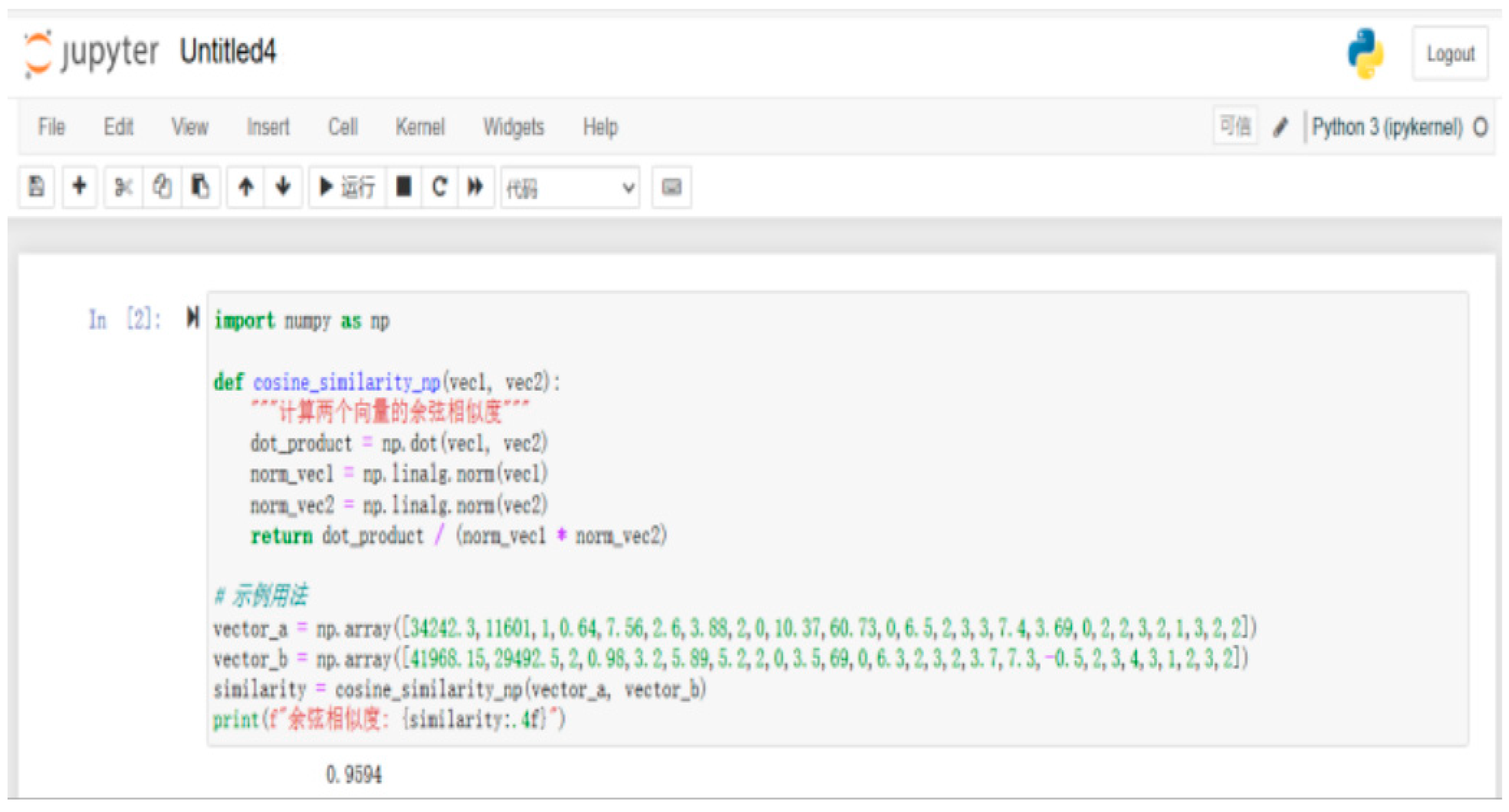
2.2.2. Similar Case Selection Based on the Cosine Similarity Method
2.3. BP Neural Network Method Is Utilized to Estimate the Total Project Cost and Unit Price of Comprehensive Pricing Units Under a Large Amount of Data
- Input layer: The input neurons in the model are the characteristic vectors of the main influencing factors after simplification: the main influencing factors of the construction drawing budget for traffic engineering and landscaping are the input items, and the quantified values of the influencing factors are extracted as the input vector X = (x1, x2, …xn).
- Hidden layer: This study utilizes Kolmogorov’s theorem to calculate the number of hidden layer neurons. The number of hidden layer neurons is 2 times the number of input layer neurons plus 1, alternatively expressed as 2m + 1 (where m signifies the number of input layer neurons).
- Output layer: In conformance to the reviewed literature, the output neuron is the cost per square meter of the target case.
- Parameter design: A three-layer neural network is adopted, including an input layer, a hidden layer, and an output layer. The sigmoid is applied as the activation function, and the stochastic gradient descent algorithm is utilized.
2.4. Intelligent Estimation of Construction Drawing Budgets and a BIM Computer-Aided Model for the Construction of Traffic Engineering and Landscaping Projects
2.4.1. Intelligent Estimation System for the Construction Drawing Budgets of Traffic Engineering and Landscaping Projects
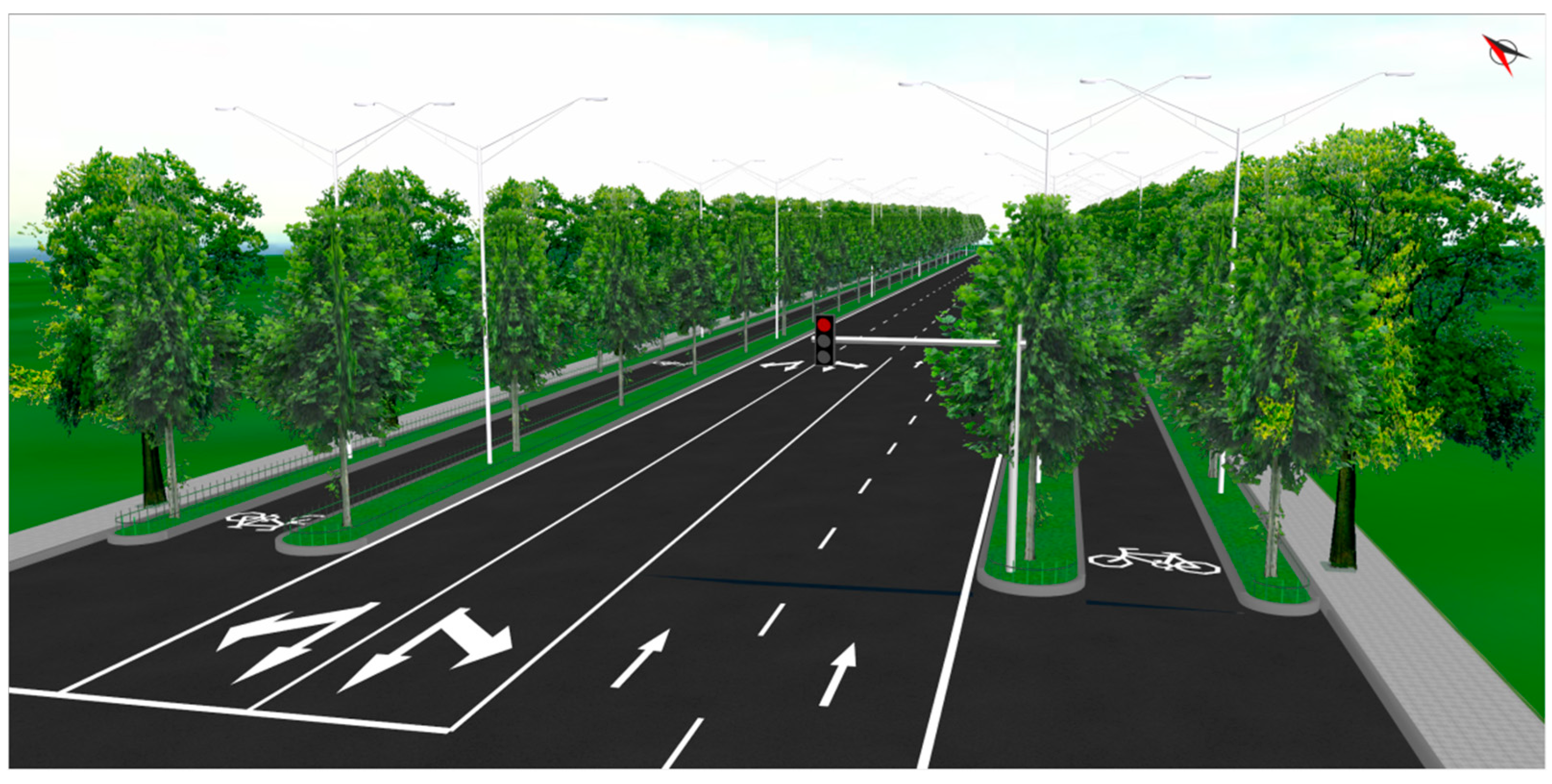
2.4.2. BIM Computer-Aided Visualization Model
- The 3D computer virtual model of the unit project structure is constructed to visualize the overall project structure.
- The 3D computer virtual dynamic model of the construction method and construction procedure is constructed for the dynamic three-dimensional visualization of the construction scheme and construction procedure.
3. Model Implementation
3.1. Target Case-ZGZT Project Overview
3.2. Quantifying Project Characteristics and Calculating Case Similarity for Unit Projects
3.2.1. Quantifying Target Case Characteristics
3.2.2. Case Similarity Calculation
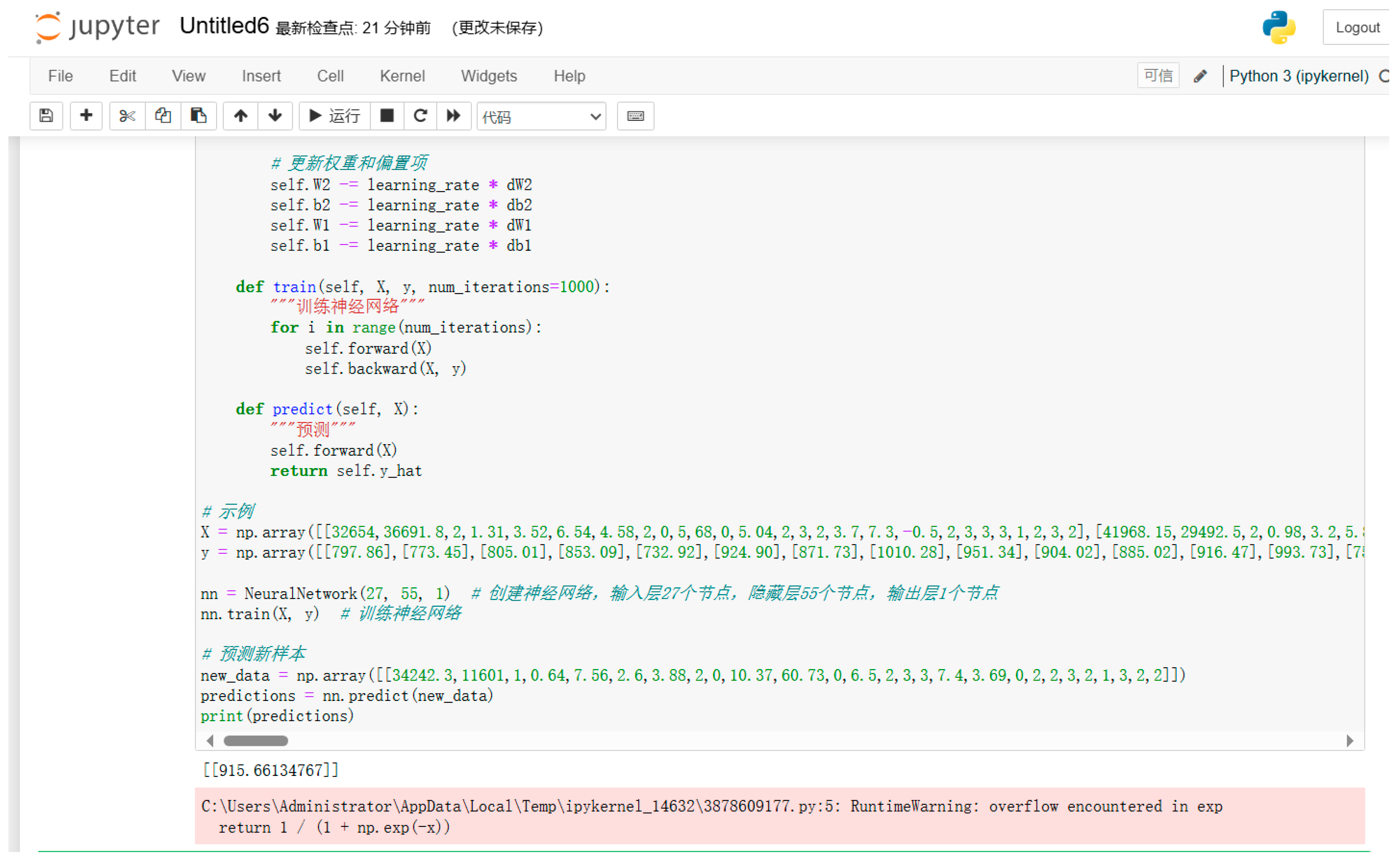
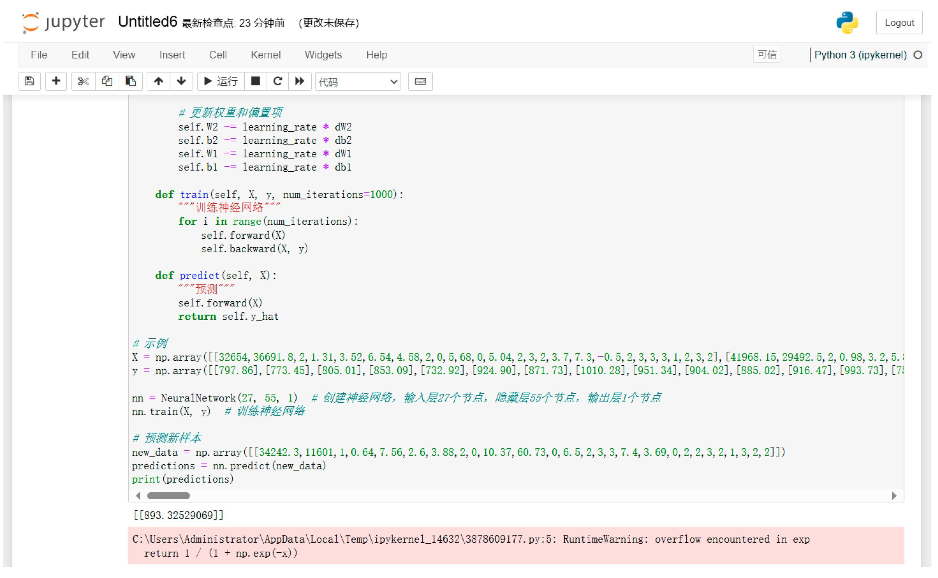
3.3. Comprehensive Unit Price Estimation of Pricing Units Based on the BP Neural Network
- (1)
- The input nodes of the model are determined to be 27, i.e., 27 influencing factors.
- (2)
- The number of hidden layer nodes is determined to be 2 × 27 + 1 = 55.
- (3)
- The model has only one output node, i.e., the project estimate cost per square meter, which signifies the one-time investment consumed for each square meter of land area.
- (4)
- From the 30 case data sets, select 25 cases with a similarity of over 0.85 as training samples, and utilize Case 14 as the test sample. Set the system’s maximum number of iterations to 1000. The main influencing factors, quantified indicators, and cost per square meter for the 25 training samples and 1 test sample are detailed in Table 14.
4. Applying a Computer-Aided 3D and Intelligent Estimation Model for Traffic Engineering and Landscaping Projects
4.1. Constructing a BIM 3D Model
4.2. Developing an Intelligent Estimation System for Construction Drawing Budgets of Traffic Engineering and Landscaping Projects Using PYTHON
5. Conclusions
Author Contributions
Funding
Data Availability Statement
Conflicts of Interest
Appendix A
References
- Elfahham, Y. Estimation and prediction of construction cost index using neural networks, time series, and regression. Alex. Eng. J. 2019, 58, 499–506. [Google Scholar] [CrossRef]
- Wu, X. Research on Cost Control of the Whole Process of Municipal Road Engineering Project Construction. Ph.D. Thesis, Shenyang Jianzhu University, Shenyang, China, 2020. [Google Scholar]
- Wu, X.; Pan, Z. Analysis of Key Points of Cost Control in Each Stage of Municipal Road Engineering Construction. Archit. Budg. 2020, 27–30. [Google Scholar]
- Qiu, Y. Research on the Application of Construction Cost Control in Road Projects. Ph.D. Thesis, Chang’an University, Xi’an, China, 2019. [Google Scholar]
- Wang, H. Research on Cost Control in the Construction Stage of Municipal Road Engineering. Ph.D. Thesis, Anhui University of Finance and Economics, Hefei, China, 2019. [Google Scholar]
- Zhang, H. Research on the Application of BIM Technology in Municipal Infrastructure Projects. Ph.D. Thesis, Beijing University of Civil Engineering and Architecture, Beijing, China, 2018. [Google Scholar]
- Wu, J. Research on Intelligent Estimation Method of Municipal Road Engineering Investment Based on Data Mining. Sci. Technol. Inf. 2025, 23, 159–161. [Google Scholar] [CrossRef]
- Jiang, M.; Yan, M.; Yan, P.; Huang, C.; Tan, S. Factors Influencing Investment Estimation at the Feasibility Study Stage of Municipal Road Projects and Countermeasure Research. Constr. Econ. 2021, 42, 60–64. [Google Scholar] [CrossRef]
- Yang, C. Application of SPSS Project Analysis in Questionnaire Design. High. Corresp. J. (Nat. Sci. Ed.) 2010, 23, 107–109. [Google Scholar]
- Duan, X. Research on the Theory and Method of Comprehensive Investment Control for Government Investment Projects. Ph.D. Thesis, Tianjin University, Tianjin, China, 2007. [Google Scholar]
- Duan, X.; Chen, Y.; Shi, Z.; Huang, K. Research on Intelligent Estimation Methods for Investment in Subway Engineering Construction. J. Railw. Eng. 2021, 38, 109–114. [Google Scholar]

| Classify | Influencing Factor | |
|---|---|---|
| Project features | earth and rock works | Earthwork quantity |
| landscape engineering | Green space arch shape, the proportion of trees, shrubs, bamboo, hedges, open flowers, and lawns | |
| road engineering | Subgrade excavation and shaping, proportion of coarse bituminous concrete pavement, proportion of medium bituminous concrete pavement, proportion of fine bituminous concrete pavement, proportion of cement concrete pavement, proportion of curb area, and road traffic management facilities for engineering | |
| floor space | ||
| erection work | Municipal pipe network project, street lamp project | |
| other | Topography, geology, hydrology, and meteorology | |
| technical management | Construction management level, construction method, degree of intelligence, and ecological civilization construction level | |
| work progress | Change rate of labor and material machine price, change rate of average price of trees, flowers and grass, change rate of average price of asphalt concrete and concrete, environmental protection requirements, quality requirements, and progress requirements | |
| Information | Option | Number of Questionnaires | Proportion |
|---|---|---|---|
| sex | man | 62 | 59.62% |
| woman | 42 | 40.38% | |
| age | 25 and under | 10 | 9.62% |
| 26 to 35 years old | 34 | 32.69% | |
| Age 36–45 | 34 | 32.69% | |
| 46 to 55 years old | 16 | 15.38% | |
| 56 years and over | 10 | 9.62% | |
| highest education | High school and below | 0 | 0.00% |
| junior college | 24 | 23.08% | |
| undergraduate college | 63 | 60.58% | |
| Master’s degree or above | 17 | 16.35% | |
| work unit | design unit | 18 | 17.31% |
| construction organization | 47 | 45.19% | |
| Consulting unit | 26 | 25.00% | |
| Universities/research institutes | 13 | 12.5% | |
| Project experience | 0–3 | 19 | 18.27% |
| Four to six | 37 | 35.58% | |
| 7–9 | 34 | 32.69% | |
| More than 9 | 14 | 13.46% |
| Order Number | Construction Cost Influencing Factors | Mean | Standard Deviation |
|---|---|---|---|
| 1 | Floor space | 3.27 | 0.927 |
| 2 | Earthwork quantity | 3.37 | 0.925 |
| 3 | Green space arch shape | 3.10 | 0.950 |
| 4 | The proportion of trees in the area | 3.56 | 0.923 |
| 5 | Shrub area ratio | 3.53 | 0.945 |
| 6 | The proportion of bamboo area | 2.29 | 0.921 |
| 7 | Green hedge area ratio | 3.45 | 0.974 |
| 8 | The proportion of open field flowers | 3.38 | 0.926 |
| 9 | Lawn area ratio | 2.88 | 0.921 |
| 10 | Subgrade excavation and shaping | 3.00 | 0.975 |
| 11 | Proportion of coarse bituminous concrete pavement | 3.81 | 0.976 |
| 12 | Proportion of medium particle asphalt concrete pavement | 3.82 | 0.983 |
| 13 | Proportion of fine bituminous concrete pavement | 3.88 | 0.952 |
| 14 | Concrete pavement ratio | 3.84 | 0.925 |
| 15 | The proportion of the pavement area | 3.18 | 0.922 |
| 16 | Road traffic management facilities project | 3.49 | 0.935 |
| 17 | Municipal pipe network project | 3.59 | 0.931 |
| 18 | road lamp engineering | 3.21 | 0.931 |
| 19 | Change rate of labor and material machine price | 3.37 | 0.935 |
| 20 | Average rate of change in trees, flowers and grass prices | 3.26 | 0.848 |
| 21 | Average price change rate of asphalt concrete and concrete | 3.52 | 0.892 |
| 22 | Intelligent construction level | 3.52 | 0.975 |
| 23 | Construction management level | 3.38 | 0.948 |
| 24 | The level of ecological civilization construction | 3.27 | 0.916 |
| 25 | Job practice | 3.56 | 0.964 |
| 26 | Environmental protection, quality, and schedule requirements | 2.48 | 0.985 |
| 27 | Landform | 3.43 | 0.993 |
| 28 | Geological conditions | 3.47 | 0.995 |
| 29 | Hydrological conditions | 3.37 | 0.996 |
| 30 | Meteorological conditions | 3.16 | 0.996 |
| Number of Cases | Percentage % | |
|---|---|---|
| valid | 104 | 100.0 |
| get rid of | 0 | 0 |
| amount to | 104 | 100.0 |
| Cronbach’s α | Number of Terms |
|---|---|
| 0.946 | 30 |
| Influencing Factor | Revised Items and Their Correlation to the Total | Cronbach’s α After Deletion |
|---|---|---|
| Floor space | 0.527 | 0.945 |
| Earthwork quantity | 0.755 | 0.942 |
| Green space arch shape | 0.639 | 0.943 |
| The proportion of trees in the area | 0.601 | 0.944 |
| Shrub area ratio | 0.517 | 0.945 |
| The proportion of bamboo area | 0.308 | 0.946 |
| Green hedge area ratio | 0.679 | 0.943 |
| The proportion of open field flowers | 0.560 | 0.944 |
| Lawn area ratio | 0.463 | 0.945 |
| Subgrade excavation and shaping | 0.621 | 0.944 |
| Proportion of coarse bituminous concrete pavement | 0.391 | 0.946 |
| Proportion of medium particle asphalt concrete pavement | 0.383 | 0.946 |
| Proportion of fine bituminous concrete pavement | 0.530 | 0.945 |
| Concrete pavement ratio | 0.406 | 0.946 |
| The proportion of the pavement area | 0.595 | 0.944 |
| Road traffic management facilities project | 0.687 | 0.943 |
| Municipal pipe network project | 0.643 | 0.943 |
| Road lamp engineering | 0.767 | 0.942 |
| Change rate of labor and material machine price | 0.680 | 0.943 |
| Average rate of change in trees, flowers, and grass | 0.609 | 0.944 |
| Average price change rate of asphalt concrete and concrete | 0.558 | 0.944 |
| Intelligent construction level | 0.748 | 0.942 |
| Construction management level | 0.653 | 0.943 |
| The level of ecological civilization construction | 0.675 | 0.943 |
| job practice | 0.638 | 0.943 |
| Environmental quality progress requirements | 0.378 | 0.946 |
| landform | 0.699 | 0.943 |
| Geological conditions | 0.635 | 0.944 |
| Hydrological conditions | 0.673 | 0.943 |
| Meteorological conditions | 0.683 | 0.943 |
| Influencing Factor | ||
|---|---|---|
| KMO price | 0.883 | |
| Bartlett’s sphericity test | Approximate chi-square | 1630.766 |
| Bartlett’s sphericity test | free degree | 435 |
| conspicuousness | 0.000 | |
| Order Number | Influencing Factor | Quantitative Processing | ||||
|---|---|---|---|---|---|---|
| 1 | 2 | 3 | 4 | 5 | ||
| 1 | Floor space | Enter actual data | ||||
| 2 | Earthwork quantity | Enter actual data | ||||
| 3 | Green space arch shape | not have | simple | same as | More complicated | complicated |
| 4 | The proportion of trees in the area | Enter actual data | ||||
| 5 | Shrub area ratio | Enter actual data | ||||
| 6 | The proportion of bamboo area | Enter actual data | ||||
| 7 | Green hedge area ratio | Enter actual data | ||||
| 8 | The proportion of open field flowers | Enter actual data | ||||
| 9 | Lawn area ratio | Enter actual data | ||||
| 10 | Subgrade excavation and shaping | not have | simple | same as | More complicated | complicated |
| 11 | Proportion of coarse bituminous concrete pavement | Enter actual data | ||||
| 12 | Proportion of medium particle asphalt concrete pavement | Enter actual data | ||||
| 13 | Proportion of fine bituminous concrete pavement | Enter actual data | ||||
| 14 | Concrete pavement ratio | Enter actual data | ||||
| 15 | The proportion of the pavement area | Enter actual data | ||||
| 16 | Road traffic management facilities project | not have | simple | same as | More complicated | complicated |
| 17 | Municipal pipe network project | not have | simple | same as | More complicated | complicated |
| 18 | Road lamp engineering | not have | simple | same as | More complicated | complicated |
| 19 | Change rate of labor and material machine price | Enter actual data | ||||
| 20 | Average rate of change in trees, flowers and grass | Enter actual data | ||||
| 21 | Average price change rate of asphalt concrete and concrete | Enter actual data | ||||
| 22 | Intelligent construction level | difference | center | good people | ample | - |
| 23 | Construction management level | difference | center | good people | ample | - |
| 24 | The level of ecological civilization construction | difference | center | good people | ample | - |
| 25 | Job practice | range | secondary | advanced | - | - |
| 26 | Environmental protection, quality, and schedule requirements | same as | higher | tall | - | - |
| 27 | Landform | plain | basin | hills | mountainous region | other |
| 28 | Geological conditions | difference | center | good people | ample | - |
| 29 | Hydrological conditions | difference | center | good people | ample | - |
| 30 | Meteorological conditions | Subtropical Monsoon climate | Temperate continental climate | Monsoon climate of medium latitudes | tropical Monsoon climate | Alpine mountain climate |
| Cosine Similarity | Relativity |
|---|---|
| 0 ≤ < 0.45 | no correlation |
| 0.45 ≤ < 0.85 | correlation |
| 0.85 ≤ < 1 | strong correlation |
| Order Number | Influencing Factor | Signalment |
|---|---|---|
| 1 | Floor space (m2) | 34,242.3 |
| 2 | Earthwork quantity (m3) | 11,601 |
| 3 | Green space arch shape | The project site is flat, and only simplified slope modeling is performed in the green area |
| 4 | The proportion of the area of trees (%) | The area of trees is 219.15 m2, which is 0.64% of the total area |
| 5 | Shrub area ratio (%) | The shrub area is 2588.72 m2, which is 7.56% of the total area |
| 6 | Green hedge area ratio (%) | The hedge area is 890.3 m2, which is 2.6% of the total area |
| 7 | The proportion of open field flowers (%) | The area of flowers is 1328.6 m2, which is 3.88% of the total area |
| 8 | Subgrade excavation and shaping | According to the actual condition of the site where the project is located, simple leveling is performed |
| 9 | Proportion of coarse bituminous concrete pavement (%) | This project does not include a coarse bituminous concrete pavement |
| 10 | The proportion of medium particle asphalt concrete pavement (%) | The area of the medium-sized asphalt concrete pavement is 3550.93 m2, which is 10.37% of the project area |
| 11 | The proportion of fine bituminous concrete pavement (%) | The area of the fine bituminous concrete pavement is 20,795.35 m2, which is 60.73% of the project area |
| 12 | Concrete pavement ratio (%) | This project does not involve cement concrete pavement |
| 13 | The proportion of the curb area (%) | The curb area is 2225.75 m2, which is 6.5% of the project area |
| 14 | Road traffic management facilities project | Equipped with signs and warning posts, this content is quite basic |
| 15 | Municipal pipe network project | Equipped with services including drainage and water supply, the project content is considerably general |
| 16 | Road lamp engineering | Equipped with amenities such as cables and street lamps, the project content is considerably general |
| 17 | Change rate of labor and material machine price (%) | The target case has a price change rate of 7.4% |
| 18 | Average price change rate of trees, flowers and grass (%) | The target case has a price change rate of 3.69% |
| 19 | Average price change rate of asphalt concrete and concrete (%) | The target case has a price change rate of 0% |
| 20 | Intelligent construction level | The command center is applied to control the engineering, monitoring system, and public address system, with a medium level of intelligence |
| 21 | Construction management level | It has a medium level of management by adopting reasonable construction preparation and a rational construction organization plan and construction cost management method |
| 22 | The level of ecological civilization construction | It adopts rational resource utilization and ecological protection methods, and has a satisfactory construction level |
| 23 | Job practice | Adopt a rational construction scheme and construction process, with medium construction methods |
| 24 | Landform | The project is located in Xiongan City, Hebei Province, in the middle of the North China Plain |
| 25 | Geological conditions | The strata are mainly the Quaternary strata of the Cenozoic era |
| 26 | Hydrological conditions | Groundwater mainly comprises pore water and fracture water, and its recharge is mainly from atmospheric precipitation and runoff in the west. |
| 27 | Meteorologic condition | Temperate continental climate |
| Order Number | Influencing Factor | Quantitative Values |
|---|---|---|
| 1 | Floor space (m2) | 34,242.3 |
| 2 | Earthwork quantity (m3) | 11,601 |
| 3 | Green space arch shape | 1 |
| 4 | The proportion of the area of trees (%) | 0.64 |
| 5 | Shrub area ratio (%) | 7.56 |
| 6 | Green hedge area ratio (%) | 2.6 |
| 7 | The proportion of open field flowers (%) | 3.88 |
| 8 | Subgrade excavation and shaping | 2 |
| 9 | Proportion of coarse bituminous concrete pavement (%) | 0 |
| 10 | The proportion of medium particle asphalt concrete pavement (%) | 10.37 |
| 11 | The proportion of fine bituminous concrete pavement (%) | 60.73 |
| 12 | Concrete pavement ratio (%) | 0 |
| 13 | The proportion of the curb area (%) | 6.5 |
| 14 | Road traffic management facilities project | 2 |
| 15 | Municipal pipe network project | 3 |
| 16 | Road lamp engineering | 3 |
| 17 | Change rate of labor and material machine price (%) | 7.4 |
| 18 | Average price change rate of trees, flowers, and grass (%) | 3.69 |
| 19 | Average price change rate of asphalt concrete and concrete (%) | 0 |
| 20 | Intelligent construction level | 2 |
| 21 | Construction management level | 2 |
| 22 | The level of ecological civilization construction | 3 |
| 23 | Job practice | 2 |
| 24 | Landform | 1 |
| 25 | Geological conditions | 3 |
| 26 | Hydrological conditions | 2 |
| 27 | Meteorologic condition | 2 |
| Case | Engineering Feature Quantification Value | ||||||||||||
|---|---|---|---|---|---|---|---|---|---|---|---|---|---|
| X1 | X2 | X3 | X4 | X5 | X6 | X7 | … | X 23 | X 24 | X 25 | X 26 | X 27 | |
| 1 | 32654 | 36,691.8 | 2 | 1.31 | 3.52 | 6.54 | 4.58 | … | 3 | 1 | 2 | 3 | 2 |
| 2 | 41,968.15 | 29,492.5 | 2 | 0.98 | 3.2 | 5.89 | 5.2 | … | 3 | 1 | 2 | 3 | 2 |
| 3 | 20,658 | 11,028.5 | 2 | 1.1 | 3.22 | 6.04 | 4.07 | … | 3 | 1 | 2 | 2 | 2 |
| 4 | 15,171.95 | 16,184.85 | 2 | 1.4 | 3.11 | 6.22 | 4.13 | … | 3 | 1 | 3 | 3 | 2 |
| 5 | 11,067.05 | 4592.92 | 1 | 0.8 | 3.34 | 5.82 | 4.28 | … | 3 | 1 | 2 | 3 | 2 |
| 6 | 52,711.3 | 43,477 | 2 | 0.85 | 7.33 | 4.96 | 3.26 | … | 2 | 3 | 2 | 3 | 2 |
| 7 | 15,394.24 | 10,794.02 | 1 | 1.1 | 6.88 | 5.29 | 4.77 | … | 3 | 1 | 3 | 3 | 2 |
| 8 | 36,325.65 | 15,262 | 2 | 3.78 | 0 | 5.66 | 11.33 | … | 3 | 1 | 2 | 2 | 2 |
| 9 | 21,563.75 | 27,748 | 1 | 3.9 | 2.75 | 4.36 | 2.77 | … | 2 | 1 | 3 | 3 | 2 |
| 10 | 59,463.4 | 10,563 | 1 | 1.25 | 10.66 | 2.74 | 3.41 | … | 3 | 3 | 2 | 3 | 3 |
| 11 | 96,965 | 24,513 | 2 | 1.32 | 3.4 | 8.47 | 4.38 | … | 2 | 1 | 2 | 3 | 2 |
| 12 | 140,951 | 57,429 | 1 | 1.4 | 2.6 | 6.28 | 5.69 | … | 2 | 1 | 3 | 3 | 2 |
| 13 | 35,700.8 | 12,976.4 | 1 | 0.66 | 8.84 | 4.57 | 3.26 | … | 2 | 1 | 3 | 2 | 3 |
| 14 | 17,523.2 | 9734 | 1 | 0.88 | 10.8 | 5.69 | 2.81 | … | 3 | 1 | 3 | 2 | 3 |
| 15 | 25,179.92 | 10,479.1 | 1 | 0.75 | 10.94 | 2.17 | 2.49 | … | 3 | 1 | 3 | 2 | 2 |
| 16 | 29,221 | 1045.5 | 2 | 3.7 | 4.6 | 2.88 | 9.3 | … | 3 | 1 | 3 | 3 | 2 |
| 17 | 17,844.6 | 1729.28 | 2 | 5 | 4.17 | 5.29 | 4.77 | … | 3 | 1 | 3 | 3 | 2 |
| 18 | 11,296 | 1301.65 | 2 | 1.22 | 6.3 | 5.72 | 4.2 | … | 3 | 1 | 3 | 3 | 2 |
| 19 | 10,767 | 1170.1 | 1 | 0.9 | 4.88 | 7.69 | 5.44 | … | 3 | 1 | 3 | 3 | 3 |
| 20 | 21,490 | 27428 | 1 | 0.77 | 7.96 | 5.5 | 4.33 | … | 3 | 1 | 2 | 3 | 2 |
| 21 | 28,945 | 1365.2 | 1 | 1.67 | 4.28 | 8.56 | 4.19 | … | 3 | 1 | 2 | 3 | 2 |
| 22 | 16,382 | 1476.3 | 1 | 1.02 | 3.66 | 7.84 | 6.29 | … | 3 | 1 | 2 | 3 | 2 |
| 23 | 33,760 | 2809.7 | 2 | 0.9 | 9.84 | 4.96 | 2.45 | … | 2 | 3 | 3 | 3 | 3 |
| 24 | 18,673.9 | 23,507.88 | 2 | 1.12 | 5.06 | 8.44 | 3.8 | … | 2 | 1 | 3 | 3 | 2 |
| 25 | 47,306 | 2007.3 | 2 | 0.78 | 9.85 | 4.33 | 3.2 | … | 2 | 1 | 3 | 3 | 2 |
| 26 | 31,074 | 1870.11 | 1 | 0.9 | 5.74 | 8.17 | 4.6 | … | 2 | 1 | 3 | 3 | 2 |
| 27 | 20,769 | 1260.8 | 1 | 1.03 | 3.77 | 7.96 | 5.54 | … | 3 | 1 | 3 | 3 | 2 |
| 28 | 50,386 | 61,470.3 | 2 | 1.17 | 5.13 | 8.88 | 3.29 | … | 2 | 1 | 2 | 3 | 3 |
| 29 | 40,294 | 2409.7 | 1 | 0.77 | 4.96 | 9.4 | 3.85 | … | 3 | 1 | 2 | 2 | 2 |
| 30 | 24,840 | 2067 | 2 | 2.1 | 7.08 | 10.69 | 0 | … | 2 | 3 | 1 | 2 | 3 |
| Order Number | Case Name | Cosine Similarity Value |
|---|---|---|
| 1 | Case 1 | 0.8694 |
| 2 | Case 2 | 0.9594 |
| 3 | Case 3 | 0.9866 |
| 4 | Case 4 | 0.8818 |
| 5 | Case 5 | 0.9978 |
| 6 | Case 6 | 0.9348 |
| 7 | Case 7 | 0.9597 |
| 8 | Case 8 | 0.9975 |
| 9 | Case 9 | 0.8345 |
| 10 | Case 10 | 0.9886 |
| 11 | Case 11 | 0.9969 |
| 12 | Case 12 | 0.9982 |
| 13 | Case 13 | 0.9998 |
| 14 | Case 14 | 0.9838 |
| 15 | Case 15 | 0.9977 |
| 16 | Case 16 | 0.9580 |
| 17 | Case 17 | 0.9737 |
| 18 | Case 18 | 0.9776 |
| 19 | Case 19 | 0.9762 |
| 20 | Case 20 | 0.8367 |
| 21 | Case 21 | 0.9612 |
| 22 | Case 22 | 0.9721 |
| 23 | Case 23 | 0.9705 |
| 24 | Case 24 | 0.8404 |
| 25 | Case 25 | 0.9599 |
| 26 | Case 26 | 0.9647 |
| 27 | Case 27 | 0.9648 |
| 28 | Case 28 | 0.8486 |
| 29 | Case 29 | 0.9646 |
| 30 | Case 30 | 0.9705 |
| Case | X1 | X2 | X3 | X4 | X5 | X6 | X7 | … | X 25 | X 26 | X 27 | The Unit Price per Square Meter Is Yuan/m2 |
|---|---|---|---|---|---|---|---|---|---|---|---|---|
| 1 | 32,654 | 36,691.8 | 2 | 1.31 | 3.52 | 6.54 | 4.58 | … | 2 | 3 | 2 | 797.86 |
| 2 | 41,968.15 | 29,492.5 | 2 | 0.98 | 3.2 | 5.89 | 5.2 | … | 2 | 3 | 2 | 773.45 |
| 3 | 20,658 | 11,028.5 | 2 | 1.1 | 3.22 | 6.04 | 4.07 | … | 2 | 2 | 2 | 805.01 |
| 4 | 15,171.95 | 16,184.85 | 2 | 1.4 | 3.11 | 6.22 | 4.13 | … | 3 | 3 | 2 | 853.09 |
| 5 | 11,067.05 | 4592.92 | 1 | 0.8 | 3.34 | 5.82 | 4.28 | … | 2 | 3 | 2 | 732.92 |
| 6 | 52,711.3 | 43,477 | 2 | 0.85 | 7.33 | 4.96 | 3.26 | … | 2 | 3 | 2 | 924.90 |
| 7 | 15,394.24 | 10,794.02 | 1 | 1.1 | 6.88 | 5.29 | 4.77 | … | 3 | 3 | 2 | 871.73 |
| 8 | 36,325.65 | 15,262 | 2 | 3.78 | 0 | 5.66 | 11.33 | … | 2 | 2 | 2 | 1010.28 |
| 9 | 21,563.75 | 27,748 | 1 | 3.9 | 2.75 | 4.36 | 2.77 | … | 3 | 3 | 2 | 688.57 |
| 10 | 59,463.4 | 10,563 | 1 | 1.25 | 10.66 | 2.74 | 3.41 | … | 2 | 3 | 3 | 951.34 |
| 11 | 96,965 | 24,513 | 2 | 1.32 | 3.4 | 8.47 | 4.38 | … | 2 | 3 | 2 | 904.02 |
| 12 | 140,951 | 57,429 | 1 | 1.4 | 2.6 | 6.28 | 5.69 | … | 3 | 3 | 2 | 885.02 |
| 13 | 35,700.8 | 12,976.4 | 1 | 0.66 | 8.84 | 4.57 | 3.26 | … | 3 | 2 | 3 | 916.47 |
| 14 | 17,523.2 | 9734 | 1 | 0.88 | 10.8 | 5.69 | 2.81 | … | 3 | 2 | 3 | 881.98 |
| 15 | 25,179.92 | 10,479.1 | 1 | 0.75 | 10.94 | 2.17 | 2.49 | … | 3 | 2 | 2 | 993.73 |
| 16 | 29,221 | 1045.5 | 2 | 3.7 | 4.6 | 2.88 | 9.3 | … | 3 | 3 | 2 | 750.92 |
| 17 | 17,844.6 | 1729.28 | 2 | 5 | 4.17 | 5.29 | 4.77 | … | 3 | 3 | 2 | 717.49 |
| 18 | 11,296 | 1301.65 | 2 | 1.22 | 6.3 | 5.72 | 4.2 | … | 3 | 3 | 2 | 672.25 |
| 19 | 10,767 | 1170.1 | 1 | 0.9 | 4.88 | 7.69 | 5.44 | … | 3 | 3 | 3 | 648.43 |
| 20 | 21,490 | 27428 | 1 | 0.77 | 7.96 | 5.5 | 4.33 | … | 2 | 3 | 2 | 729.05 |
| 21 | 28,945 | 1365.2 | 1 | 1.67 | 4.28 | 8.56 | 4.19 | … | 2 | 3 | 2 | 748.17 |
| 22 | 16,382 | 1476.3 | 1 | 1.02 | 3.66 | 7.84 | 6.29 | … | 2 | 3 | 2 | 858.47 |
| 23 | 33,760 | 2809.7 | 2 | 0.9 | 9.84 | 4.96 | 2.45 | … | 3 | 3 | 3 | 908.12 |
| 24 | 18,673.9 | 23,507.88 | 2 | 1.12 | 5.06 | 8.44 | 3.8 | … | 3 | 3 | 2 | 721.27 |
| 25 | 47,306 | 2007.3 | 2 | 0.78 | 9.85 | 4.33 | 3.2 | … | 3 | 3 | 2 | 851.03 |
| 26 | 31,074 | 1870.11 | 1 | 0.9 | 5.74 | 8.17 | 4.6 | … | 3 | 3 | 2 | 791.77 |
| 27 | 20,769 | 1260.8 | 1 | 1.03 | 3.77 | 7.96 | 5.54 | … | 3 | 3 | 2 | 744.67 |
| 28 | 50,386 | 61,470.3 | 2 | 1.17 | 5.13 | 8.88 | 3.29 | … | 2 | 3 | 3 | 924.01 |
| 29 | 40,294 | 2409.7 | 1 | 0.77 | 4.96 | 9.4 | 3.85 | … | 2 | 2 | 2 | 894.17 |
| 30 | 24,840 | 2067 | 2 | 2.1 | 7.08 | 10.69 | 0 | … | 1 | 2 | 3 | 929.95 |
| Sample Number | Estimate the Value of Sample Case 14 (First/m2) | Target Case Estimate (Yuan/m2) | |
|---|---|---|---|
| Estimates | 1 | 846.47 | 900.18 |
| 2 | 850.54 | 902.96 | |
| 3 | 854.82 | 883.08 | |
| 4 | 877.44 | 915.66 | |
| 5 | 870.39 | 893.33 | |
| 6 | 839.86 | 903.92 | |
| 7 | 888.87 | 893.73 | |
| 8 | 870.42 | 890.18 | |
| 9 | 867.35 | 909.67 | |
| Estimates | 10 | 878.83 | 899.43 |
| mean | 864.5 | 899.21 | |
| actual value | 881.98 | 913.16 | |
| Percentage of error | −1.98 | −1.53 | |
| Classical Techniques | 824.71 | 860.53 | |
| Percentage of error | −6.49 | −5.76 | |
Disclaimer/Publisher’s Note: The statements, opinions and data contained in all publications are solely those of the individual author(s) and contributor(s) and not of MDPI and/or the editor(s). MDPI and/or the editor(s) disclaim responsibility for any injury to people or property resulting from any ideas, methods, instructions or products referred to in the content. |
© 2025 by the authors. Licensee MDPI, Basel, Switzerland. This article is an open access article distributed under the terms and conditions of the Creative Commons Attribution (CC BY) license (https://creativecommons.org/licenses/by/4.0/).
Share and Cite
Zhang, D.; Ning, J.; Li, X.; Duan, X. A Study on the Intelligent Estimation Systems for Costing Traffic Engineering and Landscaping Projects. Buildings 2025, 15, 3793. https://doi.org/10.3390/buildings15203793
Zhang D, Ning J, Li X, Duan X. A Study on the Intelligent Estimation Systems for Costing Traffic Engineering and Landscaping Projects. Buildings. 2025; 15(20):3793. https://doi.org/10.3390/buildings15203793
Chicago/Turabian StyleZhang, Dan, Jinxuan Ning, Xing Li, and Xiaochen Duan. 2025. "A Study on the Intelligent Estimation Systems for Costing Traffic Engineering and Landscaping Projects" Buildings 15, no. 20: 3793. https://doi.org/10.3390/buildings15203793
APA StyleZhang, D., Ning, J., Li, X., & Duan, X. (2025). A Study on the Intelligent Estimation Systems for Costing Traffic Engineering and Landscaping Projects. Buildings, 15(20), 3793. https://doi.org/10.3390/buildings15203793


