A ConvLSTM-Based Hybrid Approach Integrating DyT and CBAM(T) for Residential Heating Load Forecast

Abstract

Accurate forecasting of residential heating loads is crucial for guiding heating system control strategies and improving energy efficiency. In recent years, research on heating load forecasting has primarily focused on continuous district heating systems, and it often struggles to cope with the abrupt load fluctuations and irregular on/off schedules encountered in intermittent heating scenarios. To address these challenges, this study proposes a hybrid convolutional long short-term memory (ConvLSTM) model that replaces the conventional batch normalization layer with a Dynamic Tanh (DyT) activation function, enabling dynamic feature scaling and enhancing responsiveness to sudden load spikes. An improved channel–temporal attention mechanism, CBAM(T), is further incorporated to deeply capture the spatiotemporal relationships in multidimensional data and effectively handle the uncertainty of heating start–stop events. Using data from two heating seasons for households in a residential community in Dalian, China, we validate the performance of ConvLSTM-DyT-CBAM(T). The results show that the proposed model achieves the best predictive accuracy and strong generalization, confirming its effectiveness for intermittent heating load forecasting and highlighting its significance for guiding demand-responsive heating control strategies and for energy saving and emissions reduction.

1. Introduction

Accurate forecasting of residential heating load is essential for efficient building energy management. During residential heating, the phenomenon of overheating is widespread and leads to significant energy waste [1]. Accurate heating load forecasting can guide the actual operation of heating systems, improve building energy efficiency, and effectively avoid the energy waste caused by overheating. In practice, residential heating load demand is influenced by multidimensional dynamic factors [2] (e.g., meteorological conditions, floor level, room temperature, and orientation), and heating demand varies substantially across dwellings. These combined influences render residential heating loads markedly nonlinear, nonstationary, and strongly disturbed, which increases the difficulty of load forecasting.

According to the current state of research, heating load forecasting methods can be categorized into physics-based, data-driven, and physics–data hybrid approaches [3,4]. Traditional physics-based models face challenges in quantifying dynamic variations associated with building thermal inertia and multidimensional dynamic factors, especially under intermittent heating scenarios where the load exhibits pronounced abrupt changes. In recent years, data-driven methods have gradually become the mainstream direction for heating load forecasting [5,6]. By mining intrinsic patterns in historical operational data and capturing the effects of multidimensional features, these methods have demonstrated accurate predictive performance in heating load forecasting.

Heating load forecasting, characterized by a significant lag effect, is commonly treated as a time-series prediction task [7]. Data-driven approaches have led to the development of various machine learning and deep learning techniques tailored to such problems. Researchers have improved forecasting performance using both standalone models and hybrid architectures that incorporate attention mechanisms. Machine learning methods such as random forest (RF) [8], support vector regression (SVR) [9], and extreme gradient boosting trees (XGBoost) [10] are particularly effective in modeling nonlinear patterns. Wei et al. proposed an SVR-based supervised learning model optimized using six meta-heuristic algorithms, with the SVR-AEO variant achieving the highest accuracy in predicting residential heating and cooling loads [11]. Ritwik et al. developed a stacked ensemble combining XGBoost [12], decision trees (DT) [13], and RF, which outperformed SVR, k-nearest neighbor (KNN), and artificial neural networks (ANNs) [14]. Lu et al. introduced an AutoML-driven framework that automatically constructs optimal forecasting pipelines [15], demonstrating superior performance over ordinary least squares (OLS) [16], ICA-optimized ANN (ICA-ANN), and SSA-optimized multilayer perceptron (SSA-MLP) [17] on residential datasets. While machine learning models are effective for complex data, they often struggle to capture the spatiotemporal dependencies of heating loads, such as delays in thermal response and meteorological influences. Addressing these limitations is crucial for improving forecast accuracy.

Deep learning models outperform traditional machine learning methods in time-series forecasting by more effectively capturing long-term feature dependencies [18,19]. Architectures such as convolutional neural networks (CNNs) [20], gated recurrent units (GRUs) [21], long short-term memory networks (LSTM) [22], and transformers [23] demonstrate strong capabilities in handling time-series data and mitigating gradient-vanishing problems. Huang et al. introduced a regional heat load forecasting approach using a graph neural network (Ac-GRN), which integrates active deep learning with graph structures to model complex temporal patterns. Evaluated on a Danish district heating dataset for multistep prediction, the method outperformed 11 advanced models, including LSTM, in terms of accuracy, robustness, reliability, and computational efficiency [24]. Zhou et al. developed an air-conditioning heat-load forecasting model based on LSTM optimized via an improved sparrow search algorithm (ISSA-LSTM). By adaptively tuning hyperparameters, the model outperformed RNN, LSTM, and GRU on a custom dataset, significantly enhancing cooling-load prediction accuracy [25]. Zhu et al. proposed an adaptively regulated Kolmogorov–Arnold network (KAN), which adjusts its structure based on input data distribution to better capture local features and nonlinear patterns, maintaining high accuracy even with limited data [26].

Single models often struggle to capture the complex spatiotemporal dynamics of heating load data due to their limited and directional feature extraction capabilities. To address this issue, hybrid models have been developed, leveraging the complementary strengths of multiple architectures to enhance prediction accuracy. Wan et al. introduced the CNN-LSTM-A model to mitigate information loss from long input sequences. The model employs CNN for high-dimensional features and LSTM for capturing temporal dependencies. Experimental results showed that it outperformed conventional LSTM across all metrics [27]. Yan et al. proposed the feature-time transformer encoder-bi-LSTM (FTTrans-E-BL) model, an enhanced transformer-based architecture for short-term load forecasting, to address complex interdependencies in short-term multienergy load forecasting. Validated on real-world data, the model significantly outperformed conventional LSTM in predicting power, heating, and cooling loads [28]. Li et al. developed a convolutional gated recurrent unit (HR-CGRU) model for joint prediction of branch and aggregated district heating loads. It integrates temporal convolutional for feature extraction with a bidirectional GRU enhanced by multihead attention. By leveraging cross-hierarchical temporal dependencies, the model demonstrated superior performance on the combined heat and power load dataset [29].

In recent years, hybrid models have demonstrated good predictive accuracy in heating load forecasting; however, most studies have focused on continuous district heating systems, and research on residential heating load forecasting under intermittent heating scenarios remains relatively scarce, with notable limitations. The primary difference between intermittent and continuous heating is that, in the former, the heating duration, the length of the intermittent interval, and the start–stop times are not fixed, which makes load variations highly abrupt. Under intermittent heating, the switching of operating conditions at start and stop moments can induce short-term spikes in the load, causing severe fluctuations and greatly increasing the difficulty of prediction; even during low-load periods, basic network models may produce physically implausible negative predictions, exposing the shortcomings of existing methods in handling sudden changes in operating conditions. Moreover, although batch normalization, which is widely used in convolutional neural networks, can effectively alleviate gradient explosion and vanishing problems, its tendency to over-smooth time series can also affect the model’s responsiveness to abrupt fluctuations, rendering it insufficiently sensitive to critical variations.

To address the above issues, this study is grounded in practical heating demand and, focusing on the multidimensional dynamic factors of the residential heating process, the operational characteristics of intermittent heating, and the limitations of conventional batch normalization, proposes a hybrid model based on ConvLSTM-DyT-CBAM(T) to effectively tackle the challenges of intermittent heating load forecasting and to enhance forecasting accuracy and stability. The main contributions of this study are as follows:

(1) Fully accounting for the diverse factors affecting heating load forecasting, this study constructs a multisource time-series dataset integrating indoor environmental variables, external weather conditions, and district heating network operating data.

(2) The Dynamic Tanh (DyT) activation function is adopted in place of the conventional batch normalization layer. DyT dynamically adjusts feature scaling according to the data distribution and, via a scaling factor $\alpha$, precisely controls the activation range of the input, avoiding the over-smoothing and compression of extreme values by batch normalization and increasing the model’s responsiveness to abrupt load fluctuations.

(3) The Channel–Spatial Attention Module (CBAM) is improved by introducing a Channel–Temporal Attention Module, CBAM(T), suited to time-series forecasting tasks. By focusing on heating start–stop conditions along the temporal dimension, the module enhances responsiveness to load spikes and convergence, effectively improving the predictive accuracy of intermittent heating loads.

2. Methodology

2.1. Data Preprocessing

The data preprocessing process involves three main steps: cleaning, transformation, and normalization. During cleaning, outliers are corrected, missing values are imputed, and noise is removed. Outlier detection is performed using the interquartile range (IQR) method [30], which identifies values beyond the calculated upper and lower bounds. The method is mathematically defined as follows:

$$\begin{array}{cc}\hfill l_{\mathrm{upper}}& =Q_3+C·IQR\hfill \end{array}$$

(1)

$$\begin{array}{cc}\hfill l_{\mathrm{lower}}& =Q_1-C·IQR\hfill \end{array}$$

(2)

$$\begin{array}{cc}\hfill IQR& =Q_3-Q_1\hfill \end{array}$$

(3)

where $l_{\mathrm{upper}}$ and $l_{\mathrm{lower}}$ denote the upper and lower bounds of the target variable, respectively; $Q_1$ and $Q_3$ represent the first and third quartiles of the target variable data, respectively; C signifies a scaling factor, commonly set to $1.5$ for standard outliers or 3 for extreme cases [31]; and $IQR$ denotes the interquartile range. This study employs $C=3$ to detect extreme outliers.

Given the temporal nature of heating load data, identified outliers are not discarded. Instead, they are corrected using forward–backward mean imputation, consistent with the method applied for missing values. The corresponding mathematical expression is as follows:

$${\widehat{x}}_t={\displaystyle \frac{x_{t-1}+x_{t+1}}{2}}$$

(4)

where ${\widehat{x}}_t$ denotes the missing value at time t, and $x_{t-1}$ and $x_{t+1}$ are the known values at times $t-1$ and $t+1$, respectively. This interpolation method is applied only for short gaps; for large missing intervals, imputation is based on data from similar conditions in the surrounding week.

Following data cleaning, feature construction is performed by generating lagged variables, interaction, and date-based features, which substantially enhance model performance [32]. To reduce computational complexity and address dimensional inconsistencies across data types, Z-score normalization is applied. The corresponding formula is as follows:

$$\tilde{X}={\displaystyle \frac{X-\mu }{\sigma }}$$

(5)

where $\tilde{X}$ represents the normalized data value; X denotes the original data value; $\mu$ refers to the mean of the data; and $\sigma$ signifies the standard deviation.

2.2. eXtreme Gradient Boosting

XGBoost is an ensemble machine learning algorithm based on gradient-boosted decision trees (GBDT), which incrementally fits weak learners to residual errors and aggregates their output to approximate true values [33,34,35]. It incorporates second-order derivatives and regularization to prevent overfitting, enhance convergence, and improve generalization. The model optimizes the objective function in Equation (6) by iteratively refining residuals to improve predictive accuracy.

$${\mathcal{L}}^{\left(t\right)}=\sum _{i=1}^{n}l\left(y_i,{\widehat{y}}_i^{(t-1)}+f_t\left(x_i\right)\right)+\sum _{k=1}^t\Omega \left(f_k\right)$$

(6)

$$\Omega \left(f_k\right)=\gamma T+{\displaystyle \frac{1}{2}}\lambda \sum _{j=1}^T{w}_j^2$$

(7)

where i indexes the ith sample, n denotes the total number of samples, and $l(y_i,{\widehat{y}}_i)$ signifies the loss between the true value $y_i$ and its prediction ${\widehat{y}}_i$. $f_t\left(x_i\right)$ represents the weak learner added at the tth iteration, $x_i$ refers to the feature vector of the ith sample, $\Omega \left(f_k\right)$ denotes the regularization term, T corresponds to the number of tree leaves, $w_j$ represents the weight of the jth leaf, and $\gamma$ and $\lambda$ regulate model complexity and weight penalties to prevent overfitting.

During feature selection, this study employs the weight metric of XGBoost to assess feature importance. Features selected more frequently as split nodes are considered more influential, allowing efficient identification of relevant variables. The corresponding mathematical formulation is as follows:

$${\widehat{I}}_{\mathrm{weight}}\left(j\right)={\displaystyle \frac{I_{\mathrm{weight}}\left(j\right)}{{\sum }_k{I}_{\mathrm{weight}}\left(k\right)}}\times 100\%$$

(8)

where ${\widehat{I}}_{\mathrm{weight}}\left(i\right)$ represents the normalized importance of feature i based on its selection frequency across all split nodes, $I_{\mathrm{weight}}\left(i\right)$ signifies the times feature i is used for splitting, and ${\sum }_k{I}_{\mathrm{weight}}\left(k\right)$ denotes the total number of splits across all features.

2.3. Convolutional Long Short-Term Memory (ConvLSTM)

ConvLSTM combines the strengths of convolutional neural networks (CNNs) and long short-term memory (LSTM) networks [36,37]. While traditional LSTM effectively captures temporal dependencies, it lacks spatial feature extraction capability. ConvLSTM addresses this by replacing fully connected layers with convolutional kernels, enabling joint modeling of spatial and temporal patterns. To accurately represent spatiotemporal dependencies in residential heating load forecasting, this study adopts the ConvLSTM2D architecture for feature extraction.

The key distinction between ConvLSTM and standard LSTM is the replacement of fully connected operations with convolutional operations for updating the memory and hidden states. ConvLSTM consists of four convolution-based components: the input gate ($i_t$), forget gate ($f_t$), cell state ($C_t$), and output gate ($O_t$). The model is defined mathematically as follows:

$$i_t=\sigma \left(W_{xi}\ast X_t+W_{hi}\ast H_{t-1}+W_{ci}\circ C_{t-1}+b_i\right)$$

(9)

where the input gate $i_t$ regulates the information retained in the cell state. It is derived by applying a sigmoid activation to the current input ($X_t$), the previous hidden state ($H_{t-1}$), and the prior cell state ($C_{t-1}$). The forget gate $f_t$ determines the extent to which the previous cell state is retained. It is computed using a sigmoid function applied to the current input, the prior hidden state, and the previous cell state, as follows:

$$f_t=\sigma \left(W_{xf}\ast X_t+W_{hf}\ast H_{t-1}+W_{cf}\circ C_{t-1}+b_f\right)$$

(10)

The candidate cell state ${\tilde{C}}_t$ serves as temporary memory, generated by applying a Tanh function to the current input and previous hidden state. The updated cell state $C_t$ is then computed by combining retained information from the previous state using the forget gate and incorporating the new candidate values, completing the memory update process as follows:

$${\tilde{C}}_t=tanh\left(W_{xc}\ast X_t+W_{hc}\ast H_{t-1}+b_c\right)$$

(11)

$$C_t=f_t\circ C_{t-1}+i_t\circ {\tilde{C}}_t$$

(12)

The output gate $O_t$ regulates the information released from the cell by applying a sigmoid function to the current input, previous hidden state, and updated cell state, determining the final output.

$$O_t=\sigma \left(W_{xo}\ast X_t+W_{ho}\ast H_{t-1}+W_{co}\circ C_t+b_o\right)$$

(13)

The hidden state $H_t$ is obtained by element-wise multiplying the output gate $O_t$ with the cell state passed through a Tanh function:

$$h_t=O_t\circ tanh\left(C_t\right)$$

(14)

In Equations (9)–(14), * indicates convolution, ∘ denotes the Hadamard product, $\sigma$ represents the sigmoid activation function, tanh signifies the hyperbolic tangent function, W and b denote the convolution weights and biases, respectively, and $X_t$, $H_t$, and $C_t$ refer to the input, hidden state, and cell state at time t, respectively. In this study, the data sampling interval is 1 h, and the prediction target is the heating load at the next time step. The input features and window length are determined by a specific feature-selection method and hyperparameter optimization. Each sample window uses measured historical data as the initial condition. The model is trained iteratively according to the aforementioned ConvLSTM equations, and its architecture is shown in Figure 1.

2.4. Dynamic Tanh (DyT)

The hyperbolic tangent (Tanh) function [38] is a widely used nonlinear activation function in neural networks. Its mathematical formulation is given as follows:

$$Tanh\left(x\right)={\displaystyle \frac{e^x-e^{-x}}{e^x+e^{-x}}}$$

(15)

where x is the input value and e denotes the base of the natural logarithm. The Tanh activation function normalizes input values, reducing dimensional inconsistencies from multiscale data. However, under extreme input conditions, it may lead to gradient vanishing during training, thereby hindering convergence and slowing model optimization.

Dynamic Tanh (DyT), introduced by Zhu et al., serves as an alternative to traditional normalization layers by incorporating learnable parameters that modulate the output range of the Tanh function [39]. In this study, DyT is applied to residential heating load forecasting, where it dynamically adjusts to varying data distributions during training. This adaptation mitigates gradient vanishing and improves both the model’s representational ability and training efficiency. The DyT activation function is defined as follows:

$$DyT\left(x\right)=\gamma \ast tanh\left(\alpha x\right)+\beta$$

(16)

where $\alpha$ denotes a scalar parameter that can dynamically scale x at different magnitudes, and $\gamma$ and $\beta$ represent learnable channel-wise vector parameters.

2.5. Channel–Temporal Attention (CBAM(T))

The conventional convolution block attention module (CBAM) comprises channel and spatial attention submodules, which refine spatial feature representations to enhance focus on salient information [40]. However, the spatial component is suboptimal for data-driven regression. To better suit time-series forecasting, this study replaces spatial attention with temporal attention while retaining channel attention [41,42,43]. The architecture is illustrated in Figure 2, and the channel–attention mechanism is defined as follows:

$$\begin{array}{cc}\hfill M_c\left(F\right)& =\sigma \left(MLP\left(AvgPool\right(F\left)\right)+MLP\left(MaxPool\right(F\left)\right)\right)\hfill \\ \hfill & =\sigma \left(W_1\left(W_0{F}_{avg}^c\right)+W_1\left(W_0{F}_{max}^c\right)\right)\hfill \end{array}$$

(17)

where $M_c\left(F\right)$ represents the channel-weight vector; $F\in {\mathbb{R}}^{B\times T\times C}$ denotes the input feature tensor with batch size B, time steps T, and channels C; $\sigma$ signifies the sigmoid activation function; $W_0\in {\mathbb{R}}^{C\times C/r}$ and $W_1\in {\mathbb{R}}^{C/r\times C}$ refer to the shared weights of a two-layer MLP; r corresponds to the channel reduction ratio; and $F_{avg}^c$ and $F_{max}^c$ are the temporal average max-pooled vectors derived from F, respectively.

The temporal attention module is a modified version of the spatial attention mechanism in the conventional CBAM, redesigned to capture temporal dependencies. Its formulation is as follows:

$$\begin{array}{cc}\hfill M_t\left(F\right)& =\sigma \left(f^{1\times k}\left([AvgPool\left(F\right),MaxPool\left(F\right)]\right)\right)\hfill \\ \hfill & =\sigma \left(f^{1\times k}\left([F_{avg}^t,F_{max}^t]\right)\right)\hfill \end{array}$$

(18)

where $M_t\left(F\right)$ represents the temporal weight vector; $f^{1\times k}$ denotes a one-dimensional convolution with kernel length k; $F_{avg}^t$ and $F_{max}^t$ signify the time series derived by applying average and max pooling, respectively, to the input feature F along the channel dimension. The revised temporal attention module applies a convolution across the temporal axis to aggregate critical information from neighboring time steps.

Feature recalibration integrates channel and temporal attention weights through element-wise multiplication with the input, enhancing salient spatiotemporal features while suppressing irrelevant ones. The corresponding formulation is as follows:

$$\tilde{F}=M_c\left(F\right)\otimes F$$

(19)

$$F^{\ast }=M_t\left(F\right)\otimes \tilde{F}$$

(20)

where $\tilde{F}$ signifies the channel-recalibrated feature, $F^{*}$ represents the final output after applying both channel and temporal recalibration, and ⊗ denotes element-wise multiplication.

2.6. Optuna

Optuna is an advanced hyperparameter optimization framework known for its efficiency, flexibility, and ease of use [44]. It achieves rapid optimization through effective sampling and pruning strategies, dynamically defining the search space to identify optimal hyperparameter configurations. Compared with traditional methods such as grid and random search, Optuna significantly reduces both tuning time and the number of required trials.

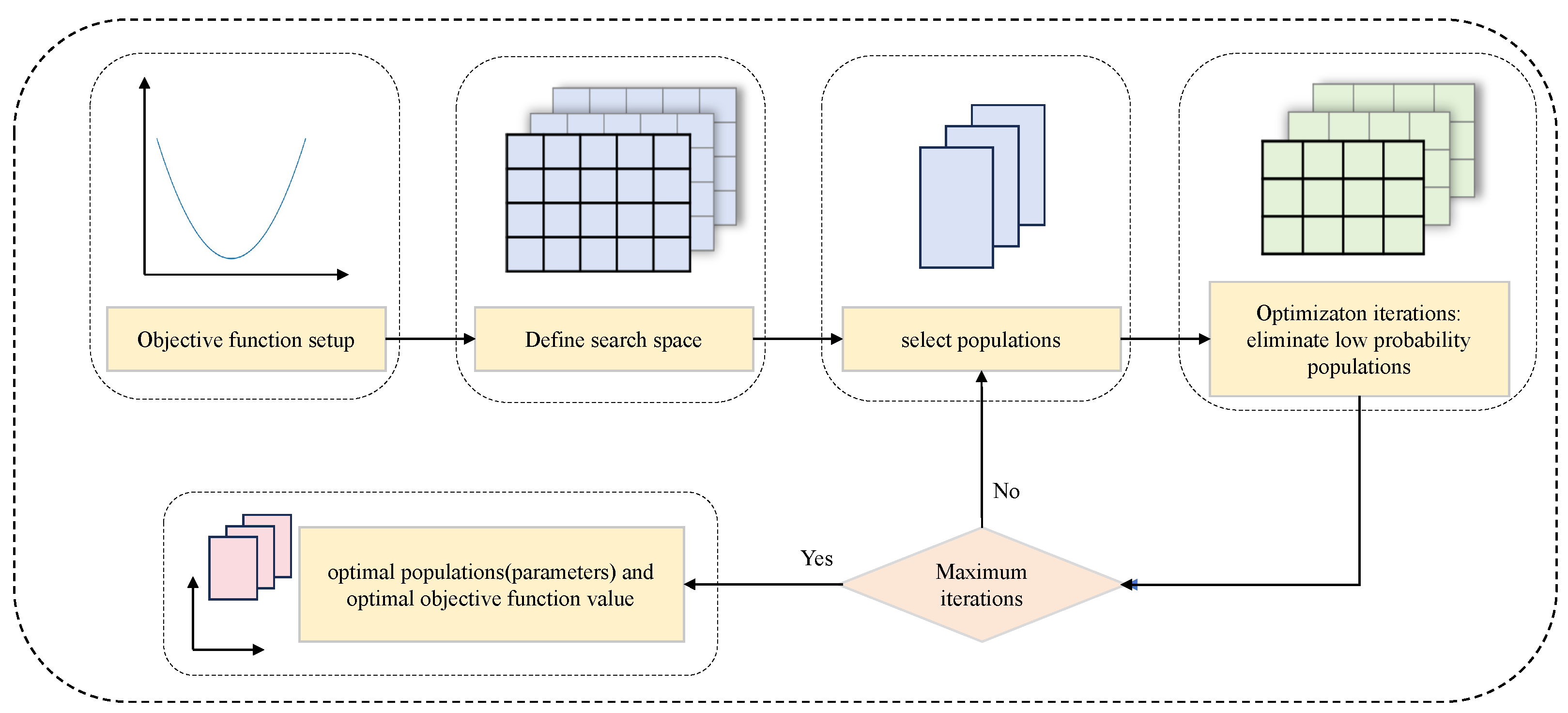
During hyperparameter tuning, Optuna iteratively evaluates parameter combinations within a user-defined objective function and search space, aiming to optimize the objective value. It leverages the tree-structured Parzen estimator (TPE) [45] as its Bayesian optimization core, which models the probability distributions of high- and low-performing configurations to maximize expected improvement. This strategy enables efficient resource allocation toward the most promising hyperparameter sets and parameter combinations. The corresponding mathematical formulation is as follows:

$$E{I}_{y^{*}}\left(x\right)={\displaystyle \frac{l\left(x\right)}{g\left(x\right)}}$$

(21)

where x represents a hyperparameter configuration; y denotes the evaluation metric (MSE) used in this study; $y^{*}$ signifies the performance threshold distinguishing high- and low-quality results; and $l\left(x\right)$ and $g\left(x\right)$ denote the superior and inferior hyperparameter sets, respectively.

During optimization, Optuna utilizes the asynchronous successive halving algorithm (ASHA) to evaluate trial performance. Trials with metrics significantly below the historical median are terminated early to reduce computational cost. The detailed workflow is illustrated in Figure 3.

2.7. ConvLSTM-DyT-CBAM(T)

This study presents a ConvLSTM-DyT-CBAM(T)-based approach for residential heating load forecasting using multiscale time-series data. ConvLSTM serves as the core architecture, integrating the spatial feature extraction capabilities of convolutional neural networks (CNNs) with the temporal sequence modeling of long short-term memory (LSTM) networks to capture spatiotemporal dependencies. The DyT module replaces traditional normalization layers, enabling dynamic feature scaling across varying data distributions and enhancing the model’s capacity to represent nonlinear patterns. In addition, the CBAM-based temporal attention mechanism, CBAM(T) module, introduces temporal attention to improve responsiveness to heating dynamics and load spikes. The model architecture is illustrated in Figure 4.

The multivariate heating-load time series is first preprocessed and transformed into multiscale tensors through down-sampling and feature engineering. A two-layer ConvLSTM network is then employed to jointly extract spatiotemporal features, with the DyT module replacing standard normalization to adaptively scale features across different time scales. A TimeDistributed layer flattens the feature maps while retaining temporal structure, after which the CBAM(T) module applies temporal attention to emphasize relevant information. Finally, globally pooled features are passed through another DyT layer for dynamic scaling and then by fully connected layers to produce a high-accuracy residential heating-load forecast.

2.8. Evaluation Metrics

To assess forecasting accuracy, this study employs three evaluation metrics: mean absolute error (MAE), mean squared error (MSE), and the coefficient of determination ($R^2$), formulated as follows:

$$MAE={\displaystyle \frac{1}{n}}\sum _{t=1}^n\left|y_t-{\widehat{y}}_t\right|$$

(22)

$$MSE={\displaystyle \frac{1}{n}}\sum _{t=1}^n{\left(y_t-{\widehat{y}}_t\right)}^2$$

(23)

$$R^2=1-{\displaystyle \frac{{\sum }_{t=1}^n{(y_t-{\widehat{y}}_t)}^2}{{\sum }_{t=1}^n{(y_t-\overline{y})}^2}}$$

(24)

where n denotes the number of predictions, $y_t$ denotes the actual heating load, ${\widehat{y}}_t$ represents the predicted heating load value, and $\overline{y}$ signifies the mean of the actual heating load.

MAE measures the average magnitude of absolute error; lower values indicate higher accuracy. MSE calculates the mean of squared deviations, penalizing larger errors more heavily; a smaller MSE reflects greater predictive precision. $R^2$ quantifies the proportion of variance in the target variable explained by the model; higher values signify a better fit.

3. Research Design

All experiments were implemented in Python 3.8 and executed on a 64-bit Windows 11 system with an Intel(R) Core (TM) i5-9300H CPU (base frequency 2.40 GHz), NVIDIA GeForce GTX 1650 GPU, and 32 GB of RAM, sourced from Changzhou, China.

3.1. Dataset and Preprocessing

The dataset used in this study was collected from a residential community in Dalian, Liaoning Province. Heat-meter collectors, rooftop weather stations, and indoor thermohygrometers recorded multiple feature parameters simultaneously. The data acquisition period covered the entire 2023 heating season, from 10:00 on 18 November 2023 to 23:00 on 24 March 2024, with hourly intervals, totaling 2822 samples. Of these, 70% were used for training, 10% for validation, and 20% for testing. Data acquisition details are summarized in

Table 1. Multisource heterogeneous data collection information.

Data Category	Feature	Unit	Symbol
Heating Network Parameters	Heating load	kW	HL
	Instantaneous flow rate	m3/h	IF
	Supply water temperature	°C	SWT
	Return water temperature	°C	RWT
Outdoor Meteorological Data	Air temperature	°C	AT
	Air relative humidity	%	AH
	Wind force (Beaufort scale)	Bft	WP
	Wind speed	m/s	WS
	Illuminance	Lux	ILL
Indoor Environmental Parameters	Indoor air temperature	°C	IT
	Indoor relative humidity	%	IH

.

Data collection was occasionally affected by transmission errors and losses due to power outages and signal disruptions. To address this, outliers were corrected and missing values were imputed by the time-series nature of the data (see Section 2.1). Subsequently, uniform normalization was applied to ensure consistency across feature scales.

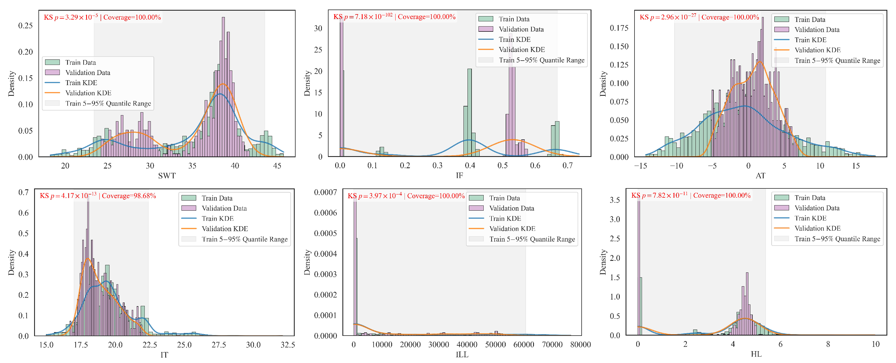
To assess the model’s performance over long time spans and under varying environmental conditions, this study employs cross–heating-season data as an independent validation set. Considering that seasonal changes and operational strategies may induce distribution shift, we diagnose distributional consistency for key variables using the overlap of the 5–95% coverage intervals and the Kolmogorov–Smirnov (KS) test. As shown in

Table 2. KS test results between training and independent validation sets.

Variable	Coverage	KS p-Value
HL	100%	$7.82\times {10}^{-11}$
IF	100%	$7.18\times {10}^{-102}$
SWT	100%	$3.29\times {10}^{-5}$
IT	98.68%	$4.17\times {10}^{-13}$
AT	100%	$2.96\times {10}^{-27}$
ILL	100%	$3.97\times {10}^{-4}$

and Figure 5, the coverage of all variables exceeds 98%, indicating that the validation samples do not fall outside the training empirical domain. However, the KS p-values are very small ($p<0.001$), suggesting significant differences in the data distributions. This result indicates that even when variable ranges are broadly consistent, seasonal alternation and changes in operating strategies can still lead to sample-weight reallocation. On this basis, using cross-season independent validation enables a more objective assessment of the model’s robustness and stability under distributional change.

3.2. Feature Selection

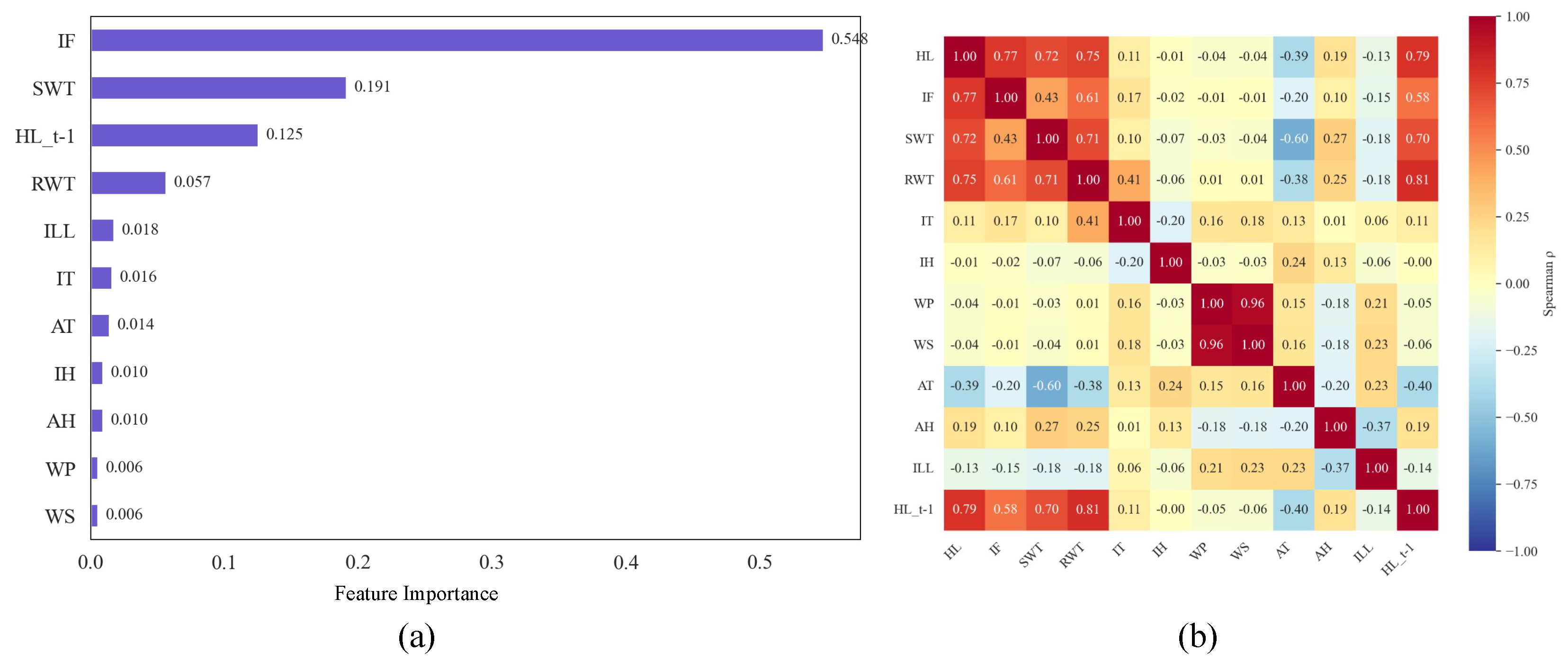
During the feature-selection stage, a multistage screening procedure was employed to optimize the model inputs. First, feature importance was quantified using the XGBoost algorithm, with hyperparameters listed in

Table 3. XGBoost parameter values.

#	Hyperparameter	Values
1	n_estimators	500
2	Learning Rate	0.005
3	Max_depth	5
4	subsample	0.8
5	Min_child_weight	1
6	Reg_$\lambda$	0

and results shown in Figure 6a. Heating-network operating parameters—supply water temperature (SWT), return water temperature (RWT), and instantaneous flow (IF)—exert a dominant influence on forecasting the heating load (HL), which is broadly consistent with thermodynamic principles. However, in practical heating operations, HL is computed from the energy-balance equation combining SWT, RWT, and IF; if all network parameters are included as inputs, the model tends to prioritize supply-side parameters while overlooking dynamic factors such as building thermal inertia, meteorological disturbances, and inter-apartment heat transfer. This leads to degeneration into a basic heat-balance calculator, forfeiting the ability to learn nonlinear dynamics and deviating from the intent of a data-driven model. Accordingly, a critical-parameter truncation strategy is adopted, retaining IF and SWT as representatives of network parameters to reserve more model capacity for learning other potentially relevant factors.

To validate the nonlinear relationships among variables, Spearman correlation analysis was conducted, as shown in Figure 6b. Results indicate a strong positive correlation between IF and HL, a significant negative correlation between air temperature (AT) and HL, and notable associations of indoor temperature (IT) and solar irradiance (ILL) with HL. To account for thermal inertia, the previous heating load $H{L}_{t-1}$ was introduced as a lagged feature, ranking highly in both XGBoost importance and Spearman rank correlation coefficients. Based on multisource heterogeneous data integration, six key features were selected: IF, SWT, $H{L}_{t-1}$, AT, IT, and ILL, to capture the primary influencing dimensions.

3.3. Hyperparameter Optimization Based on Optuna

To ensure equitable hyperparameter tuning, all models in this study were optimized using the Optuna framework, with a unified hyperparameter search space and step sizes. Detailed hyperparameters are provided in

Table 4. Hyperparameter-optimization search space.

#	Hyperparameter	Search Space	Step
1	Units1 or Filters1	[16, 512]	16
2	Units2 or Filters2	[16, 256]	16
3	Num_heads	[2, 8]	2
4	Key_dim	[16, 128]	16
3	Dropout1	[0, 0.5]	0.05
4	Dropout2	[0, 0.5]	0.05
5	Learning rate	[$1\times {10}^{-5}$, $1\times {10}^{-2}$]	$1\times {10}^{-5}$
6	Batch size	{16, 32, 64}	–
7	Time steps	[1, 6]	1
8	CBAM(T) ratio	[4, 16]	4
9	Temporal kernel	[3, 12]	3
10	DyT_alpha1	[0.1, 1.5]	0.1
11	DyT_alpha2	[0.1, 1.5]	0.1

.

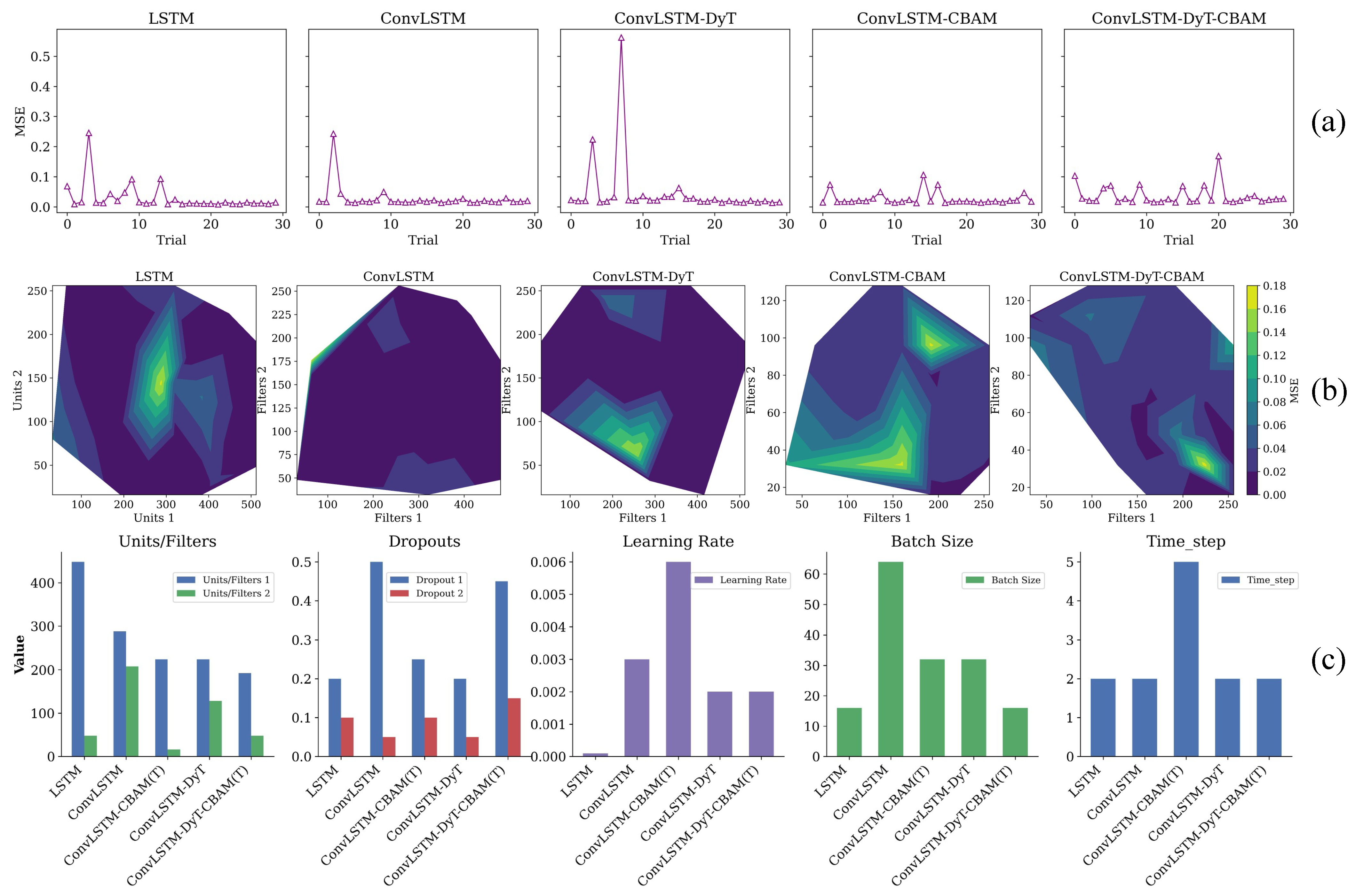
Using the defined hyperparameter search space and time steps, the optimized hyperparameters obtained via Optuna are summarized in

Table 5. Hyperparameter-optimization results across models.

Hyper Parameters	LSTM	CNN -Transformer	KAN	ConvLSTM	ConvLSTM -CBAM(T)	ConvLSTM -DyT	ConvLSTM -DyT -CBAM(T)
Units1/Filters1	448	256	208	288	224	224	192
Units2/Filters2	48	112	208	208	16	128	48
Num_heads	-	4	-	-	-	-	-
Key_dim	-	80	-	-	-	-	-
Dropout1	0.20	0.35	0.05	0.50	0.25	0.20	0.45
Dropout2	0.10	-	0.30	0.05	0.10	0.05	0.15
Learning_rate	0.001	0.002	0.001	0.003	0.007	0.002	0.002
Batch_size	16	16	16	64	32	32	16
Time_step	2	2	3	2	5	2	2
DyT_alpha1	-	-	-	-	-	1.9	0.5
DyT_alpha2	-	-	-	-	-	0.9	0.9
CBAM(T)_ratio	-	-	16	-	-	8	-
Temporal_kernel	-	-	6	-	6	-	6

. Figure 7 presents a comparative analysis of the optimization results. Specifically, Figure 7a shows the MSE convergence trend across models, indicating that all achieved similar optimal values. Figure 7b visualizes the relationship between key model parameters (e.g., number of hidden units, filter size) and MSE using a contour plot, where contour density directly reflects the sensitivity of MSE to parameter changes. Darker colors indicate lower error; sparser contours and more contiguous low-error regions imply reduced sensitivity to hyperparameter perturbations. Figure 7c compares the optimal hyperparameter combinations across models using a histogram, highlighting differences in configuration strategies.

4. Prediction Results and Analysis

4.1. Prediction Results of Residential Heating Load

To verify the effectiveness of the ConvLSTM-DyT-CBAM(T) model, ablation and comparative experiments were conducted, and two advanced models in this field—CNN-Transformer and the adaptive Kolmogorov–Arnold network (KAN)—were selected for comparison. To ensure experimental fairness, all models adopted the same hyperparameter optimization procedure, with the optimal configurations determined via Optuna. The specific hyperparameter settings for each model are provided in Table 5.

As shown in

Table 6. Comparison of prediction results across models.

#	Model	MSE	MAE	R2
1	LSTM	0.090	0.216	0.972
2	CNN-Transformer	0.251	0.403	0.951
3	KAN	0.052	0.147	0.990
4	ConvLSTM	0.065	0.191	0.987
5	ConvLSTM-CBAM(T)	0.060	0.179	0.988
6	ConvLSTM-DyT	0.038	0.135	0.993
7	ConvLSTM-DyT-CBAM(T)	0.017	0.082	0.997

, the evaluation metrics for the different models include MSE, MAE, and R², while Figure 8 provides a visual comparison of these metrics across models. The results indicate that the LSTM model attains MSE, MAE, and R² values of 0.090, 0.216, and 0.972, respectively, revealing certain limitations in capturing the complex dependencies of multidimensional time series. Incorporating convolutional structures, ConvLSTM offers advantages in modeling spatiotemporal dependencies; its MSE, MAE, and R² are 0.065, 0.179, and 0.987, outperforming LSTM. Building on ConvLSTM, integrating the improved attention mechanism CBAM(T) enhances the model’s responsiveness to load fluctuations; relative to ConvLSTM, its MSE and MAE are reduced by 7.69% and 6.28%, and R² increases by 0.1%. In the ConvLSTM–DyT model, replacing the conventional batch normalization layer with the dynamic Tanh activation avoids under-responsiveness to sudden and spiky load variations caused by over-smoothing. Compared to ConvLSTM, MSE and MAE decrease by 41.54% and 29.32%, and R² increases by 0.61%. As a comparison model, CNN–Transformer yields MSE, MAE, and R² of 0.251, 0.403, and 0.951, respectively, representing relatively weaker performance. Although this model often performs well on medium- to long-term forecasting tasks, it is highly data-dependent, and the limited data available for the present short-term heating-load task may have degraded its predictive performance. The KAN model performs strongly, with all metrics surpassing those of the ConvLSTM–CBAM(T) and ConvLSTM–DyT hybrids, achieving MSE, MAE, and R² of 0.052, 0.147, and 0.990, respectively, second only to the best model. The proposed ConvLSTM–DyT–CBAM(T) hybrid, which combines the advantages of temporal–channel attention and Dynamic Tanh, performs best: its MSE, MAE, and R² are 0.017, 0.082, and 0.997, representing reductions of 73.85% and 57.07% in MSE and MAE and an increase of 1.01% in R² relative to ConvLSTM. Even compared with KAN, MSE and MAE are further reduced by 67.31% and 44.22%, and R² increases by 0.71%.

4.2. Analysis of Prediction Results

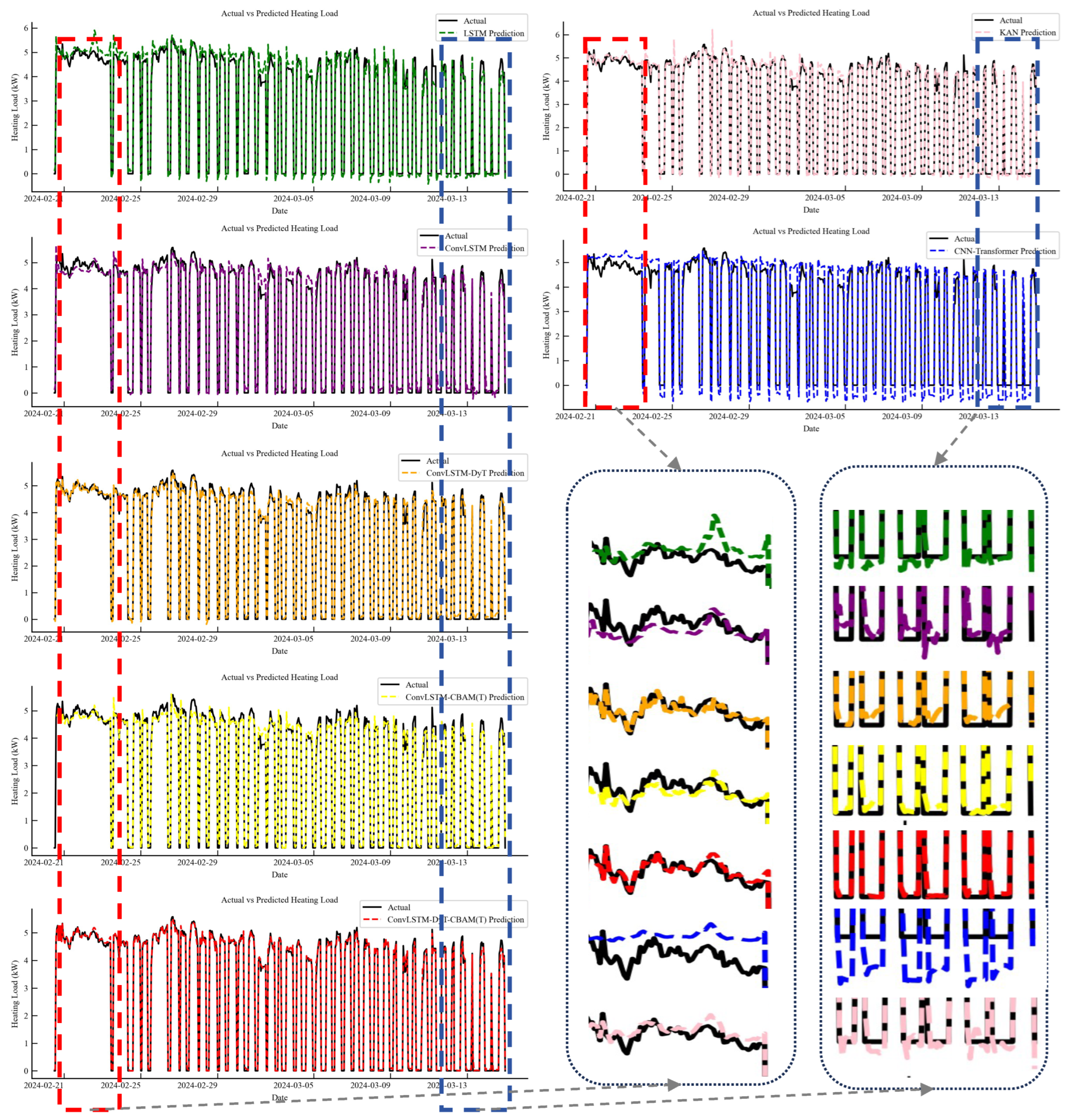
Figure 9 presents a comparison between each model’s predicted heating loads and the ground-truth curve on the test set. The right-hand side provides locally magnified views of peak and valley segments to more clearly examine each model’s grasp of heating start–stop instants and its responsiveness to spike-like load surges. Red and blue dashed boxes denote the regions magnified for peaks and valleys, respectively.

LSTM (green curve) markedly overestimates in peak regions and yields physically implausible negative values in valley regions, primarily because the model’s relatively simple architecture struggles to capture abrupt fluctuations in residential heating loads under intermittent heating. With the introduction of convolutional structure, the ConvLSTM model (purple curve) achieves some improvement in predictive accuracy and is smoother overall; its peak fitting surpasses that of LSTM, yet negative predictions persist in valley regions, indicating limited ability to capture burst features in intermittent heating.

By replacing the conventional normalization layer with the Dynamic Tanh activation, the ConvLSTM-DyT model (orange curve) produces peak-region predictions that largely track the fluctuations of the true curve and essentially eliminate negative values in valleys; however, at the critical transition instants of heating on/off, prediction lag remains, and the curve does not fully and smoothly converge to zero.

Integrating the improved temporal–channel attention mechanism, the ConvLSTM-CBAM(T) model (yellow curve) is slightly inferior to ConvLSTM-DyT in peak-region fitting but superior in valley regions. Around the critical start–stop points, the valley-region predictions also basically converge smoothly to zero, indicating strong responsiveness.

As a comparison model, the CNN–Transformer (blue curve) performs well on medium- to long-term forecasting tasks; however, its global weighting characteristic tends to produce over-smoothing and phase delays for sparse start–stop transients. Consequently, it is difficult for the model to fit the fluctuation pattern in peak regions, and sizable negative-load predictions appear in valley periods. In addition, this model requires a larger amount of data and, thus, fails to fully exploit its advantages under the intermittent-heating scenario studied here. The KAN model (pink curve) can compose basis functions to fit smooth higher-order trends, but it lacks recurrent state and temporal gating to handle regime switching; although it shows good fitting performance at peaks, it still cannot overcome the problem of negative-load predictions in valley regions during heating on/off.

The proposed ConvLSTM-DyT-CBAM(T) model (red curve), combining the strengths of DyT and CBAM(T), performs best overall. It accurately fits the true heating-load curve in both peak and valley regions; in particular, at moments of rapid load change induced by intermittent heating, it responds quickly and precisely captures short-term fluctuation trends, clearly surpassing the other models. This is mainly attributable to the hybrid model’s multimodule complementary advantages. The convolutional recurrence of ConvLSTM preserves phase and amplitude information between adjacent time steps within local spatiotemporal neighborhoods, which confers an advantage in handling the start–stop transients of intermittent heating; DyT dynamically adjusts feature scales, strengthening the model’s ability to capture fine-grained features so that it can capture external information that more closely reflects reality and accurately predict the true behavior of the heating system, while avoiding the over-smoothing of features near zero load that would reduce model sensitivity and lead to negative load predictions. CBAM(T) highlights heating-load–related key variables along the channel dimension and focuses on start–stop windows and spike segments along the temporal dimension, thereby reducing the interference of slowly varying factors with the identification of abrupt changes. Working in concert, these three components effectively address the challenges of uncertain start–stop timing and inaccurate prediction of abrupt load changes in intermittent-heating scenarios, exhibiting excellent adaptability and precision under complex operating conditions.

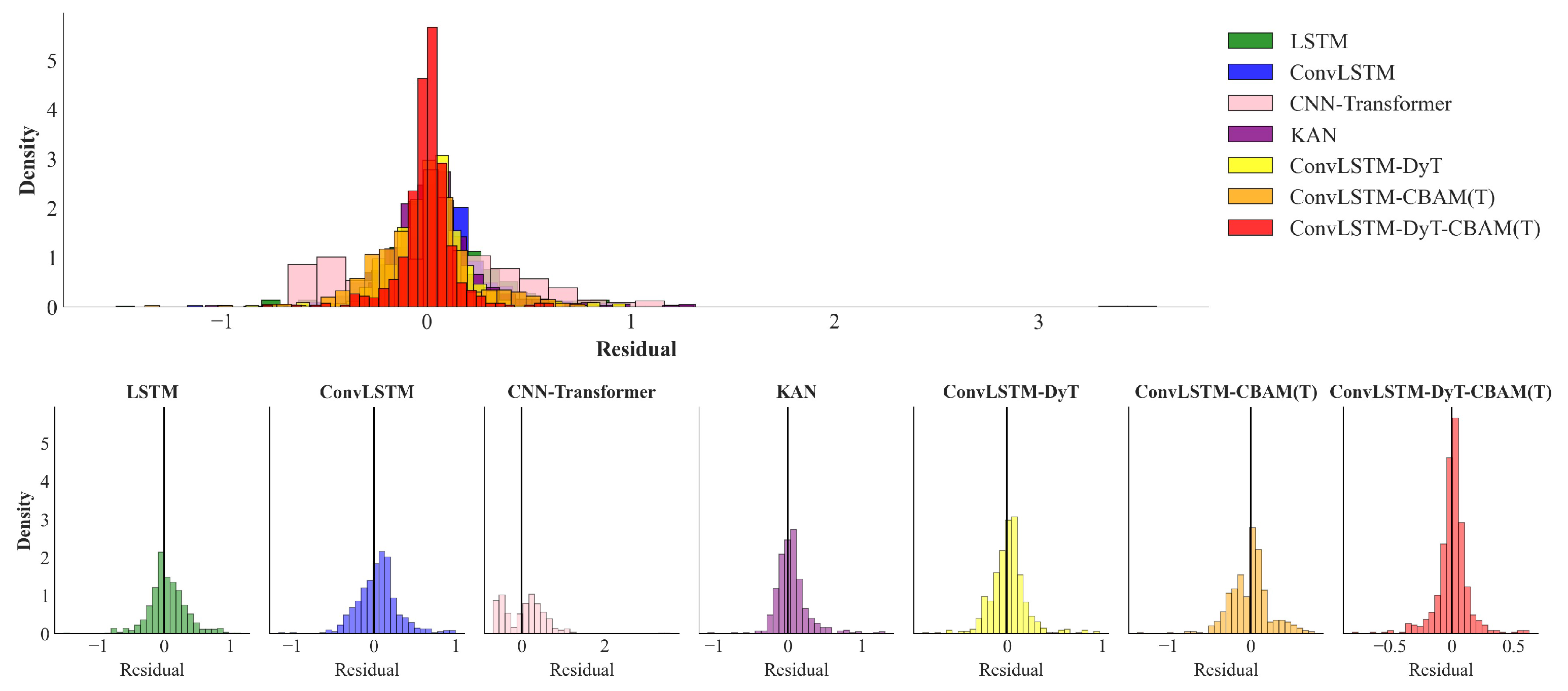
Figure 10 presents the residual distributions of the forecasting models, where the vertical axis denotes residual density and the black line marks zero error. The ConvLSTM-DyT-CBAM(T) model shows the narrowest distribution and highest peak, reflecting minimal prediction error and superior stability compared with other models.

4.3. Analysis of Cross-Season Validation Results

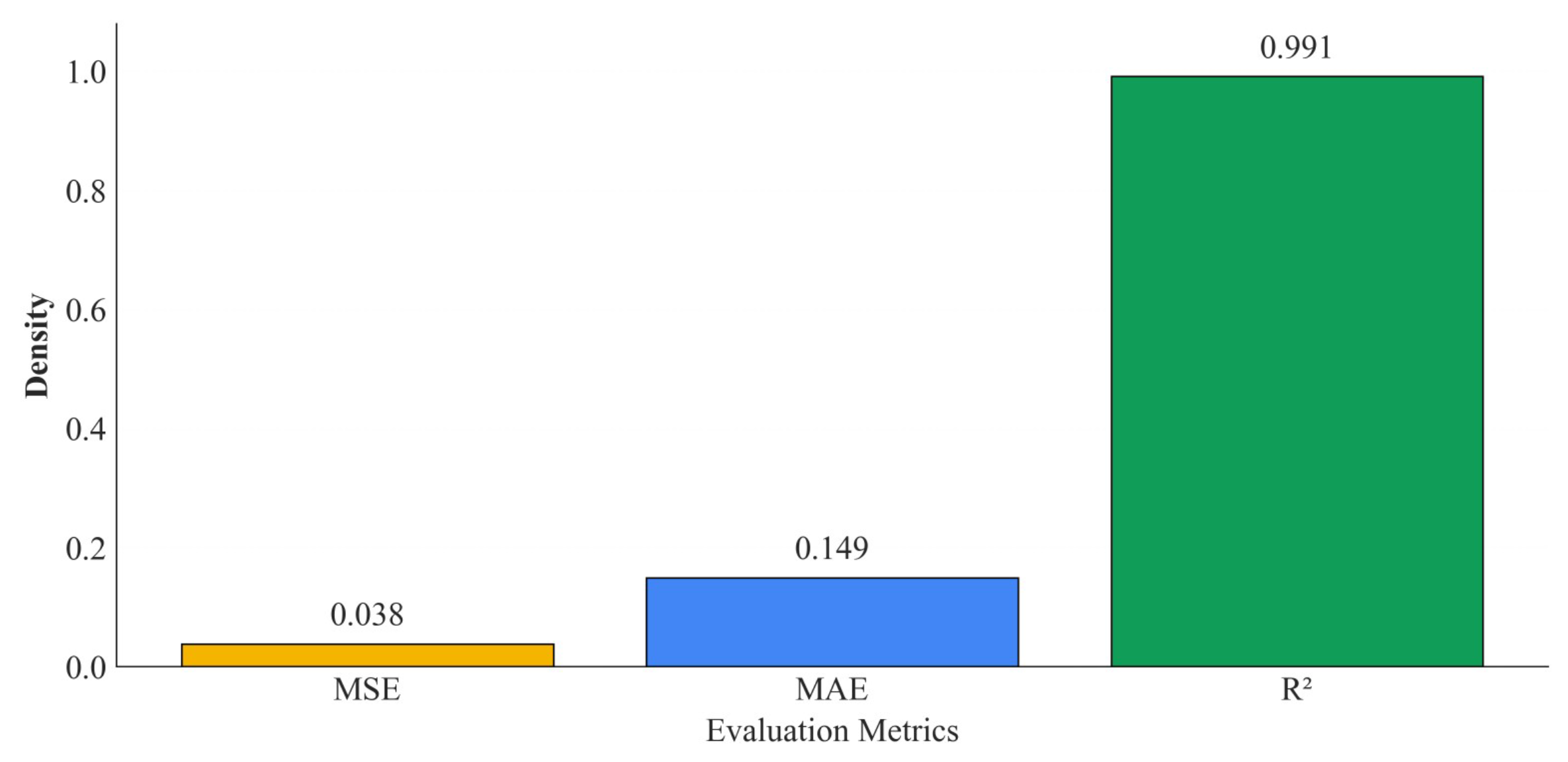
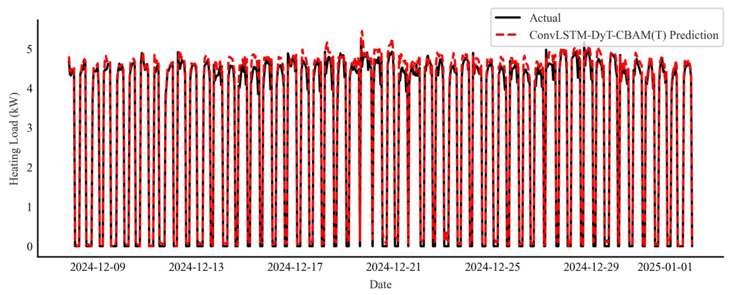
Figure 11 and Figure 12 present the accuracy metrics and the prediction–ground-truth comparison curves of the ConvLSTM-DyT-CBAM(T) model on the independent validation data. The MSE, MAE, and R² are 0.038, 0.149, and 0.991, respectively. Although the overall performance is slightly inferior to that on the test set, it remains at a high level of accuracy. In the comparative curves, the model largely preserves its test-set behavior: peak segments closely adhere to the true load curve and accurately track the amplitude, while valley segments rapidly approach and stably converge to zero. Combined with the earlier distribution-consistency diagnosis, the independent validation data exhibit covariate shift relative to the training set. Under this circumstance, the model still maintains good predictive accuracy, indicating strong robustness and generalization. These results provide solid support for subsequent engineering deployment.

5. Conclusions

This study proposes a hybrid model, ConvLSTM-DyT-CBAM(T), that integrates a Dynamic Tanh activation function with a temporal–channel attention mechanism to effectively address the forecasting challenges posed by abrupt load fluctuations and irregular on/off timing in residential intermittent heating. Built on ConvLSTM, the model effectively captures the multidimensional spatiotemporal dependencies of heating-load sequences; on this basis, DyT replaces conventional batch normalization to flexibly adjust feature scaling and enhance sensitivity to load variability under intermittent heating; furthermore, the improved CBAM(T) focuses on temporal start–stop conditions, further strengthening the model’s responsiveness to load spikes and convergence. The proposed approach both mines latent relationships in load data under intermittent heating and markedly improves the ability to cope with uncertain start–stop timing and abrupt load changes under such operating conditions.

Validated on datasets from two distinct heating seasons, the ConvLSTM-DyT-CBAM(T) model demonstrates high predictive accuracy and strong generalization, exhibiting stable and reliable performance in peak tracking, near-zero valley adherence, and start–stop transient response. The model provides robust technical support for heating-schedule optimization, energy-saving control, and residential thermal comfort in intermittent-heating scenarios.

The dataset used in this study originates from a single residential district. In future work, we will extend validation to buildings across diverse scenarios and explore the energy-saving benefits of regulating heating-network parameters under intermittent heating, so as to continuously enhance engineering practicality, stability, and reliability.

References

1. Uerge-Vorsatz, D.; Cabeza, L.F.; Serrano, S.; Barreneche, C.; Petrichenko, K. Heating and cooling energy trends and drivers in buildings. Renew. Sust. Energy Rev. 2015, 41, 85–98. [Google Scholar] [CrossRef]
2. Dahl, M.; Brun, A.; Andresen, G.B. Using ensemble weather predictions in district heating operation and load forecasting. Appl. Energy 2017, 193, 455–465. [Google Scholar] [CrossRef]
3. Yu, H.; Zhong, F.; Du, Y.; Xie, X.; Wang, Y.; Zhang, X.; Huang, S. Short-term cooling and heating loads forecasting of building district energy system based on data-driven models. Energy Build. 2023, 298, 113513. [Google Scholar] [CrossRef]
4. Jiang, W.; Wang, P.; Ma, X.; Liu, Y. Development of a grey-box heat load prediction model by subspace identification method for heating building. Build. Environ. 2025, 280, 113119. [Google Scholar] [CrossRef]
5. Kazmi, H.; Fu, C.; Miller, C. Ten questions concerning data-driven modelling and forecasting of operational energy demand at building and urban scale. Build. Environ. 2023, 239, 110407. [Google Scholar] [CrossRef]
6. Quanwei, T.; Guijun, X.; Wenju, X. Cakformer: Transformer model for long-term heat load forecasting based on cauto-correlation and KAN. Energy 2025, 324, 135460. [Google Scholar] [CrossRef]
7. Zhao, J.; Li, J.; Shan, Y. Research on a forecasted load-and time delay-based model predictive control (MPC) district energy system model. Energy Build. 2021, 231, 110631. [Google Scholar] [CrossRef]
8. Xiao, Z.; Gang, W.; Yuan, J.; Zhang, Y.; Fan, C. Cooling load disaggregation using a NILM method based on random forest for smart buildings. Sustain. Cities Soc. 2021, 74, 103202. [Google Scholar] [CrossRef]
9. Liu, H.; Yu, J.; Dai, J.; Zhao, A.; Wang, M.; Zhou, M. Hybrid prediction model for cold load in large public buildings based on mean residual feedback and improved SVR. Energy Build. 2023, 294, 113229. [Google Scholar] [CrossRef]
10. Wei, Z.; Zhang, T.; Yue, B.; Ding, Y.; Xiao, R.; Wang, R.; Zhai, X. Prediction of residential district heating load based on machine learning: A case study. Energy 2021, 231, 120950. [Google Scholar] [CrossRef]
11. Cai, W.; Wen, X.; Li, C.; Shao, J.; Xu, J. Predicting the energy consumption in buildings using the optimized support vector regression model. Energy 2023, 273, 127188. [Google Scholar] [CrossRef]
12. Mohan, R.; Pachauri, N. An ensemble model for the energy consumption prediction of residential buildings. Energy 2025, 314, 134255. [Google Scholar] [CrossRef]
13. Yan, R.; Ma, Z.; Zhao, Y.; Kokogiannakis, G. A decision tree based data-driven diagnostic strategy for air handling units. Energy Build. 2016, 133, 37–45. [Google Scholar] [CrossRef]
14. Le, L.T.; Nguyen, H.; Dou, J.; Zhou, J. A comparative study of PSO-ANN, GA-ANN, ICA-ANN, and ABC-ANN in estimating the heating load of buildings’ energy efficiency for smart city planning. Appl. Sci. 2019, 9, 2630. [Google Scholar] [CrossRef]
15. Lu, C.; Li, S.; Penaka, S.R.; Olofsson, T. Automated machine learning-based framework of heating and cooling load prediction for quick residential building design. Energy 2023, 274, 127334. [Google Scholar] [CrossRef]
16. Kavaklioglu, K. Robust modeling of heating and cooling loads using partial least squares towards efficient residential building design. J. Build. Eng. 2018, 18, 467–475. [Google Scholar] [CrossRef]
17. Guo, Z.; Moayedi, H.; Foong, L.K.; Bahiraei, M. Optimal modification of heating, ventilation, and air conditioning system performances in residential buildings using the integration of metaheuristic optimization and neural computing. Energy Build. 2020, 214, 109866. [Google Scholar] [CrossRef]
18. Al-Selwi, S.M.; Hassan, M.F.; Abdulkadir, S.J.; Muneer, A.; Sumiea, E.H.; Alqushaibi, A.; Ragab, M.G. RNN-LSTM: From applications to modeling techniques and beyond—systematic review. J. King Saud Univ.-Comput. Inf. Sci. 2024, 36, 102068. [Google Scholar] [CrossRef]
19. Wang, Z.; Liu, X.; Huang, Y.; Zhang, P.; Fu, Y. A multivariate time series graph neural network for district heat load forecasting. Energy 2023, 278, 127911. [Google Scholar] [CrossRef]
20. Chen, B.; Yang, W.; Yan, B.; Zhang, K. An advanced airport terminal cooling load forecasting model integrating SSA and CNN-transformer. Energy Build. 2024, 309, 114000. [Google Scholar] [CrossRef]
21. Zhao, Z.; Yun, S.; Jia, L.; Guo, J.; Meng, Y.; He, N.; Li, X.; Shi, J.; Yang, L. Hybrid VMD-CNN-GRU-based model for short-term forecasting of wind power considering spatio-temporal features. Eng. Appl. Artif. Intell. 2023, 121, 105982. [Google Scholar] [CrossRef]
22. Xue, G.; Qi, C.; Li, H.; Kong, X.; Song, J. Heating load prediction based on attention long short term memory: A case study of Xingtai. Energy 2020, 203, 117846. [Google Scholar] [CrossRef]
23. Ni, Z.; Zhang, C.; Karlsson, M.; Gong, S. A study of deep learning-based multi-horizon building energy forecasting. Energy Build. 2024, 303, 113810. [Google Scholar] [CrossRef]
24. Huang, Y.; Zhao, Y.; Wang, Z.; Liu, X.; Liu, H.; Fu, Y. Explainable district heat load forecasting with active deep learning. Appl. Energy 2023, 350, 121753. [Google Scholar] [CrossRef]
25. Zhou, M.; Wang, L.; Hu, F.; Zhu, Z.; Zhang, Q.; Kong, W.; Zhou, G.; Wu, C.; Cui, E. ISSA-LSTM: A new data-driven method of heat load forecasting for building air conditioning. Energy Build. 2024, 321, 114698. [Google Scholar] [CrossRef]
26. Zhu, J.; Yang, J.; Cui, X.; Peng, M.; Liang, X. A novel adaptive adjustment kolmogorov-arnold network for heat load prediction in district heating systems. Appl. Therm. Eng. 2025, 274, 126552. [Google Scholar] [CrossRef]
27. Wan, A.; Chang, Q.; AL-Bukhaiti, K.; He, J. Short-term power load forecasting for combined heat and power using CNN-LSTM enhanced by attention mechanism. Energy 2023, 282, 128274. [Google Scholar] [CrossRef]
28. Yan, Q.; Lu, Z.; Liu, H.; He, X.; Zhang, X.; Guo, J. An improved feature-time transformer encoder-bi-LSTM for short-term forecasting of user-level integrated energy loads. Energy Build. 2023, 297, 113396. [Google Scholar] [CrossRef]
29. Li, X.; Wang, S.; Chen, Z. Hierarchical reconciliation of convolutional gated recurrent units for unified forecasting of branched and aggregated district heating loads. Energy 2024, 313, 134097. [Google Scholar] [CrossRef]
30. Zhu, J.; Ge, Z.; Song, Z.; Gao, F. Review and big data perspectives on robust data mining approaches for industrial process modeling with outliers and missing data. Annu. Rev. Control 2018, 46, 107–133. [Google Scholar] [CrossRef]
31. Ding, Y.; Su, H.; Liu, K.; Wang, Q. Robust commissioning strategy for existing building cooling system based on quantification of load uncertainty. Energy Build. 2020, 225, 110295. [Google Scholar] [CrossRef]
32. Li, J.; Cheng, K.; Wang, S.; Morstatter, F.; Trevino, R.P.; Tang, J.; Liu, H. Feature selection: A data perspective. ACM Comput. Surv. 2018, 50, 94. [Google Scholar] [CrossRef]
33. Chen, T.; Guestrin, C. XGBoost: A scalable tree boosting system. In Proceedings of the 22nd ACM SIGKDD International Conference on Knowledge Discovery and Data Mining, San Francisco, CA, USA, 13–17 August 2016; pp. 785–794. [Google Scholar]
34. Wang, Z.; Hong, T.; Piette, M.A. Building thermal load prediction through shallow machine learning and deep learning. Appl. Energy 2020, 263, 114683. [Google Scholar] [CrossRef]
35. Li, Y.; Zhu, N.; Hou, Y. A novel hybrid model for building heat load forecasting based on multivariate empirical modal decomposition. Build. Environ. 2023, 237, 110317. [Google Scholar] [CrossRef]
36. Agga, A.; Abbou, A.; Labbadi, M.; El Houm, Y. Short-term self consumption PV plant power production forecasts based on hybrid CNN-LSTM, ConvLSTM models. Renew. Energy 2021, 177, 101–112. [Google Scholar] [CrossRef]
37. Shi, X.; Chen, Z.; Wang, H.; Yeung, D.-Y.; Wong, W.; Woo, W. Convolutional LSTM network: A machine learning approach for precipitation nowcasting. In Proceedings of the Advances in Neural Information Processing Systems (NIPS), Montreal, QC, Canada, 7–12 December 2015. [Google Scholar]
38. Parkes, E.J. Observations on the tanh–coth expansion method for finding solutions to nonlinear evolution equations. Appl. Math. Comput. 2010, 217, 1749–1754. [Google Scholar] [CrossRef]
39. Zhu, J.; Chen, X.; He, K.; LeCun, Y.; Liu, Z. Transformers without normalization. arXiv 2025, arXiv:2503.10622. [Google Scholar] [CrossRef]
40. Woo, S.; Park, J.; Lee, J.-Y.; Kweon, I.S. CBAM: Convolutional block attention module. In Proceedings of the European Conference on Computer Vision (ECCV), Munich, Germany, 8–14 September 2018; pp. 3–19. [Google Scholar]
41. Nguyen, T.V.; Song, Z.; Yan, S. STAP: Spatial-temporal attention-aware pooling for action recognition. IEEE Trans. Circuits Syst. Video Technol. 2015, 25, 77–86. [Google Scholar] [CrossRef]
42. Wu, Y.; Tan, H.; Qin, L.; Ran, B.; Jiang, Z. A hybrid deep learning based traffic flow prediction method and its understanding. Transp. Res. Pt. C-Emerg. Technol. 2018, 90, 166–180. [Google Scholar] [CrossRef]
43. Cui, Z.; Ke, R.; Pu, Z.; Wang, Y. Stacked bidirectional and unidirectional LSTM recurrent neural network for forecasting network-wide traffic state with missing values. Transp. Res. Pt. C-Emerg. Technol. 2020, 118, 102674. [Google Scholar] [CrossRef]
44. Akiba, T.; Sano, S.; Yanase, T.; Ohta, T.; Koyama, M. Optuna: A next-generation hyperparameter optimization framework. In Proceedings of the 25th ACM SIGKDD International Conference on Knowledge Discovery & Data Mining, Anchorage, AK, USA, 4–8 August 2019; pp. 2623–2631. [Google Scholar]
45. Hoang-Phuong, N.; Liu, J.; Zio, E. A long-term prediction approach based on long short-term memory neural networks with automatic parameter optimization by tree-structured parzen estimator and applied to time-series data of NPP steam generators. Appl. Soft Comput. 2020, 89, 106116. [Google Scholar]
Figure 1. ConvLSTM architecture.
Buildings 15 03781 g001
Figure 2. CBAM(T) architecture.
Buildings 15 03781 g002
Figure 3. Optuna flowchart.
Buildings 15 03781 g003
Figure 4. ConvLSTM-DyT-CBAM(T) architecture.
Buildings 15 03781 g004
Figure 5. Distribution comparison between training and cross-season independent validation sets.
Buildings 15 03781 g005
Figure 6. (a) XGBoost-based feature-importance ranking of the input variables; (b) Spearman rank-correlation heatmap among all variables.
Buildings 15 03781 g006
Figure 7. (a) MSE curves during hyperparameter optimization; (b) Hyperparameter comparison contour plots; (c) Optimal hyperparameters for each model.
Buildings 15 03781 g007
Figure 8. Comparison of evaluation metrics across models.
Buildings 15 03781 g008
Figure 9. Comparison of heating-load prediction curves across models.
Buildings 15 03781 g009
Figure 10. Comparison of residual distributions across models.
Buildings 15 03781 g010
Figure 11. Evaluation metrics for cross-season validation.
Buildings 15 03781 g011
Figure 12. Comparison curves of cross-season heating-load prediction.
Buildings 15 03781 g012