Interpretation of Dominant Features Governing Compressive Strength in One-Part Geopolymer

Abstract

One-part geopolymers (OPG) offer a low-carbon alternative to Portland cement, yet mix design remains largely empirical. This study couples machine learning with SHAP (Shapley Additive Explanations) to quantify how mix and curing factors govern performance in Ca-containing OPG. We trained six regressors—Random Forest, ExtraTrees, SVR, Ridge, KNN, and XGBoost—on a compiled dataset and selected XGBoost as the primary model based on prediction accuracy. Models were built separately for four targets: compressive strength at 3, 7, 14, and 28 days. SHAP analysis reveals four dominant variables across targets—Slag, Na₂O, Ms, and the water-to-binder ratio (w/b)—while the sand-to-binder ratio (s/b), temperature, and humidity are secondary within the tested ranges. Strength evolution follows a reaction–densification logic: at 3 days, Slag dominates as Ca accelerates C–(N)–A–S–H formation; at 7–14 days, Na₂O leads as alkalinity/soluble silicate controls dissolution–gelation; by 28 days, Slag and Na₂O jointly set the strength ceiling, with w/b continuously regulating porosity. Interactions are strongest for Slag × Na₂O (Ca–alkalinity synergy). These results provide actionable guidance: prioritize Slag and Na₂O while controlling w/b for strength. The XGBoost+SHAP workflow offers transparent, data-driven decision support for OPG mix optimization and can be extended with broader datasets and formal validation to enhance generalization.

1. Introduction

The production of ordinary Portland cement (OPC) requires high-temperature through the pyro-processing of raw materials (e.g., limestone and clays), a process that consumes substantial energy and releases large quantities of carbon dioxide (CO₂), with severe environmental impacts [1,2,3]. It is estimated that approximately 0.66–0.82 t of CO₂ are emitted per ton of OPC produced, and the cement industry accounts for about 8% of global CO₂ emissions [4,5]. In parallel, rapid industrial development has generated considerable volumes of solid wastes such as fly ash (FA) and ground granulated blast furnace slag (GGBS), which occupy land resources and pose potential pollution risks [6]. Developing effective valorization routes for these wastes has therefore become urgent.

Geopolymers provide a promising pathway to mitigate the energy-extensive consumption, carbon emissions, and industrial waste-treatment challenges associated with conventional cement production [7,8,9]. As three-dimensional network structure aluminosilicate gels, geopolymers are typically synthesized via a two-step route: (i) mixing aluminosilicate precursors with a pre-prepared liquid alkaline activator to form a paste, followed by (ii) curing and solidification through dissolution–repolymerization–crystallization reactions [10]. However, liquid activators (e.g., concentrated NaOH or sodium silicate solutions) have unavoidable drawbacks, including strong corrosivity, higher transportation and storage costs, and safety concerns [11]. Their manufacture are also energy-extensive consumption with nontrivial carbon footprints, limiting large-scale application. To address these limitations, one-part geopolymers (OPG) have emerged as an attractive alternative. In OPG systems, solid activators are dry-blended with aluminosilicate precursors; geopolymerization is then triggered simply by adding water, analogous to the “ready-to-use” mix-and-apply mode of OPC [2,12,13,14,15]. This powder-based approach reduces construction complexity, avoids transportation issues associated with liquid activators, and can lower environmental impacts [16].

As with two-part geopolymers, the performance of OPG depends on raw-material characteristics and process parameters, including the precursor type and proportion, the solid activator modulus and alkali content, the water-to-binder ratio (w/b), and curing conditions. Several studies have investigated these effects. For example, Oderji et al. (2019) evaluated slag content, activator type, and dosage in one-part fly ash (FA)-based systems, finding that higher slag contents enhanced strength but reduced workability; microcracks were observed when FA substitution exceeded 15%; sodium metasilicate anhydrous emerged as an effective activator, delivering superior strength with higher flowability [15]. Shoaei et al. (2024) examined sodium silicate-activated one-part ground granulated blast-furnace slag (GGBS) mortars under ambient and 40 °C curing, reporting that thermal curing improved strength and densified the microstructure [17]. Chen et al. (2025) employed FA and GGBS with a mixed sodium carbonate/sodium metasilicate solid activator to study the influence of water-to-solid ratio (w/s) and solid activator to precursor ratio (a/p), results show that a 28-day compressive strength of 73.50 MPa was achieved at w/s = 0.23 and a/p = 0.16 [18]. Current OPG formulations predominantly utilize siliceous fly ash (low-calcium, ASTM Class F) and/or GGBS as precursors; common solid activators include sodium silicate (with NaOH sometimes added to adjust modulus). Reported w/b (or w/s) ratios typically range from 0.25 to 0.45, and ambient curing is widely adopted. Continued optimization of mix proportions and curing protocols, guided by mechanistic understanding, remains critical to unlocking reliable, high-performance OPG binders with reduced carbon footprints.

Methodologies for one-part geopolymer (OPG) mix design have progressed from single-factor experiments to statistically rigorous designs of experiments—including full factorial designs and response surface methodology—and, more recently, to machine learning (ML) approaches that can capture nonlinear interactions among variables [12,15,16,19,20,21,22]. Beyond construction and cementitious materials, machine learning has also been successfully applied in a wide range of scientific and engineering fields, including water resource management, risk assessment, structural health monitoring in civil and etc [23,24,25,26]. These cross-disciplinary applications demonstrate the versatility of ML techniques and further underscore their potential to accelerate materials design and performance prediction in one-part geopolymers. Although ML applications in geopolymer mix design remain nascent, particularly for OPG systems, early studies report encouraging performance. Shah et al. (2022) applied ridge regression, random forest (RF), LightGBM, and XGBoost to predict the 28-day compressive strength of one-step FA–GGBS alkali-activated materials. XGBoost achieved the best performance ($R^2=0.98$, $\mathrm{RMSE}=7.90$), followed by LightGBM and RF; SHAP analysis indicated that Na₂O content, precursor composition, and water-to-binder ratio (w/b) are primary determinants of strength [27]. Faridmehr et al. (2023) developed an artificial neural network (ANN) using the Levenberg–Marquardt algorithm to predict OPG compressive strength and to assess sensitivity to binder composition and alkali content. Strength generally increased with Na₂O and slag content, while excessive Na₂O (>6% of fly ash mass) reduced performance [28]. Abdel-Mongy et al. (2024) compared ANN and gene expression programming (GEP) for predicting 28-day compressive strengths, with ANN outperforming GEP; sensitivity analysis highlighted activator dosage and slag content as most influential [29]. Wei et al. (2024) used XGBoost for strength prediction ($R^2=0.95$, $\mathrm{RMSE}=5.2$) and used SHAP for feature importance analysis, identifying slag content, Na₂O dosage, and w/b as key factors affecting 28-day compressive strengths [16]. Among these machine learning methods, XGBoost and ANN models have shown the most promise for OPG strength prediction.

Despite significant progress in studying one-part geopolymers, critical research gaps remain exist. Previous studies have mainly conducted interpretation analyses for 28-day compressive strength, while no work to date has systematically reported interpretation analyses of early-age strengths (e.g., 3-day, 7-day, and 14-day). In addition, they merely clarified the importance of individual feature variables, but lacks analysis of the synergistic and antagonistic effects among them.

Our study aims to bridge these gaps through two key innovations:

• Multi-age compressive strength analysis. We provide systematic insights into 3-day, 7-day, 14-day, and 28-day compressive strengths of one-part geopolymers, enabling a more comprehensive understanding of their mechanical development.
• Feature interaction interpretation. We move beyond individual variable sensitivity by analyzing the synergistic and antagonistic relationships among feature variables, thereby offering a more holistic interpretation of the governing mechanisms.

In this study, we trained six machine learning models including Random Forest, ExtraTrees, SVR, Ridge, KNN, and XGBoost on the collected dataset. According to the performance of $R^2$, RMSE, and MAE, we selected the best-performing XGBoost as the primary model for subsequent SHAP (Shapley Additive Explanations) analysis. SHAP provided a comprehensive analysis on the synergistic and antagonistic relations among feature variables.

Section 2 presents the material properties together with the dataset source, while Section 3 describes the methodology, including concise overviews of the six training models and the SHAP approach. Section 4 reports the results and corresponding analyses, followed by Section 5, which provides a detailed discussion of the findings. Finally, Section 6 highlights the main conclusions of the study.

2. Materials and Dataset

The fly ash used in this study is classified as low-calcium fly ash, with a calcium oxide (CaO) content of less than 10 wt. %. The slag is obtained from the by-products of pig iron smelting, specifically molten furnace slag that has been cooled and ground. Their apparent morphologies are illustrated in Figure 1. Microscopic observation reveals that the fly ash particles are predominantly spherical in shape, characterized by smooth and dense surfaces, which is typical of the rapid cooling and solidification of mineral matter during coal combustion. In contrast, the slag exhibits a markedly different appearance. It is composed mainly of irregular, angular particles with rough and uneven surfaces.

The compressive strength of one-part geopolymer materials are governed by multiple factors, including the characteristics of aluminosilicate precursors, the type and dosage of alkali activators, mix proportions, specimen dimensions, testing protocols, and curing conditions. The input and target variables considered in this study are summarized as follows:

• Input variables: slag content (Slag, %), Na₂O dosage in system (Na₂O, %), activator modulus (molar ratio of SiO₂/Na₂O, denoted as Ms), water-to-binder ratio (w/b), sand-to-binder ratio (s/b), curing temperature (Temperature, °C), and curing humidity (Humidity, %).
• Output variables: compressive strength at different curing ages–3 days (CS_3d, MPa), 7 days (CS_7d, MPa), 14 days (CS_14d, MPa), and 28 days (CS_28d, MPa) of the OPGs.

It should be noted that the binder is defined as the combination of precursor and activator, and the Na₂O dosage is expressed as the mass percentage relative to the precursor. Note also that the contents of slag and fly ash sum to 100%, making the two linearly correlated; therefore, the slag content in the material was selected as the parameter in this study. The dataset was compiled from 26 published studies on slag–fly ash based one-part geopolymers, resulting in a total of 220 experiments, as summarized in

Table 1. Experimental Dataset collected from Literature studies.

Ref No.	Data Source	Tests Nbr
1	Wei et al. (2024) [16]	5
2	Nematollahi et al. (2015) [30]	2
3	Srinivasa et al. (2023) [12]	27
4	Godani et al. (2024) [31]	6
5	Zhang et al. (2024) [32]	1
6	Tran et al.(2024) [33]	1
7	Chen et al. (2025) [18]	9
8	Guo et al. (2019) [34]	18
9	Ma et al. (2019) [35]	6
10	Oderji et al. (2019) [15]	8
11	Min et al. (2022) [36]	2
12	Srinivasa et al. [22]	17
13	Shoaei et al. (2024) [17]	2
14	Srinivasa et al. (2023) [37]	10
15	Ma et al. (2023) [38]	16
16	Gao et al. (2023) [39] *	8
17	Oderji et al.(2019) [40]	3
18	Shah et al. (2020) [41]	14
19	Samarakoon (2020)[42]	2
20	Alrefaei et al. (2021) [11]	8
21	Gao et al. (2025) [43]	2
22	Ma et al. (2018) [20]	6
23	Hajimohammadi et al. (2017) [44]	3
24	Dong et al. (2020) [45]	30
25	Wang et al. (2021) [46]	8
26	Almakhadmeh et al. (2021) [47]	6
Total number of tests		220

* Gao et al. (2023) is an article written in Chinese [39]. We translate the title and journal name into English in reference.

. The curing ages 3, 7, 14, and 28 days were selected because they are the most commonly reported in the geopolymer literature, largely to ensure consistency with ordinary Portland cement (OPC) testing protocols and to enable comparability across studies. Since our dataset was compiled from 26 published experiments, adopting these ages also maximized data availability for analysis.

The fly ash considered in the dataset is predominantly low-CaO (siliceous) fly ash, while the slag is ground granulated blast-furnace slag (a by-product of pig iron smelting). A typical chemical composition of these precursors, as reported in the literature, is as follows: fly ash consists mainly of SiO₂ (50–60%), Al₂O₃ (20–30%), and Fe₂O₃ (5–10%), with CaO generally below 10%; slag contains CaO (35–45%), SiO₂ (30–40%), Al₂O₃ (10–15%), and MgO (5–10%). These values are representative of the materials reported across the 26 source studies and are consistent with typical compositions cited in previous geopolymer research.

3. Methods

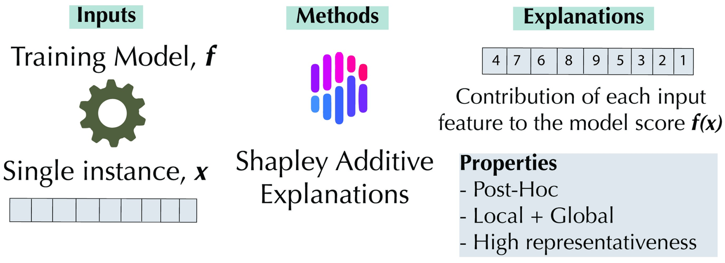
In this study, we combined machine learning (ML) algorithms and SHAP (Shapley Additive Explanations) explanations to analyze dominant features governing properties of one-part geopolymer cements. Figure 2 shows the principle of the method. The input variables include slag content (Slag), Na₂O dosage in the system (Na₂O), activator modulus (Ms), water-to-binder ratio (w/b), sand-to-binder ratio (s/b), curing temperature (Temperature), and curing humidity (Humidity). The target variables are compressive strength at 3, 7, 14, and 28 days (CS_3d, CS_7d, CS_14d, CS_28d) of the one-part geopolymers.

3.1. Machine Learning Methods

We trained six ML models including Random Forest, ExtraTrees, SVR, Ridge, KNN, and XGBoost on the collected dataset. According to the performance of $R^2$, RMSE, and MAE, we selected the best-performing XGBoost as the primary model for subsequent SHAP analysis.

3.1.1. Random Forest (RF)

Random Forest combines bagging with random feature subspaces. Given training data ${\left\{({\mathbf{x}}_i,y_i)\right\}}_{i=1}^n$, draw B bootstrap samples and train a CART regression tree $f_b(·)$ on each. The prediction is the ensemble average:

$$\widehat{y}\left(\mathbf{x}\right)={\displaystyle \frac{1}{B}}\sum _{b=1}^B{f}_b\left(\mathbf{x}\right).$$

(1)

Randomization over data and features decorrelates trees and reduces variance.

3.1.2. Extremely Randomized Trees (Extra Trees)

Extra Trees follows the same tree-ensemble idea as RF but injects additional randomness at each split: for each selected feature, several split thresholds are drawn uniformly at random and the best among these random candidates is chosen. Training uses the full dataset without bootstrap sampling. This typically further lowers variance and speeds up training.

3.1.3. Support Vector Regression (SVR)

SVR applies the maximum-margin principle to regression via an $\epsilon$-insensitive loss. The primal problem is

$$\begin{array}{cc}\hfill \underset{\mathbf{w},b,\xi ,{\xi }^{*}}{min}& {\displaystyle \frac{1}{2}}{\parallel \mathbf{w}\parallel }^2+C\sum _{i=1}^n({\xi }_i+{\xi }_i^{*})\hfill \\ \hfill \mathrm{s}.\mathrm{t}.& y_i-({\mathbf{w}}^{\top }\varphi \left({\mathbf{x}}_i\right)+b)\le \epsilon +{\xi }_i,\hfill \\ \hfill & ({\mathbf{w}}^{\top }\varphi \left({\mathbf{x}}_i\right)+b)-y_i\le \epsilon +{\xi }_i^{*},\hfill \\ \hfill & {\xi }_i,{\xi }_i^{*}\ge 0.\hfill \end{array}$$

(2)

With the kernel trick (e.g., RBF kernel $K(\mathbf{x},{\mathbf{x}}^{\prime })=exp(-\gamma \parallel \mathbf{x}-{\mathbf{x}}^{\prime }{\parallel }^2)$), SVR models smooth nonlinearities.

3.1.4. Ridge Regression

Ridge is linear regression with ${\ell }_2$ regularization to mitigate multicollinearity and overfitting:

$$\underset{\mathbf{w},b}{min}\sum _{i=1}^n{\left(y_i-({\mathbf{w}}^{\top }{\mathbf{x}}_i+b)\right)}^2+\lambda {\parallel \mathbf{w}\parallel }^2.$$

(3)

The solution satisfies $({\mathbf{X}}^{\top }\mathbf{X}+\lambda \mathbf{I})\mathbf{w}={\mathbf{X}}^{\top }\mathbf{y}$. Larger $\lambda$ increases bias and reduces variance. Ridge is stable and computationally efficient but, being linear, cannot capture complex nonlinearities or higher-order interactions without feature engineering.

3.1.5. K-Nearest Neighbors (KNN) Regression

KNN is a non-parametric, instance-based method. To predict at $\mathbf{x}$, find its k nearest neighbors ${\mathcal{N}}_k\left(\mathbf{x}\right)$ (e.g., by Euclidean distance) and average their responses, optionally with distance weights:

$$\widehat{y}\left(\mathbf{x}\right)={\displaystyle \frac{{\sum }_{i\in {\mathcal{N}}_k\left(\mathbf{x}\right)}{w}_i{y}_i}{{\sum }_{i\in {\mathcal{N}}_k\left(\mathbf{x}\right)}{w}_i}},w_i={\displaystyle \frac{1}{{(\mathrm{dist}(\mathbf{x},{\mathbf{x}}_i)+\delta )}^p}}.$$

(4)

KNN requires no explicit training but has prediction costs that grow with the dataset size. It is sensitive to feature scaling and distance choice, and can degrade in high dimensions.

3.1.6. Extreme Gradient Boosting(XGBoost)

XGBoost is a regularized implementation of gradient boosted decision trees. It builds an additive model by iteratively fitting residuals:

$${\widehat{y}}^{\left(t\right)}\left(\mathbf{x}\right)={\widehat{y}}^{(t-1)}\left(\mathbf{x}\right)+\eta f_t\left(\mathbf{x}\right),f_t\in \mathcal{F},$$

(5)

with a second-order, regularized objective:

$${\mathcal{L}}^{\left(t\right)}=\sum _{i=1}^n\left[g_i{f}_t\left({\mathbf{x}}_i\right)+\frac{1}{2}{h}_i{f}_t{\left({\mathbf{x}}_i\right)}^2\right]+\Omega \left(f_t\right),\Omega \left(f\right)=\gamma T+\frac{1}{2}\lambda {\parallel \mathbf{w}\parallel }^2,$$

(6)

where $g_i,h_i$ are the first and second derivatives of the loss at iteration $t-1$, T is the number of leaves, and $\mathbf{w}$ are leaf values. Shrinkage (learning rate), row/column subsampling, and explicit tree regularization control model complexity; sparse-aware splitting and a default direction handle missing values efficiently.

3.2. Shap Analysis

SHapley Additive exPlanations (SHAP) analysis was employed to interpret the influence of input features on the predicted target variables. It is a unified framework for model interpretation based on cooperative game theory, where the contribution of each feature is quantified using the concept of Shapley values. This integration provides a transparent link between material composition, curing conditions, and the resulting mechanical performance. The Shapley value for a feature i (e.g., Na₂O dosage or w/b ratio) is defined as:

$${\varphi }_i=\sum _{S\subseteq N\setminus \left\{i\right\}}{\displaystyle \frac{\left|S\right|!\left(\right|N|-|S|-1)!}{\left|N\right|!}}\left[f(S\cup \{i\left\}\right)-f\left(S\right)\right],$$

(7)

where N is the set of all input features (e.g., Slag, Na₂O, Ms, w/b, s/b, Temperature, Humidity), S is a subset of these features not including i, $f\left(S\right)$ is the model prediction using only features in S, and ${\varphi }_i$ represents the marginal contribution of input feature i across all possible subsets.

The prediction of a target variable, such as compressive strength at 28 days (CS_28d), can then be decomposed as a linear sum of feature contributions:

$$f\left(x\right)={\varphi }_0+\sum _{i=1}^M{\varphi }_i,$$

(8)

where ${\varphi }_0$ is the average model output over the training dataset, and ${\varphi }_i$ denotes the SHAP value for feature i. A positive ${\varphi }_i$ indicates that the feature increases the predicted value relative to the baseline, whereas a negative ${\varphi }_i$ suggests a decreasing effect.

Thus, SHAP provides both global insights into which input variables dominate the prediction of compressive strength, and local interpretations of how individual features affect specific predictions. Importantly, SHAP fairly distributes contributions among correlated variables, thereby mitigating the effects of multicollinearity and enabling a more reliable assessment of feature importance.

4. Results

4.1. Data Distribution Analysis

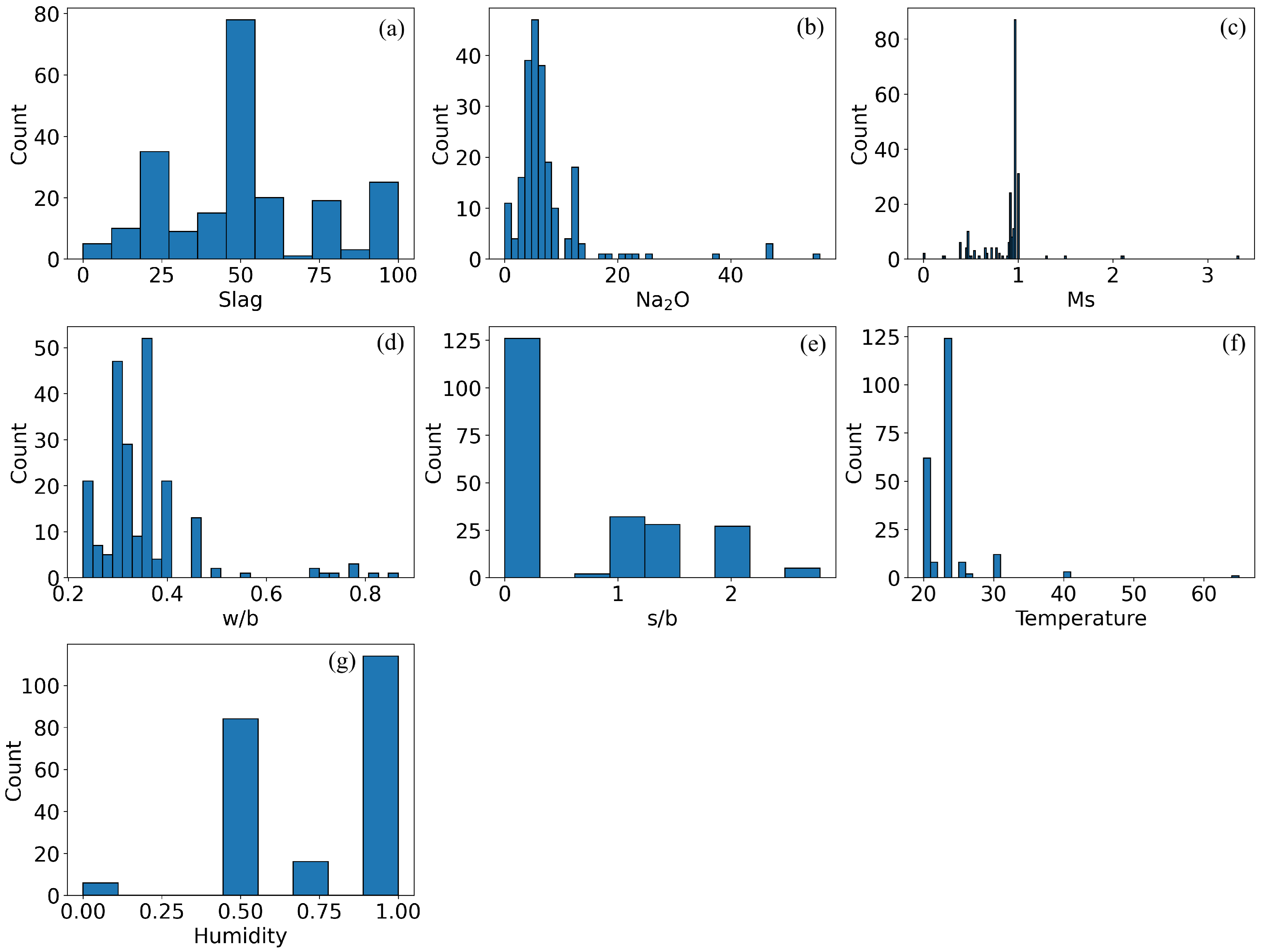
Figure 3 shows the distributions of the seven input variables. Slag content exhibits a relatively uniform spread with peaks around 50%. Na₂O dosage is strongly right-skewed, with most values concentrated below 10%. The modulus Ms is narrowly distributed around 1.0, indicating little variation. The water-to-binder ratio (w/b) is moderately right-skewed, with most values ranging between 0.25 and 0.45. The sand-to-binder ratio (s/b) shows a discrete distribution with several distinct peaks. Curing temperature is heavily concentrated at 20–25 °C, with a few higher values up to 60 °C. Finally, curing humidity displays a bimodal distribution, with most samples clustered between 50% to 100%. Overall, the input variables exhibit diverse distributions, covering a broad range of values, which is beneficial for capturing variable effects in subsequent modeling.

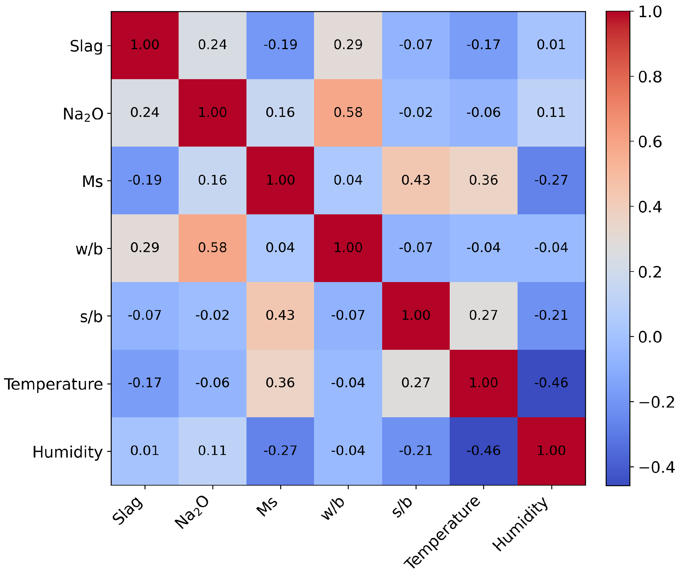
Figure 4 shows the Pearson correlation coefficients among the 7 input variables. The correlation coefficients indicate that most variable pairs show weak or only moderate relationships ($\left|r\right|<0.6$). The strongest positive correlation is observed between Na₂O dosage and the water-to-binder ratio ($r=0.58$), followed by moderate correlations between Ms and s/b ($r=0.43$) and between Ms and Temperature ($r=0.36$). On the other hand, the most pronounced negative correlation is found between Humidity and Temperature ($r=-0.46$). Overall, the correlations are relatively low, suggesting that no severe multicollinearity exists among the input variables. This finding is important because high collinearity can obscure the contribution of individual variables in machine learning models and reduce their generalization performance. Since the observed correlation levels remain within acceptable ranges, all seven variables (slag content, Na₂O dosage, activator modulus Ms, water-to-binder ratio, sand-to-binder ratio, curing temperature, and curing humidity) can be retained as independent input features for subsequent modeling without the need for dimensionality reduction or variable elimination.

As for the target variables, it should be noted that not all target variables were measured in the 220 records. As illustrated in Figure 5a, in most cases, only a subset of the targets was available: 107 experiments reported compressive strength at 3 days, 188 experiments included compressive strength at 7 days, 38 experiments provided compressive strength at 14 days, and 215 experiments recorded compressive strength at 28 days. Figure 5b illustrates the distributions of four target variables, including compressive strength at different curing ages (3-day, 7-day, 14-day, 28-day). The red dot denotes the median. Compressive strength increases with curing age, with mean values of 30.83 MPa (CS_3d), 37.35 MPa (CS_7d), 33.04 MPa (CS_14d), and 48.90 MPa (CS_28d). CS_28d exhibits the largest variation. Noted that $C{S}_{14}$ appears lower than others. This anomaly is attributed to the small number of available 14-day strength data points in the dataset rather than an actual reduction in compressive strength at 14 days.

4.2. Machine Learning–Based Estimation of Material Properties

Six ML regressors were used to train the collected dataset firstly: Random Forest, ExtraTrees, SVR, Ridge, KNN, and XGBoost. The hyperparameters of all six machine learning models were optimized using a grid search strategy, which systematically explored predefined parameter ranges and selected the best-performing combination based on cross-validation results. Model performance was evaluated through k-fold cross-validation ($k=5$), where the dataset was randomly split into five folds, and the average performance across all folds was reported. All training and validation were conducted in a computing environment equipped with an Intel Core i7 processor, 16 GB RAM, Windows 11, and Python 3.13, using the Scikit-learn, XGBoost, and SHAP libraries.

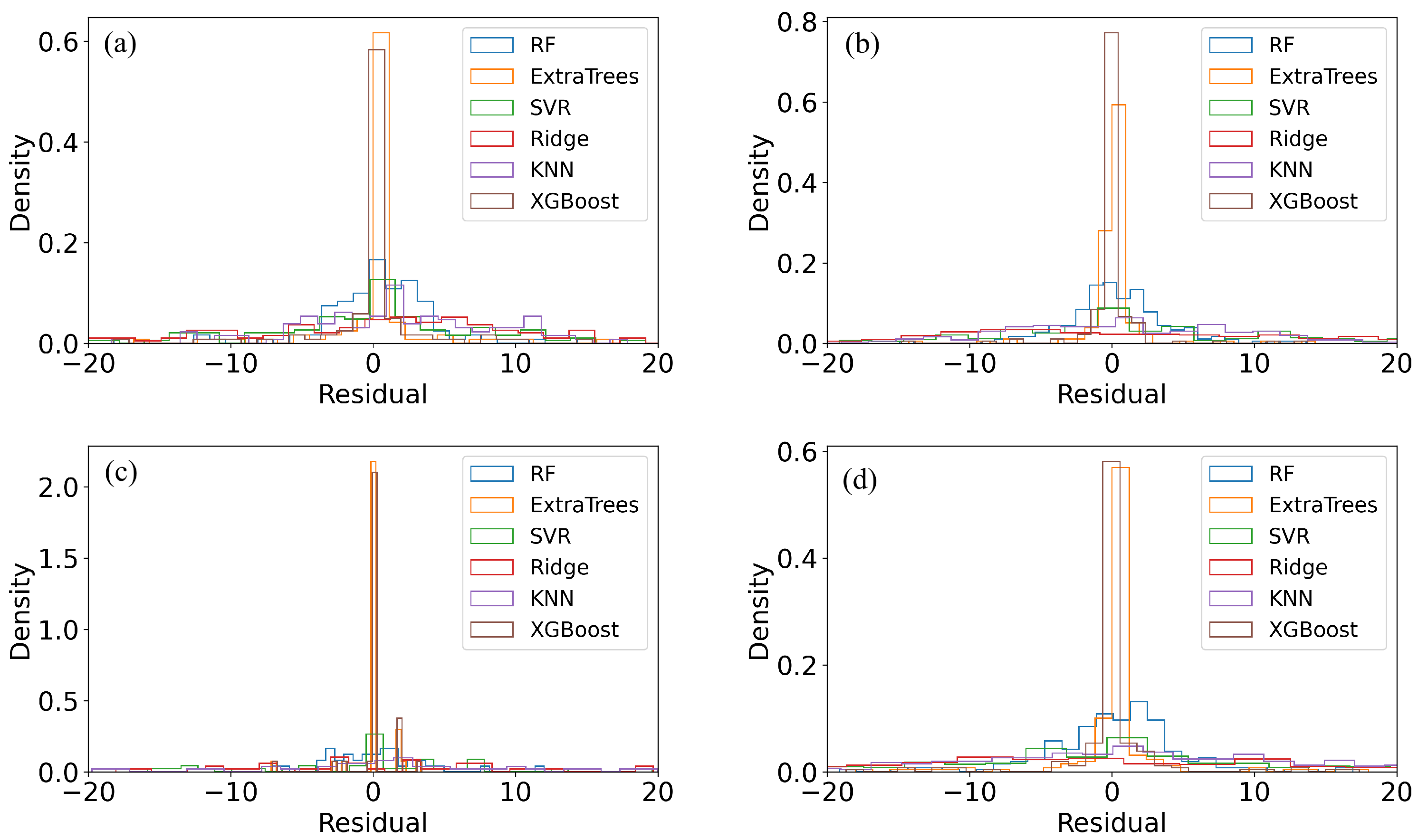
Figure 6 presents the residual distributions of all six models for the four target variables. Across all six targets, ExtraTrees and XGBoost produce residuals that are visibly more concentrated around zero—narrower spread and fewer large deviations—than the other methods. Random Forest typically follows as a close second tier. SVR and KNN deliver intermediate behavior that depends on the target’s smoothness and local structure. Ridge consistently exhibits the widest residual spread, indicating underfitting due to its linear functional form. These observations are aligned with the intuition that tree ensembles better capture nonlinearities and higher-order interactions among the seven input features.

Figure 7 summarizes the $R^2$, RMSE and MAE performance of the 6 predictive models in a radar chart, whose formulas are as follows:

$$R^2=1-{\displaystyle \frac{{\sum }_{i=1}^n{(y_i-{\widehat{y}}_i)}^2}{{\sum }_{i=1}^n{(y_i-\overline{y})}^2}},$$

(9)

$$RMSE=\sqrt{{\displaystyle \frac{1}{n}}{\sum }_{i=1}^n{(y_i-{\widehat{y}}_i)}^2},$$

(10)

$$MAE={\displaystyle \frac{1}{n}}\sum _{i=1}^n\left|y_i-{\widehat{y}}_i\right|,$$

(11)

where $y_i$ and ${\widehat{y}}_i$ denote the observed and predicted values, respectively, $\overline{y}$ is the mean of the observed values, and n is the number of data points. These statistics were obtained from a k-fold cross-validation procedure, where the dataset was randomly partitioned into k subsets; in each iteration, one subset was used as the validation set and the remaining $k-1$ subsets were used for training. The reported values represent the average performance across all validation folds. XGBoost and ExtraTrees show almost overlapping $R^2$ profiles and clearly outperform the other models, followed by Random Forest with consistently lower yet competitive scores. Ridge is the weakest overall (often failing to reach a practically useful $R^2$), while SVR and KNN sit in between depending on the target. Tree ensembles (RF, Extra Trees, XGBoost) are robust to feature scaling and capture nonlinearities and interactions; RF/Extra Trees primarily reduce variance through randomness, while XGBoost balances bias and variance via additive boosting and strong regularization. SVR is competitive on small- to medium-sized datasets with smooth targets but requires careful scaling and tuning. Ridge provides a fast, stable linear baseline with limited expressive power. KNN is simple and local but sensitive to distance metrics and dimensionality. Given the above, we select XGBoost as the primary model for subsequent interpretation with SHAP. Tree-based SHAP (TreeExplainer) is computationally efficient and faithful for gradient-boosted trees, enabling us to quantify global effects while retaining strong predictive performance.

Table 2. The evaluation metrics $R^2$, RMSE, and MAE of all prediction models.

	Model	CS_3d	CS_7d	CS_14d	CS_28d
$R^2$	ExtraTrees	0.9464	0.9888	0.9918	0.9804
	KNN	0.8141	0.8100	0.7304	0.8061
	RF	0.9325	0.9671	0.9572	0.9648
	Ridge	0.5794	0.4671	0.7304	0.4312
	SVR	0.7022	0.7151	0.8132	0.6978
	XGBoost	0.9462	0.9889	0.9918	0.9810
RMSE	ExtraTrees	3.7715	2.1520	1.5378	3.5557
	KNN	7.0253	8.8473	8.8329	11.1718
	RF	4.2327	3.6825	3.5211	4.7606
	Ridge	10.5668	14.8159	8.8329	19.1363
	SVR	8.8910	10.8330	7.3523	13.9485
	XGBoost	3.7796	2.1695	1.5384	3.5723
MAE	ExtraTrees	1.6148	0.6360	0.6328	1.2395
	KNN	5.5770	6.9305	6.6341	8.7905
	RF	2.8452	2.6556	2.6092	3.3540
	Ridge	8.2062	11.7629	7.1553	15.0461
	SVR	6.0249	7.7845	5.1732	10.0671
	XGBoost	1.6692	0.7875	0.6517	1.4226

illustrates the detail evaluation metrics $R^2$, RMSE, and MAE of all prediction models including KNN, RF, Ridge, SVR, and XGBoost for the compressive strengths at 3-day, 7-day, 14-day, and 28-day. As have been discussed in the result section, XGBoost and ExtraTrees have the best performance. Ridge exhibits the worst performance.

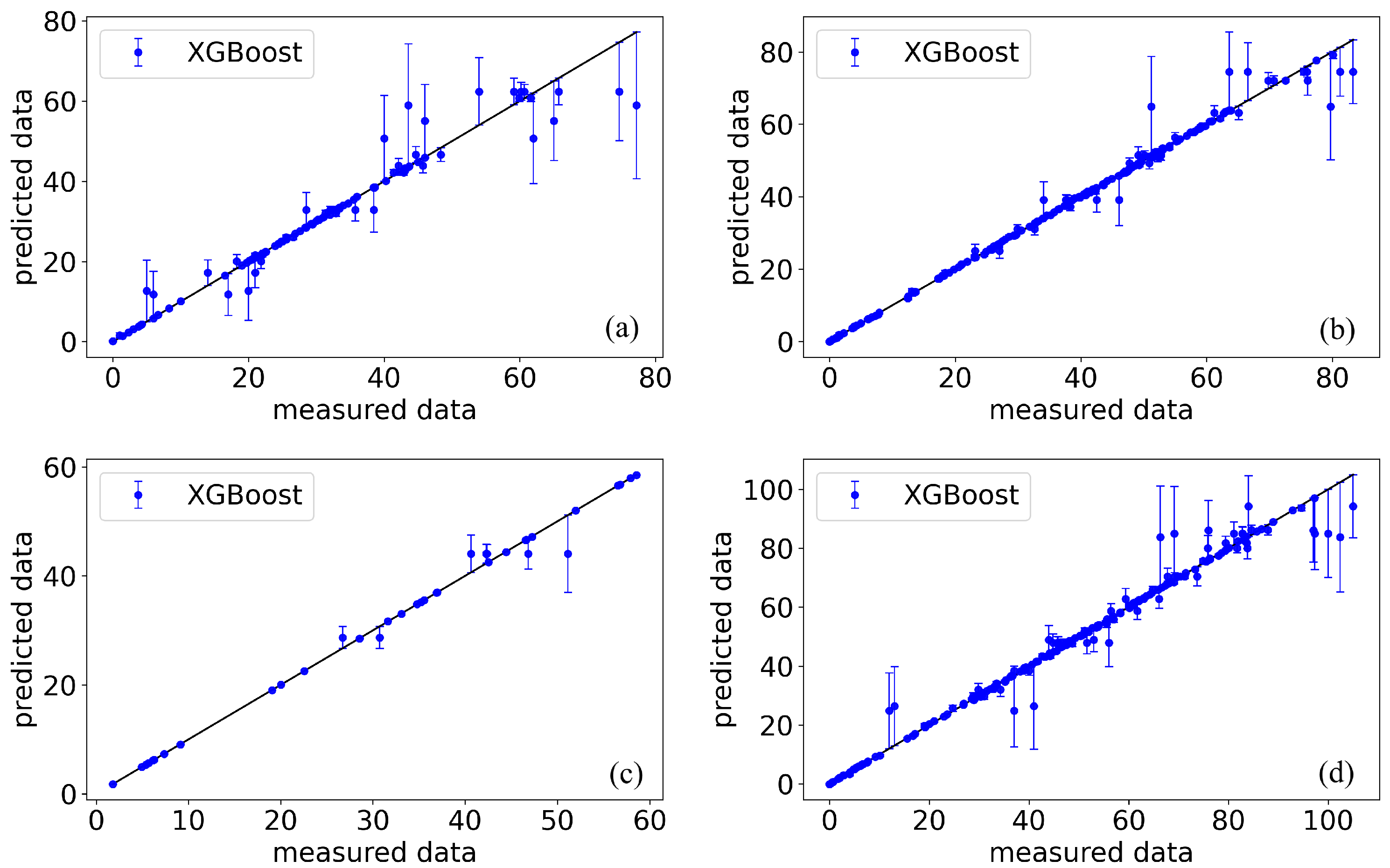
As XGBoost achieved the top performance across targets (see Figure 6 and Figure 7 and Table 2), we use XGBoost as the primary interpretation model. Figure 8 illustrates the predicted versus measured data from the best-performing XGBoost model. In the measured–predicted plots, points are shown for the best-performing XGBoost model with vertical error bars representing absolute residuals. Visual alignment of points along the $y=x$ line and uniformly short error bars across the range suggest low bias and variance for XGBoost on all four targets. Occasional departures from the diagonal indicate localized regimes where the function is more complex or sparsely sampled, motivating subsequent feature-attribution analysis.

4.3. SHAP-Based Feature Importance Interpretation

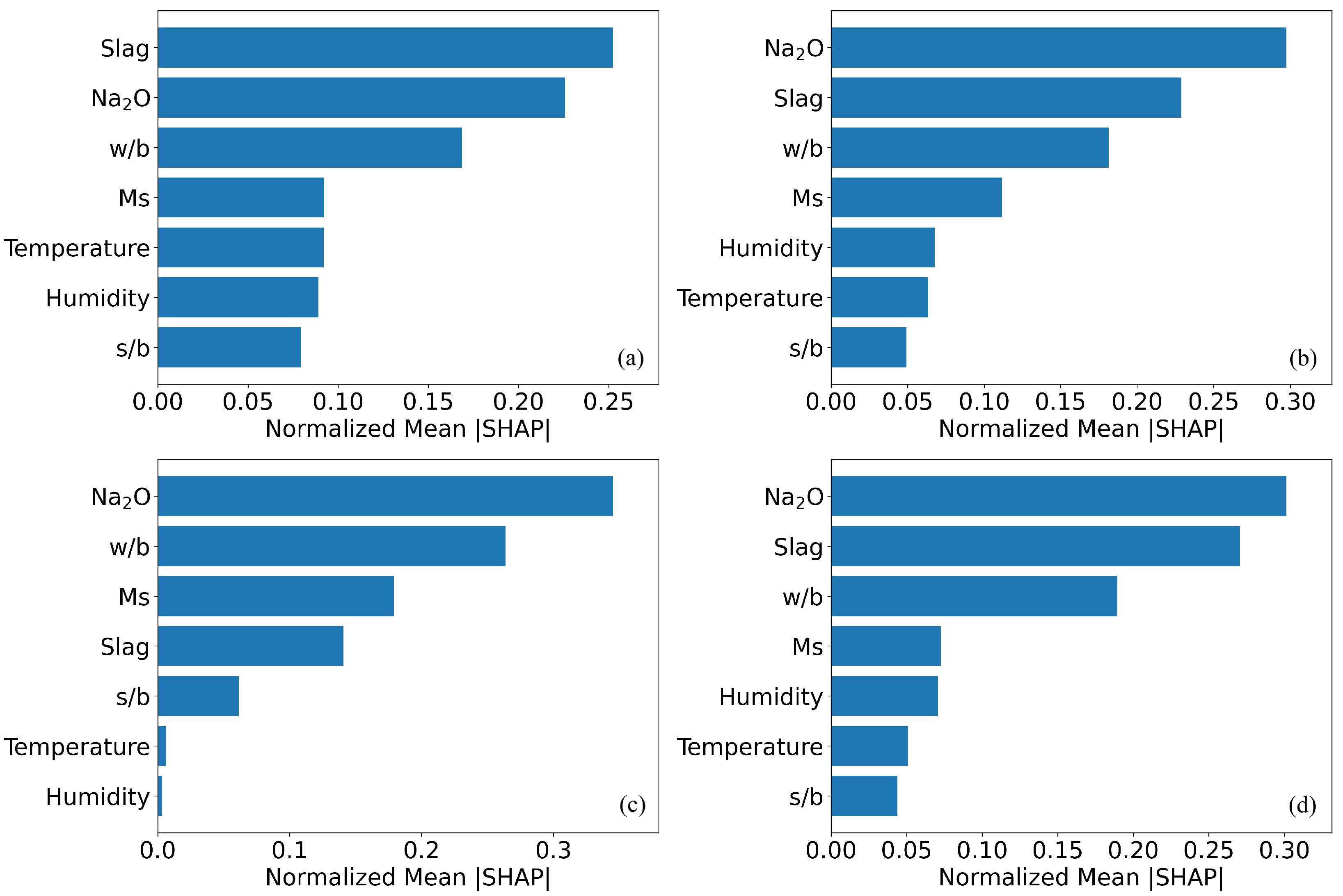
Figure 9 illustrates the normalized feature importance for the four target variables. For the 3-day compressive strength CS_3d, the normalized importance of Slag = 0.25 (highest), Na₂O = 0.23, w/b = 0.17, Ms = 0.09, s/b = 0.08, Temperature = 0.09, Humidity = 0.09. Thus, Slag governs the 3 d response—consistent with Ca-rich slag supplying ${Ca}^{2+}$ to rapidly form C–(N)–A–S–H; sufficient Na₂O ensures high pH and soluble silicate to drive dissolution/gelation, while w/b controls porosity and ion transport. For the 7-day compressive strength CS_7d, Na₂O = 0.30 > Slag = 0.23 > w/b = 0.18 By mid-early age, the alkalinity/soluble-silicate supply becomes the dominant rate controller for dissolution and gel growth. For the 14-day compressive strength CS_14d, Na₂O = 0.35 > w/b = 0.26 > Ms = 0.18 (Slag = 0.14, s/b = 0.06, Temperature = 0.01, Humidity = 0.00). The reaction remains alkalinity-driven, with the alkali-activated reaction of the aluminosilicate precursor entering a steady stage, while the w/b exerts an indirect and sustained influence on late-age strength by determining the initial structural compactness. For the 28-day compressive strength CS_28d, Na₂O = 0.30 and Slag = 0.27 are the top two; w/b = 0.19 (Ms = 0.07, s/b = 0.04, Temperature = 0.05, Humidity = 0.07). Late-age strength is capped by slag-derived Ca enabling denser C–(N)–A–S–H networks, while adequate Na₂O ensures earlier-age reaction completion to unlock that potential.

In one-part geopolymers (OPGs), adding water dissolves the solid activator and releases ${OH}^{-}$/${Na}^{+}$ and soluble silicate, which drive precursor dissolution and the formation of a C–(N)–A–S–H–dominated gel network. The relationship between water-to-binder ratio (w/b) and compressive strength in this study shows a generally decreasing trend over the range of values considered. Although an optimum w/b ratio may exist in broader formulations, it was not evident in the present dataset, which mainly covers the relatively low w/b region typical of one-part geopolymer mixtures. The activator modulus Ms (SiO₂/Na₂O) tunes the silicate/alkalinity balance and typically has an optimum window. Within the ranges studied here, s/b and curing temperature/humidity play secondary roles. It should be noted that the relatively low importance of temperature and relative humidity primarily reflects the narrow ranges of these variables in the dataset (temperature: 20–25 °C; humidity: 50% and 100%), rather than a definitive mechanistic conclusion. Therefore, their influence should be interpreted with caution. Microstructural characterization data in the literature also support this trend. XRD and SEM analyses indicate that Na₂O, by accelerating precursor dissolution and polycondensation, promotes the formation of (N,C)-A-S-H gels at intermediate ages, thereby contributing to strength [18,34]. Calorimetry results show that early-age geopolymerization rates are largely governed by ${Ca}^{2+}$ content (slag being the primary source of ${Ca}^{2+}$); an increase in ${Ca}^{2+}$ concentration induces the formation of more Si–Al oligomers, which in turn enhances early strength [35]. FTIR and SEM results confirm that increased slag content significantly promotes the geopolymerization of fly ash at later ages, increases gel yield, and improves matrix densification [12,15,16].

As shown in Figure 10, across all outputs, the first four inputs—Slag, Na₂O, Ms, and w/b—consistently dominate, while s/b, Temperature, and Humidity remain secondary. The combined shares of the first four are CS_3d = 0.74, CS_7d = 0.82, CS_14d = 0.93, and CS_28d = 0.83. In contrast, the last three sum to 0.26, 0.18, 0.07, 0.16, and 0.17, respectively. Mechanistically, this reflects that mix/chemistry controllers (Na₂O and Ms for alkalinity/soluble silicate; Slag for Ca supply/gel yield; w/b for pore structure and transport) govern the reaction and microstructure, whereas s/b and ambient factors only weakly perturb performance within the tested ranges. This may also be attributed to two factors: first, siliceous sand is an inert material that does not participate in chemical reactions; second, the curing temperature and humidity data exhibit a relatively concentrated distribution (temperature: 20–30 °C; humidity: 50%, 75% and 100%), which limits their observable impact within the tested ranges. In addition, the weak sensitivity of s/b may partly reflect the limited experimental variation of this parameter: as shown in Figure 3e, its values are concentrated around a few discrete peaks, which constrains the model’s ability to capture potential indirect effects such as changes in packing density or water distribution. The leading factors evolve with age: at CS_3d, slag = 0.25 is the largest share (Na₂O = 0.23, w/b = 0.17, Ms = 0.09), consistent with Ca-rich slag rapidly forming C–(N)–A–S–H; by CS_7d and CS_14d, Na₂O leads (0.30 and 0.35) as alkalinity/soluble-silicate supply controls dissolution–gelation, with w/b strengthening its role at 14-day (0.26) and Ms = 0.18 indicating a modulus window. At CS_28d, Slag = 0.27 and Na₂O = 0.30 jointly cap the attainable strength, with w/b = 0.19 continuing to shape porosity.

From Figure 11, it can be seen that the four strength targets show the same directional pattern: samples with high Na₂O and high Slag mostly lie to the right (positive SHAP leads to raising strength), whereas w/b samples are also concentrated on the right but correspond to low w/b ratios (contributing positively to strength). The age dependence is also clear. At 3-day, Slag dominates the positive side, consistent with Ca-rich slag rapidly supplying ${Ca}^{2+}$ to form and densify the C-(N)-A-S-H network; by 7–14 day, Na₂O becomes the lead driver as alkalinity/soluble-silicate supply controls dissolution–gelation, and the role of w/b grows (more porosity control at 14-day). At 28-day, Slag strengthens again alongside Na₂O, indicating the late-age ceiling is set by Ca-enabled densification while early alkali availability ensures sufficient reaction completion. Across ages, Ms spreads to both sides (too low or too high modulus weakens contributions), whereas Temperature, Humidity, s/b cluster near zero in this dataset.

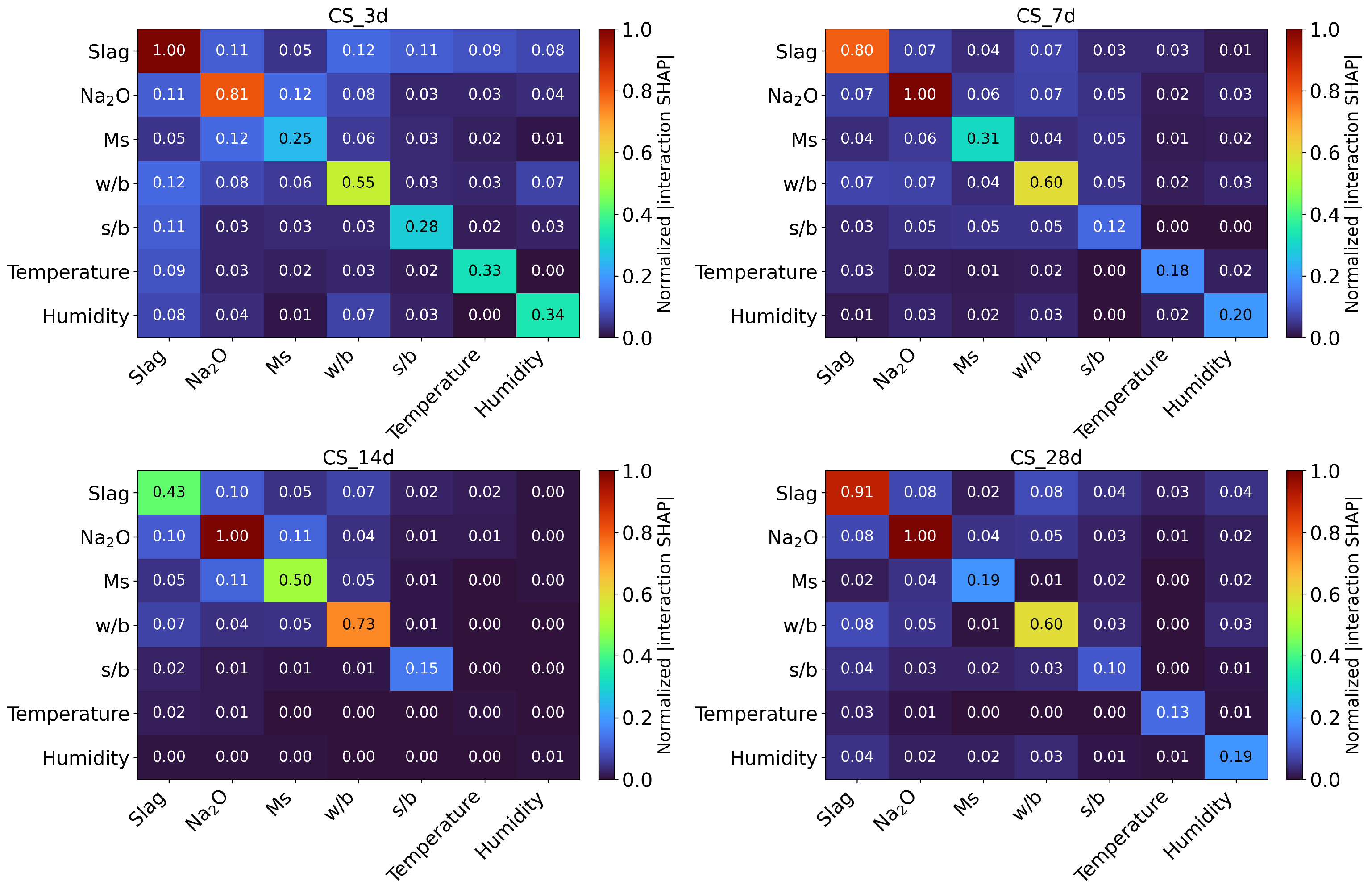
Figure 12 shows the impact of interaction among each variable on each target. Each panel is a symmetric matrix showing the normalized mean $\left|\mathrm{interaction}\mathrm{SHAP}\right|$ for one target. Diagonal cells represent each feature’s main-effect magnitude, while off-diagonals quantify pairwise interaction strength. Across all targets, the strongest off-diagonal interaction is Slag × Na₂O, reflecting synergy between Ca supply (slag) and alkalinity/soluble silicate (Na₂O): raising Slag pays off most at moderate Na₂O, whereas too little or too much alkalinity limits densification. A consistent secondary interaction is $M_s\times$ Na₂O, highlighting the combined role of silicate speciation (tuned by $M_s$) and alkalinity (set by Na₂O). Environmental couplings are generally small, but at early age (CS_3d) they are more visible, consistent with thermal/moisture effects amplifying dissolution and drying; by CS_28d they shrink (typical Temperature-related entries 0.13 to 0.20). Optimization should first co-tune Slag and Na₂O (the strongest interaction window), then coordinate $M_s\times$ Na₂O.

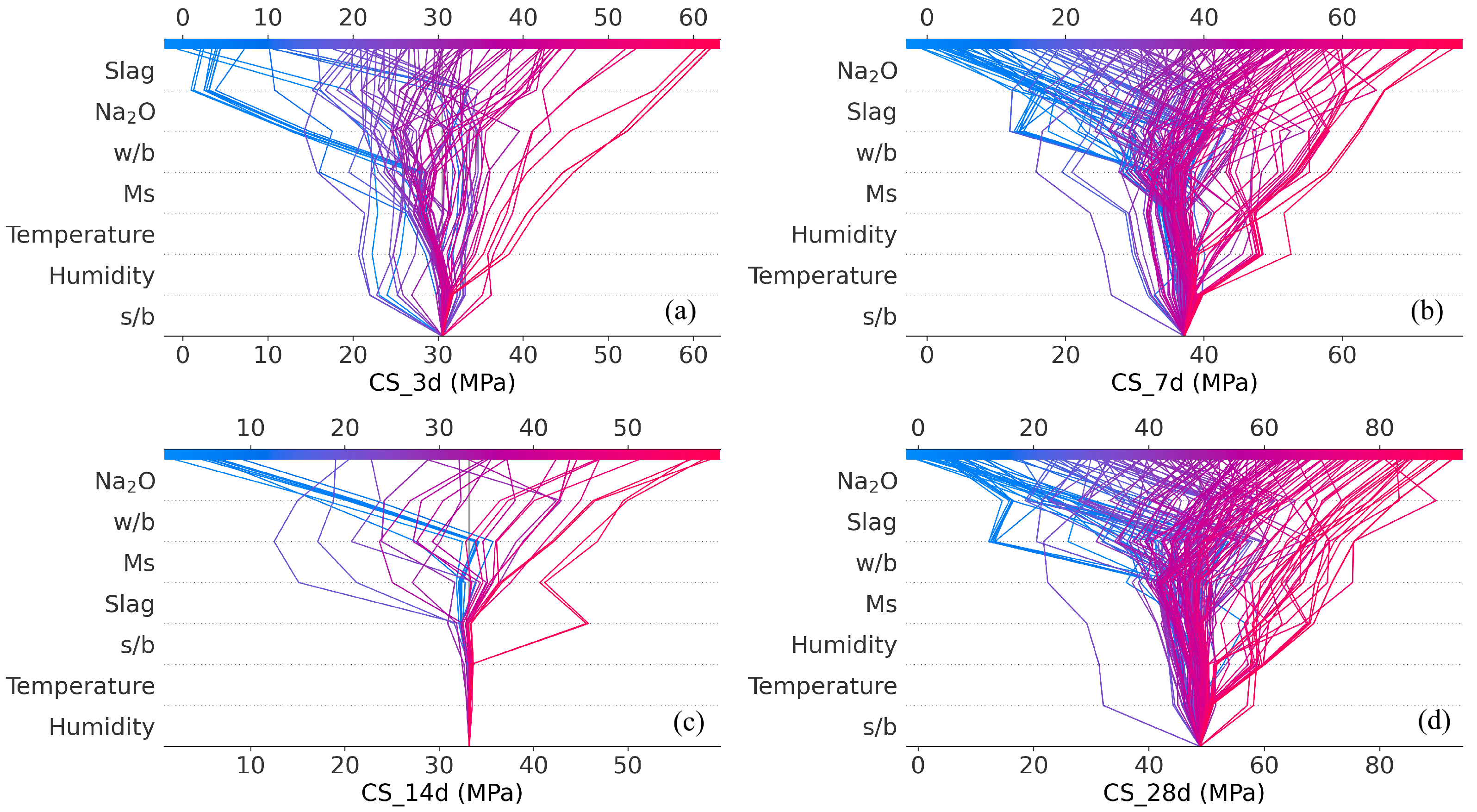
In Figure 13, for every sample, the cumulative SHAP path from the baseline prediction to the final model output as features are added from top to bottom. The horizontal axis shows the attainable range for each target. Wide horizontal shifts at a given feature indicate large marginal effects; narrow, near-vertical segments indicate weak effects. The fan-shaped spread of paths after key features captures sample-to-sample heterogeneity and interactions among variables (e.g., different combinations of Na₂O, Slag, and w/b produce different cumulative trajectories), which is consistent with the pairwise interaction heatmaps in Figure 12.

The typical high-strength trajectory is: Na₂O gives the first positive lift, Slag adds another positive lift, and w/b introduces a partial pull-back (negative contribution). This ordering matches the mechanism that alkalinity controls reaction rate, Ca supply from slag controls gel densification, and w/b governs pore structure and transport. We can see this shift in dominance across ages: at 3-day, the largest lateral spread is concentrated at Slag (Ca-driven early gel formation), at 7 and 14 day the largest shift moves to Na₂O (rate control via pH/soluble silicate), and by 28 d the large positive shifts appear again at both Slag and Na₂O (densification plus sufficient earlier-age reaction). Overall, the decision routes turn the bar/heatmap rankings into step-by-step, sample-resolved stories: they show where along the feature sequence the prediction is won or lost and how strongly chemistry (Na₂O, Slag) and pore-structure control (w/b) shape each target.

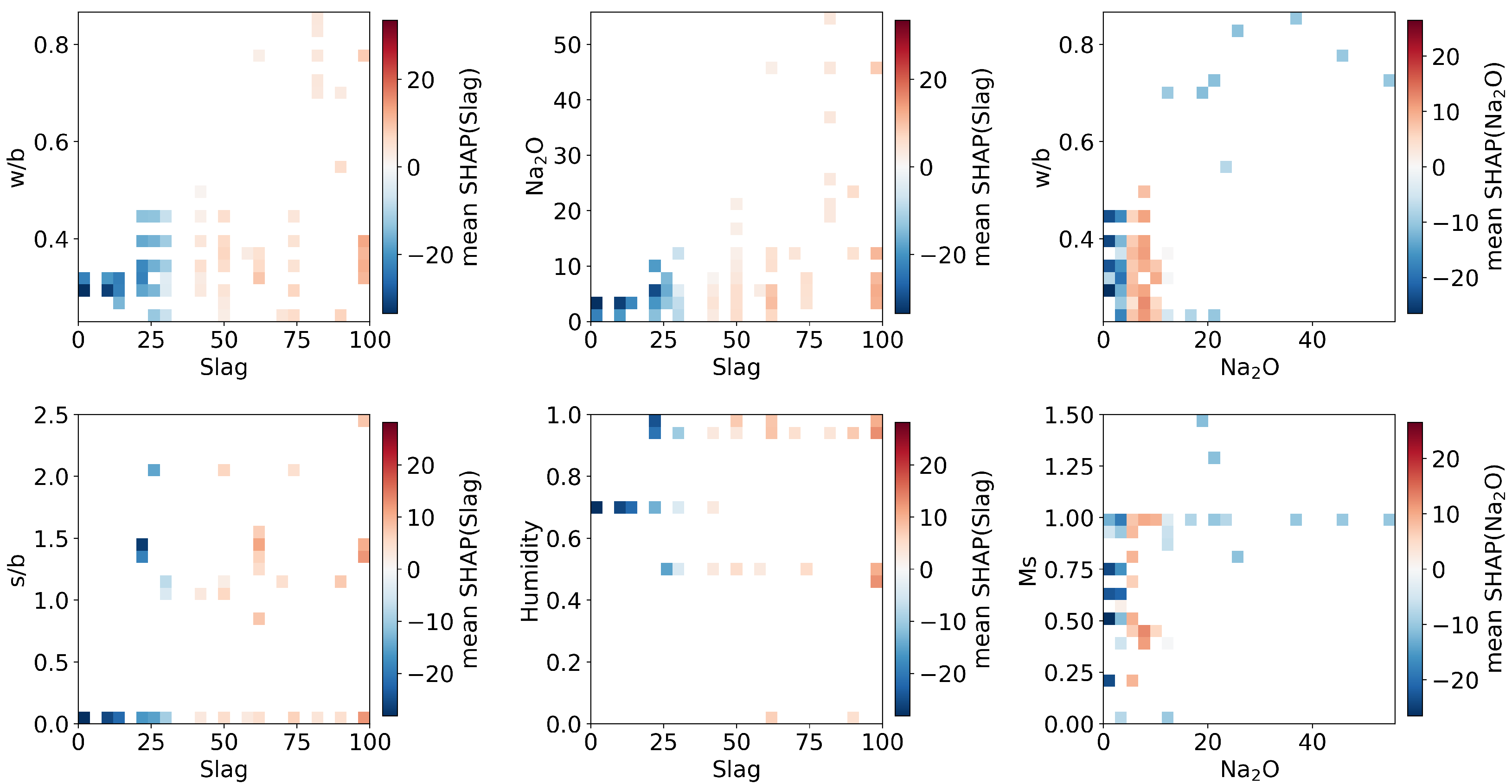
Figure 14 shows the two-dimensional (2D) dependence of the top-six interacting feature pairs for the 28-day compressive strength. Axes display the raw feature values; the colormap encodes the mean SHAP of the x-axis feature, with red indicating a positive contribution to the predicted strength, blue indicating a negative contribution, and pale cells corresponding to bins with few samples. The maps reveal a consistent chemistry–porosity coupling: for Slag × w/b, Slag contributes positively at low w/b and medium–high Slag contents, but its benefit collapses and can turn negative at high w/b. For Slag × Na₂O, increasing Slag is most effective at moderate Na₂O; very low Na₂O (or very low Slag) drives the contribution negative. While Slag and Na₂O consistently emerged as the dominant factors across ages, it should be noted that the positive effect of Na₂O diminishes at higher w/b. Therefore, the recommendation to prioritize Slag and Na₂O while controlling w/b reflects an overall trend within the studied ranges rather than a universal rule under all conditions. For Na₂O × w/b, Na₂O is beneficial under low w/b and moderate Na₂O, whereas high w/b suppresses or reverses the effect. For Slag × s/b, positive contributions cluster at low s/b, implying filler dilution weakens slag’s benefit as s/b rises. Slag × Humidity shows a milder coupling in which wetter conditions combined with higher Slag more often yield positive contributions. Finally, Na₂O × Ms exhibits a modulus window: Na₂O helps most around intermediate Ms, while very low/high Ms or very low Na₂O weaken or invert the contribution. These patterns are consistent with the mechanism that alkalinity (Na₂O) governs reaction rate, Ca supply (Slag) controls late-age densification, and w/b shapes pore structure. Note that only the 28-day strength is discussed in the main text. The corresponding 2D-dependence plots for the other targets (CS_3d, CS_7d, CS_14d) are provided in the Appendix A (See Figure A1, Figure A2 and Figure A3). In addition, sparsely populated regions in the 2D SHAP dependence maps (pale cells, e.g., high Ms combined with low w/b) rely more on extrapolation than dense data support. Therefore, the SHAP values in these zones should be interpreted with caution, and additional experiments will be needed to validate these trends.

5. Discussions

5.1. Strengths of the Present Study

Previous applications of machine learning in geopolymer research have primarily focused on predicting 28-day compressive strength, often using artificial neural networks (ANN), support vector machines, or tree-based methods. While these studies demonstrated the feasibility of ML for strength prediction, they generally lacked interpretation of early-age strength development and provided limited mechanistic insights. In contrast, the present study systematically analyzes compressive strength at four ages (3, 7, 14, and 28 days), thereby offering a more complete picture of strength evolution in one-part geopolymers. Moreover, by evaluating six candidate algorithms and selecting XGBoost as the best-performing model ($R^2>0.9$ for most targets), we demonstrate superior predictive accuracy compared to other 5 methods. Importantly, the integration of SHAP goes beyond global feature ranking by quantifying feature interactions (e.g., Slag × Na₂O, $M_s\times$ Na₂O), which has not been systematically reported in prior geopolymer ML studies. This methodological advance provides a stronger link between statistical predictions and mechanistic interpretation.

The present study offers several notable strengths. First, it addresses the research gap of multi-age prediction by simultaneously analyzing 3-day, 7-day, 14-day, and 28-day compressive strengths, whereas most prior studies restricted interpretation to a single age (typically 28 days). Second, by assembling a dataset of 220 records from 26 published studies, we provide one of the most comprehensive data-driven analyses of one-part geopolymers to date. Third, the combined XGBoost+SHAP framework enables not only accurate prediction but also transparent interpretation of the roles and interactions of key parameters, which can inform both scientific understanding and practical mix design. Finally, this framework is general and can be extended to other precursor systems and binder technologies, suggesting broad applicability beyond the present dataset.

5.2. Limitations

First, the dataset for 14 day compressive strength is relatively small, so both model accuracy and SHAP attributions for this target are less certain than for the other outputs. More generally, the fidelity of all SHAP results scales with data volume and coverage; sparsely populated regions in the 2D dependence maps (light cells) indicate limited support and should not be over-interpreted. Second, SHAP explains the model, not the world: attributions are conditional on the fitted XGBoost and the observed covariate distribution. Strong correlations or structural constraints among inputs can blur unique causal roles. Third, it should also be noted that some input variables exhibit moderate correlations, such as Na₂O and w/b (r = 0.58). In such cases, SHAP attributions may be influenced by shared variance, with contributions distributed across correlated features. As a result, the importance values should be interpreted as reflecting overall trends rather than strict causal separations between variables. Future work with more balanced datasets and carefully designed experiments will be necessary to disentangle correlated effects and provide more definitive mechanistic validation. Finally, our interaction heatmaps are panel-wise min–max normalized (0–1), which is appropriate for within-target comparison but not for cross-target magnitude comparisons.

5.3. Future Works

To increase robustness and practical utility, we see three immediate avenues. First, we will expand the dataset, especially CS_14d, with a more balanced factorial coverage of Slag, Na₂O, $M_s$, and w/b. Active-learning or optimal-design strategies can be used to target under-sampled regions highlighted by the 2D SHAP maps. In particular, combinations such as high Slag with moderate Na₂O and intermediate $M_s$ under low w/b currently lack sufficient data support, and should be prioritized in future experiments. It will also be necessary to include replicates to quantify measurement noise, and to broaden temperature/humidity ranges to better probe environmental sensitivities. Second, we aim to experimentally validate SHAP-identified interaction windows (e.g., intermediate $M_s$ under low w/b; moderate Na₂O with higher Slag) through targeted mix designs and comprehensive microstructural characterization (XRD, FTIR, NMR, MIP, SEM). This will allow us to confirm the causal pathways inferred from the model. Third, we plan to build a multi-objective optimizer that incorporates multiple performance criteria (strength at different ages, $t_{\mathrm{ini}}$, $t_{\mathrm{fin}}$, cost, and embodied CO₂), combined with constraints on workability and durability. By coupling the trained ML model with counterfactual and Individual/ALE profiles, we aim to propose actionable mix adjustments with quantified uncertainty bounds. Moreover, extending the dataset to alternative precursors (e.g., metakaolin, rice husk ash) will be necessary to avoid misleading extrapolations and to broaden the applicability of the present modeling framework.

In short, the present analysis provides a coherent, mechanism-consistent map of where strengths are gained or lost in OPGs, while also making clear that data sufficiency—most notably for CS_14d—and out-of-domain generalization are the primary limits. Addressing these through deliberate data acquisition, uncertainty-aware modeling, and mechanistic validation should yield more reliable prescriptions for mix design and process control.

6. Conclusions

This study applied six machine learning algorithms (Random Forest, ExtraTrees, SVR, Ridge, KNN, and XGBoost) to model the compressive strength of one-part geopolymers (OPGs), and adopted XGBoost as the primary model for SHAP-based interpretability analysis. Within the scope of the collected dataset and tested parameter ranges, the following conclusions can be drawn:

First, four mix parameters—Slag, Na₂O, activator modulus ($M_s$), and water-to-binder ratio (w/b)—consistently showed the highest importance across all target strengths. In contrast, sand-to-binder ratio (s/b), curing temperature, and curing humidity played secondary roles within the studied ranges. Second, strength development follows an age-dependent pattern. At 3 days, Slag had the largest influence; at 7–14 days, Na₂O dominated; and by 28 days, both Slag and Na₂O jointly controlled strength. The variable w/b contributed consistently at all ages by regulating porosity. Third, SHAP interaction analysis revealed that $M_s\times$ Na₂O and Slag × Na₂O were the most significant interaction pairs, reflecting the combined roles of silicate content and alkalinity, and the synergy between Ca supply and alkalinity, respectively. These interpretations are consistent with mechanisms reported in prior literature, but no new experimental phase identification was performed in this work. For strength-oriented mix design, Slag and Na₂O should be prioritized, with w/b kept sufficiently low to maintain compactness. Joint tuning of $M_s$ with Na₂O offers a means to balance reactivity and reaction rate. Since s/b, temperature, and humidity appeared secondary in the present dataset, the main performance levers under similar curing regimes are Slag, Na₂O, $M_s$, and w/b.

To further enhance robustness and generalization, future studies should (i) expand the dataset to underrepresented ages (particularly 14 days) and broader curing conditions, (ii) incorporate alternative aluminosilicate precursors such as metakaolin or rice husk ash, and (iii) perform targeted experimental validation (XRD, FTIR, SEM-EDS, NMR) to directly link SHAP-derived attributions with phase assemblages and microstructural evolution. Combining XGBoost+SHAP with such mechanistic validation and uncertainty quantification will provide more reliable decision support for OPG mix design and performance optimization.

References

1. Yang, Y.; Zhang, J.; Fu, Y.; Long, W.; Dong, B. Synthesis of one-part geopolymers from alkaline-activated molybdenum tailings: Mechanical properties and microstructural evolution. J. Clean. Prod. 2024, 443, 141129. [Google Scholar] [CrossRef]
2. Luukkonen, T.; Abdollahnejad, Z.; Yliniemi, J.; Kinnunen, P.; Illikainen, M. One-part alkali-activated materials: A review. Cem. Concr. Res. 2018, 103, 21–34. [Google Scholar] [CrossRef]
3. Chen, C.; Shenoy, S.; Li, L.; Tian, Q.; Zhang, H. Preparation of one-part geopolymers using coal gasification slag: Effect of alkali fusion product additive and liquid/solid ratio. J. Ind. Eng. Chem. 2024, 137, 207–215. [Google Scholar] [CrossRef]
4. Abiodun, Y.O.; Olanrewaju, O.A.; Gbenebor, O.P.; Ochulor, E.F.; Obasa, D.V.; Adeosun, S.O. Cutting cement industry CO2 emissions through metakaolin use in construction. Atmosphere 2022, 13, 1494. [Google Scholar] [CrossRef]
5. Ali, M.; Saidur, R.; Hossain, M. A review on emission analysis in cement industries. Renew. Sustain. Energy Rev. 2011, 15, 2252–2261. [Google Scholar] [CrossRef]
6. Carneiro, G.; Bier, T.; Waida, S.; Dous, A.; Heinemann, S.; Herr, P.; Charitos, A. Treatment of Energy from Waste Plant fly-ash for blast furnace slag substitution as a Supplementary Cementitious Material. J. Clean. Prod. 2025, 490, 144693. [Google Scholar] [CrossRef]
7. Li, B.; Li, K.H.; Zhou, Y.W.; Xu, H.; Zhao, C.H.; Yu, Y.; Li, Z.C. Nano-mechanism of graphene oxide reinforced fly ash-slag based geopolymer materials to form high polymerization degree C-(A)-SH: A new view of physical-chemical synergistic effect. Cem. Concr. Compos. 2025, 157, 105937. [Google Scholar] [CrossRef]
8. Çelik, A.İ.; Karalar, M.; Aksoylu, C.; Mydin, M.A.O.; Althaqafi, E.; Yılmaz, F.; Umiye, O.A.; Özkılıç, Y.O. Effect of GBFS ratio and recycled steel tire wire on the mechanical and microstructural properties of geopolymer concrete under ambient and oven curing conditions. Case Stud. Constr. Mater. 2024, 21, e03890. [Google Scholar] [CrossRef]
9. Celik, A.I.; Tunc, U.; Karalar, M.; Şahan, M.F.; Özkılıç, Y.O. Study on mechanical, dynamic impact, and microstructural properties of eco-friendly geopolymer paving stones cured in ambient conditions. Constr. Build. Mater. 2025, 464, 140132. [Google Scholar] [CrossRef]
10. Zhang, Z.; Zhu, H.; Zhou, C.; Wang, H. Geopolymer from kaolin in China: An overview. Appl. Clay Sci. 2016, 119, 31–41. [Google Scholar] [CrossRef]
11. Alrefaei, Y.; Wang, Y.S.; Dai, J.G. Effect of mixing method on the performance of alkali-activated fly ash/slag pastes along with polycarboxylate admixture. Cem. Concr. Compos. 2021, 117, 103917. [Google Scholar] [CrossRef]
12. Srinivasa, A.S.; Yaragal, S.C.; Swaminathan, K.; Reddy, R.R.K. Multi-objective optimization of one-part geopolymer mortars adopting response surface method. Constr. Build. Mater. 2023, 409, 133772. [Google Scholar] [CrossRef]
13. Lei, Z.; Pavia, S.; Wang, X. Biomass ash waste from agricultural residues: Characterisation, reactivity and potential to develop one-part geopolymer cement. Constr. Build. Mater. 2024, 431, 136544. [Google Scholar] [CrossRef]
14. Konduru, H.; Karthiyaini, S. Enhancing solidification in one-part geopolymer systems through alkali-thermal activation of bauxite residue and silica fume integration. Case Stud. Constr. Mater. 2024, 21, e03444. [Google Scholar] [CrossRef]
15. Oderji, S.Y.; Chen, B.; Ahmad, M.R.; Shah, S.F.A. Fresh and hardened properties of one-part fly ash-based geopolymer binders cured at room temperature: Effect of slag and alkali activators. J. Clean. Prod. 2019, 225, 1–10. [Google Scholar] [CrossRef]
16. Wei, J.; Chen, K.; Yu, H.; Wang, S.; Zhang, S.; Pan, C. Analyzing the compressive strength of one-part geopolymers using experiment and machine learning approaches. J. Build. Eng. 2024, 98, 111429. [Google Scholar] [CrossRef]
17. Shoaei, P.; Momenzadeh, A.; Hosseini, H.; Rajaei, S.; Ameri, F.; Pilehvar, S. One-part slag/zeolite geopolymer mortars under ambient and heat curing conditions. Case Stud. Constr. Mater. 2024, 20, e02677. [Google Scholar] [CrossRef]
18. Chen, M.; Wu, D.; Chen, K.; Liu, C.; Zhou, G.; Cheng, P. The effects of solid activator dosage and the liquid-solid ratio on the properties of FA-GGBS based one-part geopolymer. Constr. Build. Mater. 2025, 463, 140067. [Google Scholar] [CrossRef]
19. Hang, Y.J.; Heah, C.Y.; Liew, Y.M.; Abdullah, M.M.A.B.; Lee, Y.S.; Kong, E.H.; Ong, S.W.; Ooi, W.E.; Ng, H.T.; Ng, Y.S. Strength optimization and key factors correlation of one-part fly ash/ladle furnace slag (FA/LFS) geopolymer using statistical approach. J. Build. Eng. 2023, 63, 105480. [Google Scholar]
20. Ma, C.; Long, G.; Shi, Y.; Xie, Y. Preparation of cleaner one-part geopolymer by investigating different types of commercial sodium metasilicate in China. J. Clean. Prod. 2018, 201, 636–647. [Google Scholar] [CrossRef]
21. Yu, Y.; Su, J.; Wu, B. A hybrid Bayesian model updating and non-dominated sorting genetic algorithm framework for intelligent mix design of steel fiber reinforced concrete. Eng. Appl. Artif. Intell. 2025, 161, 112071. [Google Scholar] [CrossRef]
22. Srinivasa, A.S.; Swaminathan, K.; Yaragal, S.C. Microstructural and optimization studies on novel one-part geopolymer pastes by Box-Behnken response surface design method. Case Stud. Constr. Mater. 2023, 18, e01946. [Google Scholar] [CrossRef]
23. Li, J.; Meng, Z.; Zhang, J.; Chen, Y.; Yao, J.; Li, X.; Qin, P.; Liu, X.; Cheng, C. Prediction of seawater intrusion run-up distance based on K-means clustering and ANN model. J. Mar. Sci. Eng. 2025, 13, 377. [Google Scholar] [CrossRef]
24. Meng, Z.; Hu, Y.; Jiang, S.; Zheng, S.; Zhang, J.; Yuan, Z.; Yao, S. Slope Deformation Prediction Combining Particle Swarm Optimization-Based Fractional-Order Grey Model and K-Means Clustering. Fractal Fract. 2025, 9, 210. [Google Scholar] [CrossRef]
25. Chen, H.; Huang, S.; Qiu, H.; Xu, Y.P.; Teegavarapu, R.S.; Guo, Y.; Nie, H.; Xie, H.; Xie, J.; Shao, Y.; et al. Assessment of ecological flow in river basins at a global scale: Insights on baseflow dynamics and hydrological health. Ecol. Indic. 2025, 178, 113868. [Google Scholar] [CrossRef]
26. Chen, H.; Xu, B.; Qiu, H.; Huang, S.; Teegavarapu, R.S.; Xu, Y.P.; Guo, Y.; Nie, H.; Xie, H. Adaptive assessment of reservoir scheduling to hydrometeorological comprehensive dry and wet condition evolution in a multi-reservoir region of southeastern China. J. Hydrol. 2025, 648, 132392. [Google Scholar] [CrossRef]
27. Shah, S.F.A.; Chen, B.; Zahid, M.; Ahmad, M.R. Compressive strength prediction of one-part alkali activated material enabled by interpretable machine learning. Constr. Build. Mater. 2022, 360, 129534. [Google Scholar] [CrossRef]
28. Faridmehr, I.; Sahraei, M.A.; Nehdi, M.L.; Valerievich, K.A. Optimization of fly ash—slag one-part geopolymers with improved properties. Materials 2023, 16, 2348. [Google Scholar] [CrossRef] [PubMed]
29. Abdel-Mongy, M.; Iqbal, M.; Farag, M.; Yosri, A.; Alsharari, F.; Yousef, S.E.A. Artificial Intelligence Prediction of One-Part Geopolymer Compressive Strength for Sustainable Concrete. CMES-Comput. Model. Eng. Sci. 2024, 141, 525. [Google Scholar] [CrossRef]
30. Nematollahi, B.; Sanjayan, J.; Shaikh, F.U.A. Synthesis of heat and ambient cured one-part geopolymer mixes with different grades of sodium silicate. Ceram. Int. 2015, 41, 5696–5704. [Google Scholar] [CrossRef]
31. Godani, P.; Priya, T.S.; Alengaram, U.J. Evaluation of chemo-physio-mechanical characteristics of GGBS-MBS-based ready-mix geopolymer under ambient curing condition. Constr. Build. Mater. 2024, 449, 138202. [Google Scholar] [CrossRef]
32. Zhang, M.; Zhu, M.; Chen, B.; Liu, N.; Jiang, Z. Utilizing raw phosphogypsum to prepare one-part geopolymer: Mechanical properties, optimization, and hydration mechanisms. Constr. Build. Mater. 2024, 449, 138466. [Google Scholar] [CrossRef]
33. Tran, N.P.; Sani, M.A.; Nguyen, T.N.; Ngo, T.D. Microstructure and pore structure of one-part geopolymer incorporating electrolytic copper powder and graphene oxide. Constr. Build. Mater. 2024, 456, 139331. [Google Scholar] [CrossRef]
34. Guo, S.; Ma, C.; Long, G.; Xie, Y. Cleaner one-part geopolymer prepared by introducing fly ash sinking spherical beads: Properties and geopolymerization mechanism. J. Clean. Prod. 2019, 219, 686–697. [Google Scholar] [CrossRef]
35. Ma, C.; Zhao, B.; Guo, S.; Long, G.; Xie, Y. Properties and characterization of green one-part geopolymer activated by composite activators. J. Clean. Prod. 2019, 220, 188–199. [Google Scholar] [CrossRef]
36. Min, Y.; Wu, J.; Li, B.; Zhang, M.; Zhang, J. Experimental study of freeze–thaw resistance of a one-part geopolymer paste. Case Stud. Constr. Mater. 2022, 17, e01269. [Google Scholar] [CrossRef]
37. Srinivasa, A.S.; Swaminathan, K.; Yaragal, S.C. Effect of slag and solid activator on flowability and compressive strength of fly ash based one-part geopolymer pastes. Mater. Today Proc. 2023; in press. [Google Scholar] [CrossRef]
38. Ma, B.; Zhu, Z.; Huo, W.; Yang, L.; Zhang, Y.; Sun, H.; Zhang, X. Assessing the viability of a high performance one-part geopolymer made from fly ash and GGBS at ambient temperature. J. Build. Eng. 2023, 75, 106978. [Google Scholar] [CrossRef]
39. Gao, M.; Hu, G.; Wu, J.; Min, Y.; Li, Y. Experimental Study on the Compressive Strength of Slag-fly Ash Based Geopolymer Activated by Solid Sodium Silicate. Spec. Struct. 2023, 40, 100–105. [Google Scholar]
40. Oderji, S.Y.; Chen, B.; Shakya, C.; Ahmad, M.R.; Shah, S.F.A. Influence of superplasticizers and retarders on the workability and strength of one-part alkali-activated fly ash/slag binders cured at room temperature. Constr. Build. Mater. 2019, 229, 116891. [Google Scholar] [CrossRef]
41. Shah, S.F.A.; Chen, B.; Oderji, S.Y.; Haque, M.A.; Ahmad, M.R. Improvement of early strength of fly ash-slag based one-part alkali activated mortar. Constr. Build. Mater. 2020, 246, 118533. [Google Scholar] [CrossRef]
42. Samarakoon, M.; Ranjith, P.; Duan, W.H.; De Silva, V. Properties of one-part fly ash/slag-based binders activated by thermally-treated waste glass/NaOH blends: A comparative study. Cem. Concr. Compos. 2020, 112, 103679. [Google Scholar] [CrossRef]
43. Gao, H.; Al-Damad, I.M.A.; Siddika, A.; Kim, T.; Foster, S.; Hajimohammadi, A. Enhancing the workability retention of one-part alkali activated binders by adjusting the chemistry of the activators. Cem. Concr. Compos. 2025, 157, 105928. [Google Scholar] [CrossRef]
44. Hajimohammadi, A.; van Deventer, J.S. Characterisation of one-part geopolymer binders made from fly ash. Waste Biomass Valorization 2017, 8, 225–233. [Google Scholar] [CrossRef]
45. Dong, M.; Elchalakani, M.; Karrech, A. Development of high strength one-part geopolymer mortar using sodium metasilicate. Constr. Build. Mater. 2020, 236, 117611. [Google Scholar] [CrossRef]
46. Wang, Y.S.; Alrefaei, Y.; Dai, J.G. Roles of hybrid activators in improving the early-age properties of one-part geopolymer pastes. Constr. Build. Mater. 2021, 306, 124880. [Google Scholar] [CrossRef]
47. Almakhadmeh, M.; Soliman, A. Effects of mixing water temperatures on properties of one-part alkali-activated slag paste. Constr. Build. Mater. 2021, 266, 121030. [Google Scholar] [CrossRef]
Figure 1. The microscopic observation of (a) fly ash and (b) slag.
Buildings 15 03661 g001
Figure 2. Application of ML algorithms and SHAP explanations to analyze dominant features governing properties of one-part geopolymer.
Buildings 15 03661 g002
Figure 3. Data distribution of the 7 input variables: (a) Slag (%), (b) Na2O (%), (c) Ms, (d) w/b, (e) s/b, (f) Temperature (°C), (g) Humidity (%).
Buildings 15 03661 g003
Figure 4. Heatmap of Pearson correlation coefficients among the 7 input variables.
Buildings 15 03661 g004
Figure 5. (a) Number of experiments reporting each target variable; (b) distritubtion of the four target variables.
Buildings 15 03661 g005
Figure 6. The residual distribution of the 6 prediction model: (a) CS_3d, (b) CS_7d, (c) CS_14d, (d) CS_28d.
Buildings 15 03661 g006
Figure 7. The performance metrics of the 6 predicting models: (a) R 2 , (b) RMSE, (c) MAE.
Buildings 15 03661 g007
Figure 8. Comparison of predicted and experimental compressive strength values at different curing ages (MPa) of the XGBoost model: (a) CS_3d, (b) CS_7d, (c) CS_14d, (d) CS_28d.
Buildings 15 03661 g008
Figure 9. Normalized feature importance for the 4 target variables: (a) CS_3d, (b) CS_7d, (c) CS_14d, (d) CS_28d.
Buildings 15 03661 g009
Figure 10. Heatmap of feature importance for target variables.
Buildings 15 03661 g010
Figure 11. SHAP beeswarm plot: (a) CS_3d, (b) CS_7d, (c) CS_14d, (d) CS_28d.
Buildings 15 03661 g011
Figure 12. Interaction heatmap of normalized SHAP.
Buildings 15 03661 g012
Figure 13. The decision route of each explanatory variable: (a) CS_3d, (b) CS_7d, (c) CS_14d, (d) CS_28d.
Buildings 15 03661 g013
Figure 14. 2D dependence of top-6 interacting pairs for 28-day compressive strength CS_28d.
Buildings 15 03661 g014