Rapid Regional Liquefaction Probability Assessment Based on Transfer Learning

Abstract

Earthquake-induced liquefaction poses significant risks to urban infrastructure, yet traditional regional assessment methods are hindered by sparse geotechnical data and high-cost exploration. Based on transfer learning, this study develops a rapid assessment procedure for regional probabilistic liquefaction, enabling efficient probabilistic liquefaction assessment. This study demonstrates the feasibility of utilizing transfer learning to integrate abundant source domain data with readily available seismic information and post-earthquake observation data. A novel regional liquefaction probability index is also introduced. Both the proposed procedure and index are validated through their application to the 1999 Chi-Chi earthquake case, illustrating practical utility. Case results for Yuanlin City show that the assessment, which identifies the southeastern area as most liquefaction-prone and is consistent with both the index (highest values in this area) and post-earthquake field observations, validates the procedure’s effectiveness. A simplified calculation method for the index is also provided, ensuring strong practical applicability.

1. Introduction

Earthquake-induced liquefaction is not only the consequence of earthquake disasters but also the cause of some seismic disasters. Since the 20th century, in numerous earthquakes, liquefaction has caused severe damage to urban buildings and infrastructure [1,2,3,4,5,6]. Given the significant impacts of liquefaction, many scholars have delved into the research of earthquake-induced liquefaction, with the primary focus on liquefaction evaluation, the main processes of which include the initial liquefaction assessment, liquefaction triggering assessment, and liquefaction hazard assessment. Existing research has accumulated a large number of achievements in these aspects [7,8,9,10,11,12,13,14], including in situ testing approaches, laboratory experimentation techniques, numerical simulation methods, as well as empirical regression analyses and machine learning-based assessment frameworks derived from liquefaction case histories.

Regarding the evaluation of liquefaction triggering of a site, the simplified method proposed by Seed and Idriss and its derivative methods are widely applied [15,16,17]. Liquefaction is judged by determining the liquefaction stress ratio, and this application has been reflected in the American and Japanese codes [4]. Based on Seed’s simplified method, many scholars have revised the calculation formulas by considering the influences of factors such as earthquake magnitude, overburden soil pressure, and clay content [11,14]. In the discrimination of the liquefaction of a site, in situ testing is an important means to obtain the soil property parameters of the site. The liquefaction resistance and liquefaction possibility of the site are judged through indicators such as the standard penetration blow count, the cone penetration resistance of the static cone penetration test, and the shear wave velocity [18,19,20,21,22,23]. Building upon the traditional deterministic methods, some scholars have delved into developing discrimination methods that account for the probabilistic nature of site liquefaction, aiming to provide a more comprehensive and realistic assessment of liquefaction potential [24,25,26].

Furthermore, some scholars have innovatively developed new analytical techniques, screening tools, and models to assess liquefaction triggering and post-liquefaction consequences. They have employed methods such as artificial neural networks, logistic regression, and Bayesian networks [27,28]. In recent years, there has been a remarkable increase in the application of advanced machine learning techniques [29,30,31,32,33,34] in geotechnical engineering and earthquake engineering. These techniques include, but are not limited to, Support Vector Machines (SVM), Decision Trees (DT), Random Forests (RF), eXtreme Gradient Boosting (XGBoost), Categorical Boosting (CatBoost), Light Gradient Boosting Machine (LightGBM), and automated machine learning. These methods have shown good effectiveness in extracting and interpreting valuable information from large amounts of datasets in the geotechnical field.

Based on the evaluation of site liquefaction, regional liquefaction evaluation has always been a key focus in the field of earthquake liquefaction [35,36,37,38]. Regional liquefaction evaluation estimates the impact of earthquake liquefaction over a broader geographical range, which is more spatially consistent with the earthquake influence area. Macroscopically estimating this impact is of great significance for assessing losses, restoring functionality, and enhancing resilience at the economic and social levels. Currently, there are two main approaches for regional liquefaction evaluation. One approach is to use site liquefaction evaluation methods. It involves collecting geological data more extensively and taking into account the uncertainties and spatial variabilities of geological conditions [36,39]. The goal is to accurately extend site liquefaction evaluation to a regional scale. The other approach is to construct a geospatial proxy model using as much existing data as possible to evaluate large-scale earthquake liquefaction [40,41,42]. Although the geological and hydrological data required by these two methods differ, both need a large amount of relevant data. However, obtaining such data on a large scale or accurately estimating regional data while considering spatial variability and correlation is extremely challenging. In terms of both cost and efficiency, these difficulties limit large-scale regional liquefaction evaluation. Moreover, recent advances in explainable machine learning (ML) have significantly improved regional-scale hazard mapping. These methods not only enhance prediction accuracy but also provide interpretable insights into key driving factors, supporting more robust and actionable hazard mitigation strategies [43].

This work aims to evaluate the probabilistic liquefaction of a specific region in a post-earthquake situation or under the scenario earthquake. By effectively utilizing the transfer learning framework, we integrate abundant source domain data with the target domain’s measured data for this evaluation, which has great potential for large-scale and rapid practical use. Additionally, this study proposes a regional liquefaction assessment index. Section 2 outlines the liquefaction event and related data in the target region. Section 3 describes the conditions and methods for regional probabilistic liquefaction assessment. Section 4 compares and validates the performance of the proposed methods and models, presenting the liquefaction probability assessment results for the target region. Section 5 further introduces a regional liquefaction probability index and demonstrates its application and validation in the target region.

2. Liquefaction Event in Target Region

2.1. General Overview of the Liquefaction Event

This work takes the liquefaction event during the Chi-Chi earthquake in 1999 as an example. The Chi-Chi earthquake was a catastrophic seismic event that led to a significant number of casualties and extensive property losses. Moreover, it triggered widespread earthquake-induced liquefaction across numerous areas. In the affected regions, the earthquake-induced liquefaction caused a notable decrease in the strength of the foundation soil. As a direct consequence, buildings in these areas were highly susceptible to uneven settlement, tilting, and in severe cases, even collapse, thereby inflicting severe damage upon various engineering facilities and structures.

The Chi-Chi earthquake witnessed extensive occurrences of earthquake-induced liquefaction. In the post-earthquake surveys and studies, a considerable amount of seismic data and site-specific information have been accumulated. This study is conducted based on the seismic liquefaction data and information from three adjacent regions during this earthquake event, namely Nantou, Wufeng, and Yuanlin. The relative positions of these regions are illustrated in Figure 1 below.

2.2. Liquefaction Data

In the field of geotechnical engineering, the objects of study are generally located below the ground surface, which endows them with a certain degree of concealment. This makes direct observation and monitoring rather challenging. Moreover, obtaining data through in situ testing methods incurs high costs, rendering it difficult to serve as a means for acquiring extensive data. As a result, the measured data in the field of geotechnical engineering are often sparse and accompanied by significant uncertainties.

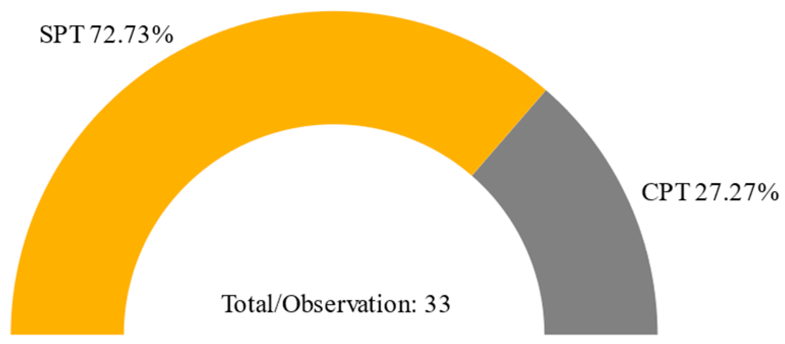
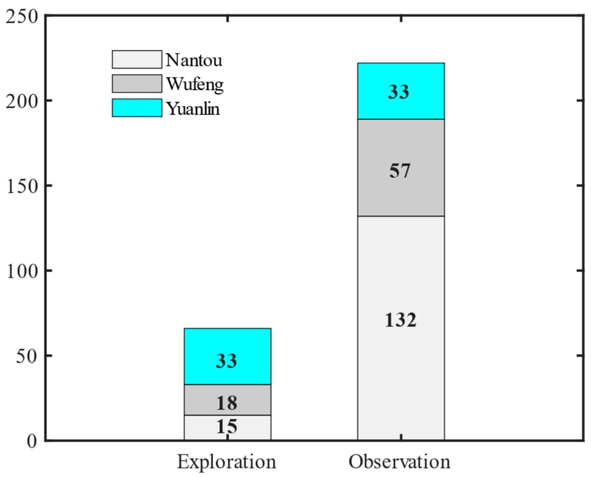
For the target region of this study, the number of directly observable points is significantly larger than that of the exploration points with test data, and all these data are sourced from the Next Generation Liquefaction (NGL) project [44] which has been developed for researchers to access liquefaction case history data shared by other researchers, and to share their own data in return. Among the exploration points, those obtained through the Standard Penetration Test (SPT) constitute a relatively large proportion, while the number of exploration points acquired by other geotechnical investigation methods is relatively small. An overview of data types related to soil liquefaction is presented in

Table 1. Liquefaction data overview.

Region	Exploration Points SPT/Others	Observation Points	Total
Nantou	9/6	132	132
Wufeng	14/4	57	57
Yuanlin	24/9	33	33

, Figure 2 and Figure 3 below. These differences in the quantity of points from various sources highlight the challenges and limitations in comprehensively assessing the geotechnical conditions of the region.

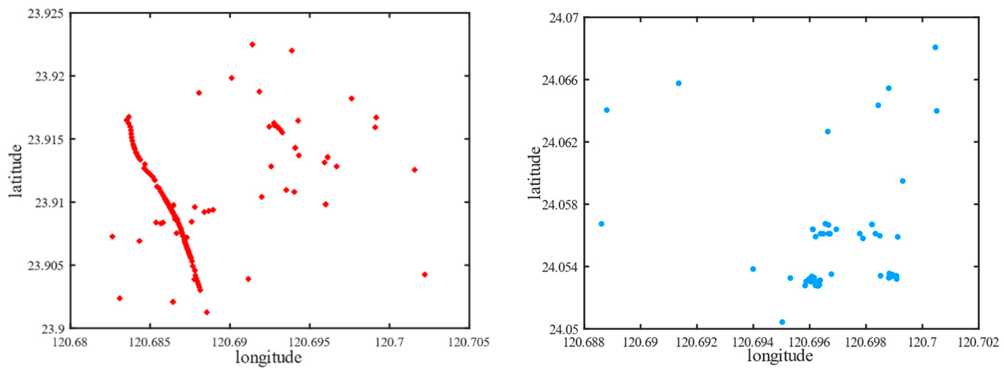
In addition to the sparse nature of the available data, the observed points are highly concentrated in specific locations while being extremely scarce in other areas, as shown in Figure 4. This uneven distribution hinders accurate liquefaction assessment for the entire region. Moreover, severe unevenness can exaggerate apparent trends, which often deviate from reality when data are sparse or uncertainties are high. Additionally, the scarcity in other locations can significantly affect the overall regional liquefaction assessment, undermining its accuracy and representativeness due to insufficient spatial coverage.

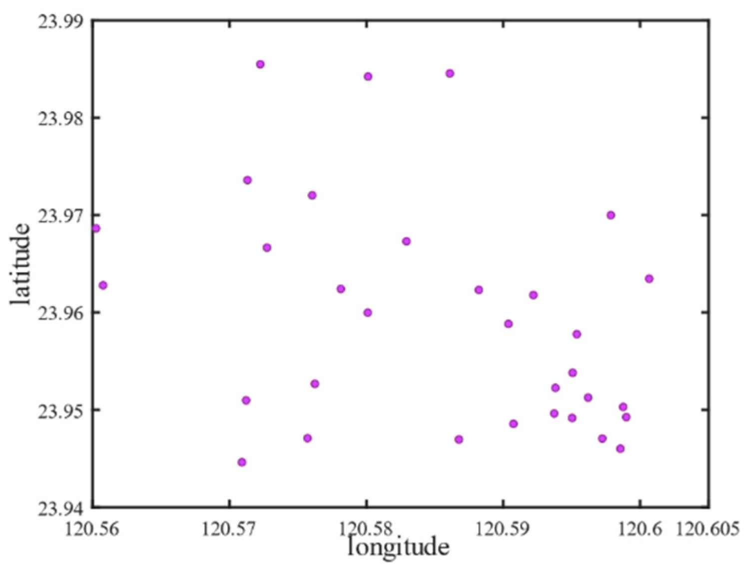
Among the three regions, the points in Yuanlin are more evenly distributed within the study area. There is no significant concentration or scarcity of points in specific locations, as illustrated in Figure 5. Considering this advantageous distribution pattern, which can provide more comprehensive and representative data for the liquefaction assessment, Yuanlin during this earthquake event is selected as the object of study for the target region.

2.3. Distribution of Seismic Ground Motion Intensity

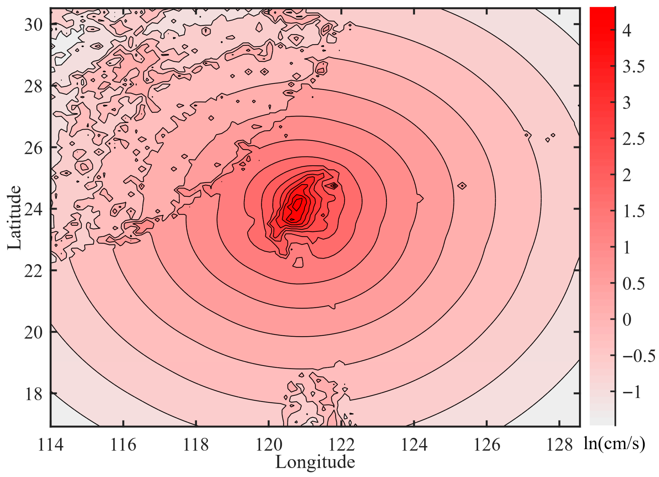
The ground motion intensity distribution map for the 1999 Chi-Chi earthquake event is obtained from ShakeMap. Peak ground velocity (PGV) is selected as the ground motion intensity measure [45]. The distribution map is shown in Figure 6 below. It should be noted that this study exclusively employs PGV as the seismic intensity measure, while incorporating additional ground motion intensity measures (e.g., peak ground acceleration) could be considered for enhanced characterization.

3. Rapid Assessment Procedure of Regional Probabilistic Liquefaction Based on Transfer Learning

3.1. Conditions for Rapid Assessment of Regional Seismic Liquefaction

3.1.1. Limitations of Liquefaction Data

The objective of this study is to rapidly assess the regional probabilistic liquefaction during a specific earthquake event when liquefaction has already occurred after the earthquake, or to evaluate the regional probabilistic liquefaction under the scenario earthquake. This assessment aims to provide a basis for subsequent loss evaluation, functional recovery, and resilience enhancement.

Earthquakes generally affect a large-scale area. However, it is extremely difficult to obtain extensive stratigraphic exploration data. The larger the regional scope, the more challenging it is to overcome such difficulties. Surveys immediately after an earthquake can often quickly acquire direct seismic liquefaction information. Nevertheless, the direct liquefaction information obtained from surveys is usually rather rough, lacking soil layers conditions and exploration data. Figure 7 also reflects the scarcity of exploration data, while the observational data from post-earthquake surveys are relatively abundant. Meanwhile, following an earthquake, the stratum conditions in the earthquake-affected area will be substantially influenced. Particularly in regions where liquefaction has occurred, the stratum state will differ from its condition prior to the earthquake. Later supplementary explorations cannot fully represent the pre-earthquake stratum conditions. It is essential to conduct rapid seismic liquefaction assessments over a regional scale, both in terms of time and space.

3.1.2. Seismic Information

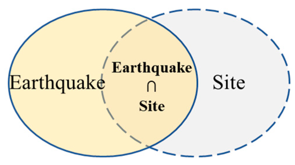
Benefiting from the current research achievements in seismology and earthquake engineering [46,47,48,49], it is possible to analyze the regional distribution of seismic ground motion intensity relatively quickly by utilizing the existing data from seismic stations and stratigraphic data after an earthquake. Studies on the site seismic response have also demonstrated the significant influence of geological conditions such as the properties of the strata, topography, and geomorphology on the propagation of seismic waves [50,51,52,53,54]. The influence of stratigraphic conditions is also considered in the seismic ground motion prediction equations, indicating that the seismic ground motion information inherently contains stratigraphic information. In the authors’ work on the global importance analysis of the prediction factors for the probability of liquefaction, it has also been verified that the influence of seismic load on the liquefaction probability includes the cross terms of stratigraphic conditions, as illustrated in Figure 8.

In fact, given the site conditions, liquefaction probability is a conditional probability function of ground motion intensity, as demonstrated in Equation (1) [45]. Therefore, leveraging the seismic ground motion information comprehensively and integrating it with the post-earthquake on-site liquefaction surveys can provide the essential basis for the rapid assessment of regional seismic liquefaction.

$$F_{\mathrm{R}}(\mathrm{LS}|\mathrm{IM}=x)=\mathsf{\Phi }\left({\displaystyle \frac{\ln (x/\theta )}{\beta }}\right)$$

(1)

where F_R( ) is the liquefaction fragility function of ground motion intensity, LS is the liquefaction state, IM represents the intensity measure of ground motion, Φ( ) is the standard normal cumulative probability function, θ denotes the median value of the distribution, and β denotes the logarithmic standard deviation.

3.1.3. Feasibility of Rapid Regional Liquefaction Assessment

Seismic liquefaction correlates with both seismic parameters and site characteristics, with all existing assessment methods relying on these two categories of data. However, as previously analyzed, the scarcity of subsurface exploration data in practice imposes significant limitations on large-scale regional liquefaction assessments. Even existing machine learning models struggle to operate effectively in the absence of critical soil property parameters. In contrast to site exploration data, seismic information and liquefaction observations can be acquired more rapidly and conveniently. As demonstrated in Section 3.1.2, seismic information not only has a direct correlation with liquefaction but also implicitly contains certain site-specific attributes, rendering it plausible to conduct rapid regional liquefaction assessments using only seismic data and liquefaction observations.

Notably, excluding site exploration data inherently introduces varying degrees of distortion into liquefaction assessments. To mitigate this limitation, this study constrains its scope to a specific region affected by a single seismic liquefaction event, under the premise of widespread liquefaction occurrences. In accordance with Section 2.2, Yuanlin City is selected as the study region.

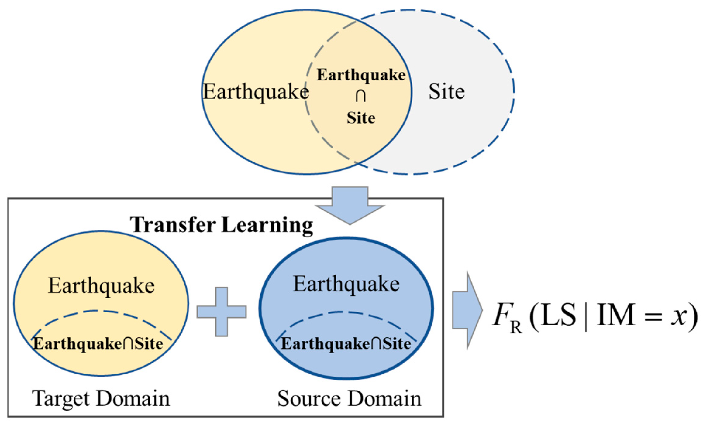
The dual constraints of focusing on a single liquefaction event and relying solely on seismic and observation data inevitably lead to insufficient data volume and information gaps. To address this, transfer learning is employed to overcome data sparsity and supplement domain knowledge. As illustrated in Figure 9, transfer learning enables the transfer of knowledge or experience derived from a source domain to a target domain, thereby addressing challenges associated with target-domain data scarcity and model training complexities, and enabling the achievement of the study’s objectives.

3.2. Feature-Based Transfer Learning

The rapid assessment procedure for regional probabilistic liquefaction proposed in this study adopts a feature-based transfer learning approach. Transfer learning involves applying the knowledge acquired from source domain to target domain, thereby enhancing the performance and generalization ability of the model. For the framework proposed in this paper, the prerequisite is to construct a source domain that contains rich and complete information. The core of this framework is to learn the domain-invariant and discriminative features between the source domain and the target domain. Furthermore, it aims to achieve the predefined task objectives in the target domain where both the data and parameters are limited.

3.2.1. Transfer Learning Architecture

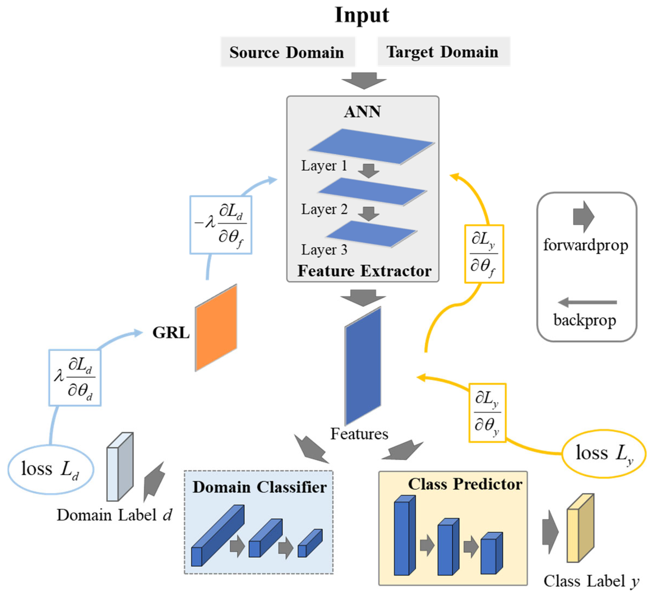
A feature-based transfer learning method, namely the Domain-Adversarial Neural Network (DANN), is employed. The introduced architecture consists of a deep feature extractor, a deep class predictor, a domain classifier, and a gradient reversal layer. An artificial neural network (ANN) is employed as the feature extractor to construct a Domain-Adversarial Neural Network (DANN), as illustrated in Figure 10. The description of loss propagation in Figure 10 is provided in Section 3.2.2. The feature extractor is designed to extract high-level features from the input data. These features are then used for the primary task, such as classification, as well as for domain adaptation. Domain adaptation is achieved by incorporating a domain classifier that is linked to the feature extractor through the gradient reversal layer (GRL). The function of this domain classifier is to determine whether the extracted features originate from the source domain or the target domain.

The GRL is a crucial component in the DANN. In domain adaptation, the aim is to allow models to transfer source domain knowledge to the target domain. The GRL’s core concept is to achieve similar feature distributions between the source and target domains for the features extracted by the feature extractor via adversarial training. As a unique network layer, the GRL keeps the input data intact during forward propagation and multiplies the gradient by a negative constant λ during backpropagation.

3.2.2. Domain-Invariant and Discriminative Feature Training

The DANN model serves as an advanced extension of the traditional feed-forward neural network, endowing it with enhanced capabilities for handling domain adaptation tasks. It is amenable to training using the majority of stochastic gradient descent-based optimization algorithms.

Let $D_f\left({\mathit{x}}_i;{\theta }_f\right)$ denote an artificial neural network feature extractor parameterized by ${\theta }_f$, where x_i represents the input data and the feature extractor D_f maps the input data x_i into a feature space. Also, let $D_d\left({\mathit{x}}_i;{\theta }_d\right)$ represent the output of domain prediction with ${\theta }_d$ as the parameter, while $D_y\left({\mathit{x}}_i;{\theta }_y\right)$ now corresponds to the computation of the network’s label prediction output layer, with parameters ${\theta }_y$. The classification prediction loss and the domain loss are, respectively, as follows:

$$L_y^i\left({\theta }_f,{\theta }_y\right)=L_y\left(D_y\left(D_f\left({\mathit{x}}_i;{\theta }_f\right);{\theta }_y\right),y_i\right)$$

(2)

$$L_d^i\left({\theta }_f,{\theta }_d\right)=L_d\left(D_d\left(D_f\left({\mathit{x}}_i;{\theta }_f\right);{\theta }_d\right),d_i\right)$$

(3)

According to the research [55], the corresponding parameters of the DANN model are derived by finding the stationary points through the following gradient update equations:

$${\theta }_f-r\left({\displaystyle \frac{𝜕L_y^i}{𝜕{\theta }_f}}-\lambda {\displaystyle \frac{𝜕L_d^i}{𝜕{\theta }_f}}\right)\to {\theta }_f$$

(4)

$${\theta }_y-r{\displaystyle \frac{𝜕L_y^i}{𝜕{\theta }_y}}\to {\theta }_y$$

(5)

$${\theta }_d-r\lambda {\displaystyle \frac{𝜕L_d^i}{𝜕{\theta }_d}}\to {\theta }_d$$

(6)

The parameters mentioned above can be obtained through the gradient descent realized via the gradient reversal layer (GRL) [55]. The GRL is a layer devoid of any associated parameters. Specifically, in the process of forward propagation, it acts as an identity transformation. Conversely, during backpropagation, the GRL retrieves the gradient from the subsequent layer, changes its sign by multiplying it with −1, and then passes it to the preceding layer. Implementing this layer only requires defining the procedures for forward propagation (which is an identity transformation) and backpropagation (where the gradient is multiplied by −1). As previously defined, the GRL is inserted between the feature extractor $D_f$ and the domain classifier $D_d$, resulting in the architecture depicted in Figure 10. Mathematically, the GRL can be represented as a function $G\left(x\right)$. This function is defined by two specific equations that are distinct and mutually exclusive, which, respectively, describe its behavior during forward propagation and backpropagation:

$$G\left(x\right)=x$$

(7)

$${\displaystyle \frac{dG}{dx}}=-\mathrm{I}$$

(8)

where $\mathrm{I}$ is the identity matrix. The parameter sets $\left({\theta }_f,{\theta }_y,{\theta }_d\right)$ are being optimized through stochastic gradient descent in the method [55]:

$$\begin{array}{l}E\left({\theta }_f,{\theta }_y,{\theta }_d\right)={\displaystyle \frac{1}{n}}{\displaystyle {\displaystyle \sum _{i=1}^n}{L}_y\left(D_y\left(D_f\left({\mathit{x}}_i;{\theta }_f\right);{\theta }_y\right),y_i\right)}\\ -\lambda \left({\displaystyle \frac{1}{n}}{\displaystyle {\displaystyle \sum _{i=1}^n}{L}_d}\left(D_d\left(G\left(D_f\left({\mathit{x}}_i;{\theta }_f\right)\right);{\theta }_d\right),d_i\right)+{\displaystyle \frac{1}{n^{\prime }}}{\displaystyle {\displaystyle \sum _{i=n+1}^N}{L}_d\left(D_d\left(G\left(D_f\left({\mathit{x}}_i;{\theta }_f\right)\right);{\theta }_d\right),d_i\right)}\right)\end{array}$$

(9)

By performing gradient descent on Equation (9), the model parameters can be optimized. This process not only facilitates the overall optimization of the model but also results in the generation of features that are simultaneously domain-invariant and discriminative.

In the work, the model construction, training, and parameter optimization are all implemented using the PyTorch framework in Python.

3.2.3. Dataset Construction

Source Domain Dataset

To address the issues of sparsity and imbalance in the actual data, in the present study, the source domain dataset is generated via probability modeling of the site conditions and finite element calculations with the aid of OpenSees. Statistical and probabilistic modeling of liquefaction cases from the literature [56,57] form the basis for this analysis with primary considerations including groundwater table depth, sand layer thickness, burial depth of sand layers, and sand layer relative density.

• Burial depth of sand layers: The burial depth of sand layers is found to follow a log-normal distribution with parameters θ = 1.62 and β = 0.7596. This distribution is validated through a Kolmogorov–Smirnov (KS) test at a significance level of 0.05.
• Groundwater level: Analysis of groundwater-level probability distributions from sample library A reveals that the log-normal distribution is appropriate, as verified by a KS test at a significance level of 0.01. To improve statistical robustness, three outliers are removed, as their exclusion does not affect the overall sample range. The refined groundwater-level data follow a log-normal distribution with parameters θ = 0.299 and β = 0.6856, passing the KS test at a significance level of 0.05.
• Sand layer thickness: The thickness of the sand layer follows a log-normal distribution with parameters θ = 0.4071 and β = 0.7053, which is validated through the KS test at a significance level of 0.05.

In comparison to actual liquefaction cases, the construction of the source domain dataset allows for a more comprehensive selection of ground motions. To mitigate potential biases in the results due to the choice of ground motions, this study selects representative ground motion records based on the Mw-R classification. A total of 314 ground motion records is selected from the PEER database to form the earthquake motion database for this study. The distribution of Mw-R in the selected seismic motion records is shown in Figure 11. In this study, both R and R-rup denote epicentral distance.

In order to reduce the number of calculations and ensure that the collected samples are evenly distributed across the variable distribution range, an improved Latin hypercube sampling method is adopted in this analysis to sample the site condition variables 200 times [58].

This analysis requires only 200 Latin hypercube samplings of the site conditions. Considering three scenarios of loose sand, moderately dense sand, and dense sand, each scenario corresponds to 200 site conditions. For each site, 314 selected ground motions are input for seismic liquefaction calculations to obtain the results of liquefaction occurrence and non-occurrence. Finally, a seismic liquefaction source domain dataset containing 188,400 samples is constructed, as shown in

Table 2. Source domain dataset summary.

Database	Size	Size (Liquefied)	Proportion (Liquefied)	Range
Source domain	188,400	47,581	25.3%	Sand layer depth 0.70~17.33 m
				Groundwater level 0.21~4.13 m
				Sand layer thickness 0.20~4.65 m

.

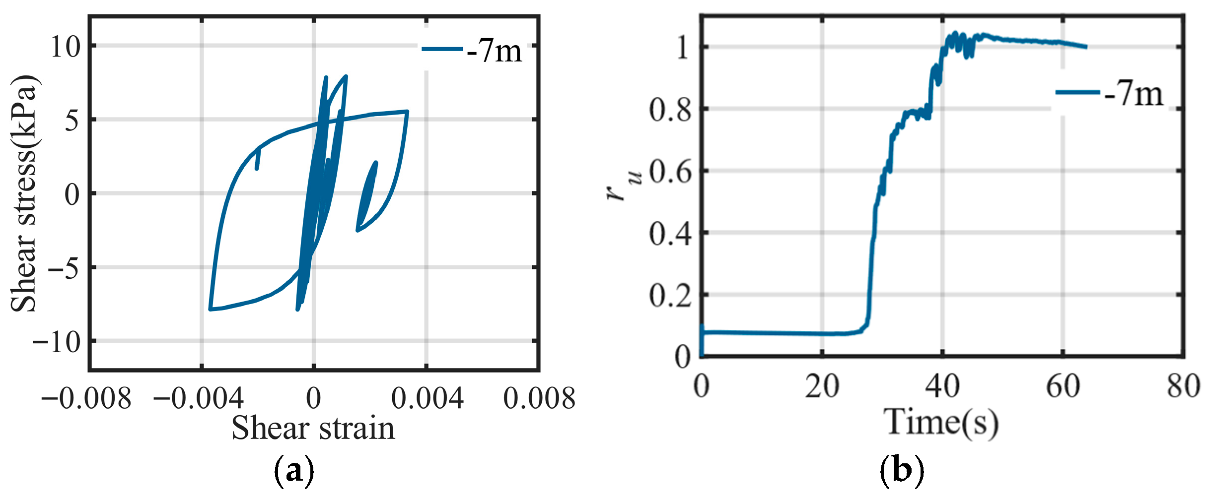
The liquefaction behavior at a representative site was analyzed through numerical simulation under seismic loading conditions, with particular attention to the 7 m-depth stratum. The simulation results demonstrate characteristic liquefaction phenomena, including nonlinear stress–strain response and progressive development of excess pore water pressure ratio (r_u). As shown in Figure 12, complete liquefaction occurred when the excess pore water pressure ratio reached unity during ground motion, indicating full loss of soil shear strength.

Target Domain Dataset

The target domain dataset consists of the seismic liquefaction data from the Chi-Chi earthquake event which is the focus of this study. Since the target area is Yuanlin during this earthquake event, the seismic liquefaction data from Nantou and Wufeng within the target domain dataset are designated as the target domain training set, while the seismic liquefaction data from Yuanlin are used as the target domain test set or prediction set.

In this way, in terms of the geographical dimension, the data sources of the prediction set and the training set are different. They are from different regions within the same seismic liquefaction event. Moreover, this approach can overcome the challenge of limited data in Yuanlin. All the above measures contribute to making the model’s prediction of seismic liquefaction in Yuanlin more reliable.

Model Parameters

Based on the conditions described in Section 3.1, the model parameters selected in this study mainly include seismic ground motion-related parameters and the liquefaction results observed from on-site surveys. The seismic ground motion-related parameters encompass the magnitude of the earthquake (M_w), the epicentral distance (R), and the intensity of the seismic ground motion (PGV). It should be noted that the rapid assessment procedure for regional probabilistic liquefaction proposed in this paper is also constrained by the shortage of exploration data. Incorporating the uncertainties of soil property parameters and spatial correlations in future research may lead to more favorable results.

3.3. Rapid Assessment Procedure of Regional Probabilistic Liquefaction Based on Transfer Learning

The rapid assessment of the liquefaction probability in a specific region depends on the timely acquisition of seismic information. In contrast to detailed geological exploration data, seismic information can generally be obtained promptly. Although it has been elaborated in Section 3.1 that seismic ground motion information encompasses certain site information, in the current research landscape, relying merely on seismic information for liquefaction assessment is unlikely to yield satisfactory outcomes. Therefore, in this work, by using a transfer learning framework, we employ the source domain dataset that is rich in seismic and site information. This approach helps to overcome the limitations of conducting liquefaction assessment in the target region when relying only on seismic information, thus making rapid liquefaction assessment possible. The procedure for rapid regional liquefaction probability assessment is illustrated in Figure 13, and it mainly comprises the following key components:

(a)

Establishment of the Target Domain Dataset: For this component, the liquefaction data from the Chi-Chi earthquake event are chosen as the target domain. This target domain encompasses three regions: Wufeng, Nantou, and Yuanlin, with Yuanlin being designated as the research object.

(b)

Construction of the Source Domain Dataset: When it comes to constructing the source domain dataset, data-driven approaches are employed to generate site conditions that are rich enough. After conducting the modeling process with OpenSees, we input a substantial number of actual ground motions. Subsequently, through the seismic liquefaction response analysis, a source domain dataset that is abundant in both seismic information and site information is acquired.

(c)

Transfer Learning-based Model Training across Source and Target Domains: In the process of training a model across the source and target domains based on transfer learning, we leverage the data from both these domains. Through transfer learning techniques, a seismic liquefaction assessment model is trained. This model primarily relies on the ground motion information and the post-earthquake liquefaction survey data of the region.

(d)

Regional Liquefaction Probability Assessment: To evaluate the liquefaction probability of the target region, we utilize the transfer learning model established in component (c) along with the seismic information specific to the target region.

Figure 13. Rapid assessment procedure of regional probabilistic liquefaction based on transfer learning.

Figure 13. Rapid assessment procedure of regional probabilistic liquefaction based on transfer learning.

4. Liquefaction Probability Assessment of the Target Region

In this section, the previously described rapid assessment procedure is employed to conduct a liquefaction assessment of the target area. Additionally, a performance comparison of relevant models is carried out, and a distribution map for the assessment of the liquefaction probability in the target area will be presented.

4.1. Model Training Schemes

To evaluate the performance of the proposed rapid liquefaction assessment procedure relying exclusively on seismic information and liquefaction observation data, this subsection presents experimental designs to compare it with models that integrate seismic information, site-specific data, and liquefaction observations concurrently. Furthermore, an Artificial Neural Network (ANN) model is incorporated into the comparative framework based on the above analyses. Owing to divergent data dependency profiles, both the dataset scales and input parameters utilized for training and evaluating model performance exhibit variations across different methodologies.

The primary objective is liquefaction assessment in Yuanlin, where liquefaction data from Yuanlin constitute the test set, while data from Nantou and Wufeng serve as the training set. For site-dependent models, SPT measurements are selected as model parameters due to their relative abundance, resulting in a curated dataset smaller than the total available borehole records.

Table 3. Summary of model training schemes.

Scheme	Model	Train Size	Test Size	Earthquake-Related Parameters	Site-Related Parameters	Notes
1	DANN	Nantou, Wufeng 189	Yuanlin 33	√	×	Rapid Assessment Procedure
2	ANN	Nantou, Wufeng 189	Yuanlin 33	√	×	-
3	DANN	Nantou, Wufeng 23	Yuanlin 24	√	√	-
4	ANN	Nantou, Wufeng 23	Yuanlin 24	√	√	-

summarizes the comparative training schemes.

Site-related parameters primarily include three vertical depths in the sand layer and their corresponding SPT blow counts (N1, D1, N2, D2, N3, D3), as well as the groundwater table depth (DW).

4.2. Model Performance Evaluation

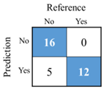
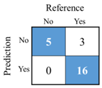
The primary metric for assessing model performance is overall accuracy, which directly reflects whether the model meets the task requirements. Accuracy represents the proportion of correctly predicted samples to the total number of samples and serves as the most intuitive indicator for evaluating a model’s overall performance. Furthermore, the Kappa coefficient is selected as a complementary metric to deal with the difficulties presented by the skewed distribution of positive and negative samples. The Kappa coefficient ranges from −1 to 1, where 1 indicates perfect classification or complete agreement, 0 corresponds to classification equivalent to random guessing, and negative values signify performance worse than random guessing (a rare occurrence in practice). Most of these indicators can be derived from the confusion matrix (CM), which summarizes the statistical outcomes of classification tasks. The confusion matrix includes the following components: true positive (TP), true negative (TN), false positive (FP), and false negative (FN).

Table 4. The structure of the confusion matrix.

		Reference
		No	Yes
Prediction	No	TN	FN
	Yes	FP	TP

below illustrates the structure of the confusion matrix.

The calculation of performance indicators is as follows:

• Accuracy:

$$OA={\displaystyle \frac{TN+TP}{TN+FN+TP+FP}}$$

(10)

• Kappa:

$$K={\displaystyle \frac{OA-RA}{1-RA}}$$

(11)

where RA denotes the random or predictive accuracy, as defined below:

$$RA={\displaystyle \frac{(TP+FP)(TP+FN)+(FN+TN)(FP+TN)}{{(TP+FP+FN+TN)}^2}}$$

(12)

The DANN model in Scheme 1 is trained according to the rapid assessment procedure of regional probabilistic liquefaction based on transfer learning described in Section 3. The training results and performance are presented in

Table 5. Model training results and performance with earthquake-related parameters.

Scheme	Model	Model Parameters	Confusion Matrix	Performance
1	DANN	lnMw, R, PGV		Accuracy: 0.849 Kappa: 0.700
2	ANN	lnMw, R, PGV		Accuracy: 0.697 Kappa: 0.380

. For comparative analysis, the training outcomes of Scheme 2, Scheme 3 and Scheme 4 are listed in Table 5 and

Table 6. Model training results and performance with earthquake-related parameters and site-related parameters.

Scheme	Model	Model Parameters	Confusion Matrix	Performance
3	DANN	lnMw, R, PGV N1, D1, N2, D2, N3, D3, DW		Accuracy: 0.875 Kappa: 0.690
4	ANN	lnMw, R, PGV N1, D1, N2, D2, N3, D3, DW		Accuracy: 0.750 Kappa: 0.308

.

In Scheme 2, the ANN model relying solely on earthquake-related parameters exhibited significantly lower accuracy and Kappa coefficient than the DANN model in Scheme 1, particularly for the Kappa coefficient. The DANN model in Scheme 3 incorporated both earthquake-related and site-related parameters. However, due to the scarcity of exploration data compared to observational data in practice, its accuracy is only marginally higher than that of the earthquake-only DANN model in Scheme 1, with no improvement in the Kappa coefficient. The ANN model in Scheme 4 also demonstrated conspicuously inferior performance to the DANN model in Scheme 1.

Overall, the proposed rapid liquefaction assessment method (DANN model in Scheme 1), relying exclusively on seismic parameters and liquefaction observations without site-specific data, demonstrates performance comparable to the site-inclusive DANN model and significantly outperforms ANN models (both those with and without site data). Crucially, its input parameters enable more rapid, economical acquisition, rendering it particularly suitable for large-scale regional rapid liquefaction assessments.

The rapid regional liquefaction assessment procedure proposed in this paper demonstrates good performance, and there are challenges in large-scale acquisition of site-related parameters for all locations within the target region. In the subsequent parts of this paper, the research will predominantly be carried out based on the DANN model in Scheme 1.

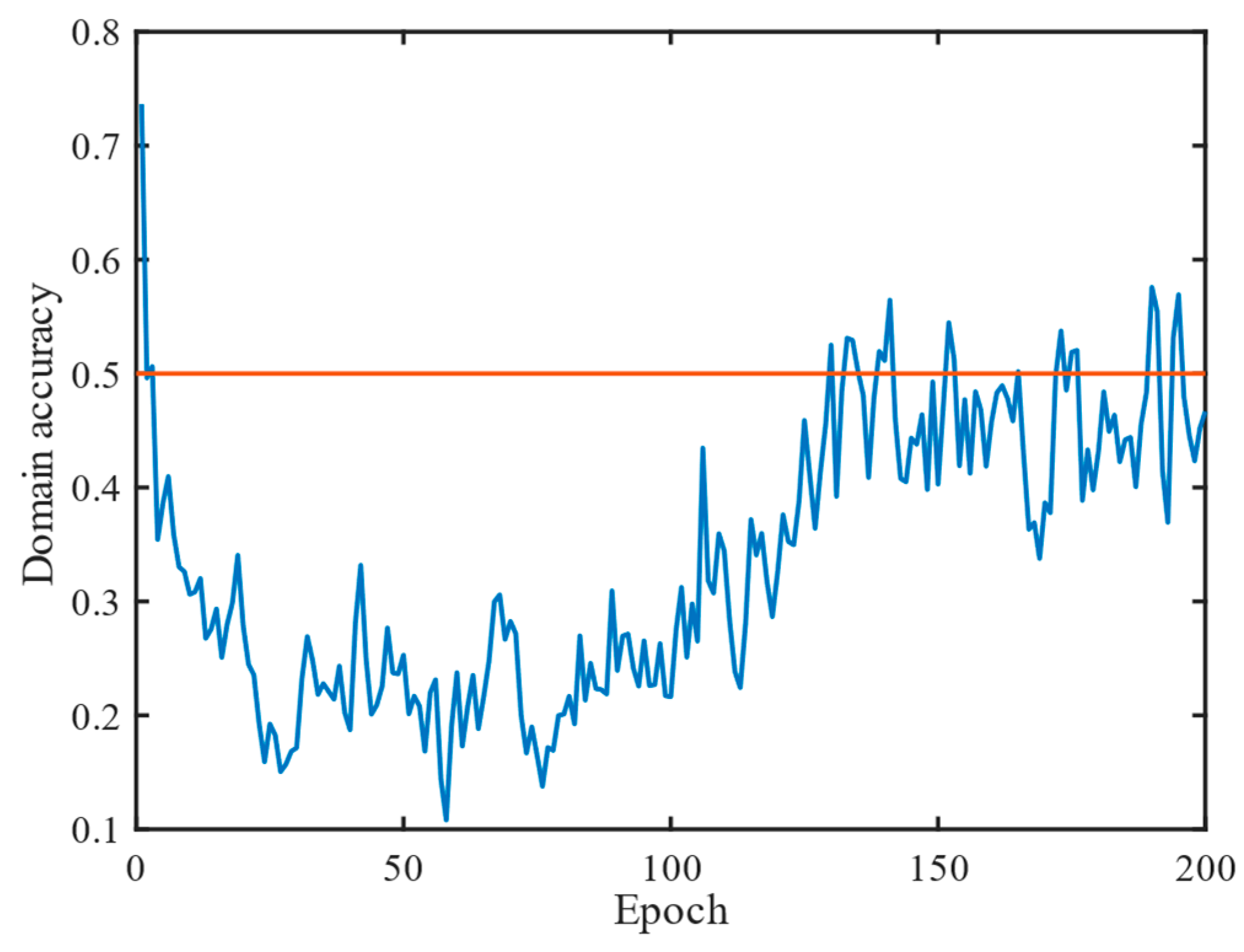
The domain adaptation process incorporates explicit monitoring of feature space alignment through the domain classifier accuracy (Figure 14). As training progresses, the domain classification accuracy approaching 0.5 indicates successful domain-invariant feature learning, where the model can no longer reliably distinguish between source and target domains.

In Scheme 1, the seismic input parameters are limited to M_w, R, and PGV. While PGV can be derived from ground motion prediction equations (GMPEs), other earthquake descriptors such as frequency content or duration may further refine liquefaction potential estimation. However, parameters like frequency and duration are typically only available at seismic station locations, and current methodologies lack reliable approaches to extrapolate these spatially across unsampled regions. Future advances in dense instrumentation or physics-based ground motion synthesis may enable the incorporation of such features.

4.3. Liquefaction Probability Assessment of the Target Region

When conducting a binary classification task, the transfer learning model utilizes the sigmoid function to derive the corresponding class probabilities, based on which the classification judgment is subsequently made. The sigmoid function is presented in Equation (13).

$$P(y=1\left|\mathit{x}\right.)={\displaystyle \frac{1}{1+e^{-(w^T\mathit{x}+b)}}}$$

(13)

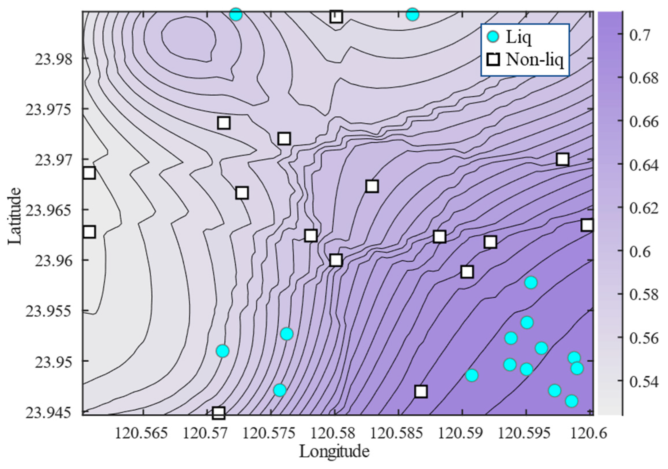
In this study, the class prediction output of the transfer learning model is taken as the value of the sigmoid function, which serves as the class probability. Subsequently, the liquefaction probability distribution of Yuanlin is obtained, as illustrated in Figure 15. The solid cyan circles represent the identified liquefaction points, while the hollow squares represent the sampled points where no liquefaction occurred.

According to the liquefaction probability distribution map in Figure 8, the area in the lower right corner of Yuanlin is the most prone to liquefaction. In fact, the majority of the identified liquefaction occurrences are found in this region.

5. Regional Liquefaction Probability Index

In the previous section, an analysis is conducted on the assessment of the regional liquefaction probability, and a liquefaction probability distribution map was provided, which allows for an intuitive visualization of the overall distribution of liquefaction probabilities in Yuanlin City. However, the analysis lacks an overall index for evaluating the probability of liquefaction within the region. This section presents the assessment index for regional probabilistic liquefaction and its applications.

5.1. Definition and Formula of the Regional Liquefaction Probability Index

Considering the uncertainties of ground motion, even for the same site underground motions of the same intensity but with different characteristics, there may still be two possible scenarios: liquefaction and non-liquefaction. Under specified site conditions, liquefaction probability can be modeled as a conditional probability function of ground motion intensity [45]. Representing the liquefaction situation with the liquefaction probability is a more accurate approach.

In regional probabilistic liquefaction assessment, this study proposes using the average liquefaction probability per unit area as the assessment index. The specific calculation method, defined herein, involves dividing the integral of liquefaction probability over the regional area by its total area, as shown in the following formula:

$$L_{\mathrm{region}}={\displaystyle \frac{{\displaystyle {\iint }_{D}P(x,y)dA}}{D}}={\displaystyle \frac{{\displaystyle {\iint }_{D}P(x,y)dxdy}}{D}}\approx {\displaystyle \frac{{\displaystyle {\sum }_{i=1}^m{\displaystyle {\sum }_{j=1}^{n}P({\xi }_i,{\eta }_j)∆A_{ij}}}}{{\displaystyle {\sum }_{i=1}^m{\displaystyle {\sum }_{j=1}^n∆A_{ij}}}}}$$

(14)

where $P(x,y)$ represents the liquefaction probability function with respect to the coordinates $(x,y)$; $P({\xi }_i,{\eta }_j)$ denotes the liquefaction probability of the representative point $({\xi }_i,{\eta }_j)$ in the area $(i,j)$.

Based on the definition and the significance, the value of the regional liquefaction probability index lies between 0 and 1. The closer the value is to 1, the higher the regional liquefaction probability is, signifying a greater propensity for liquefaction to occur. Conversely, a lower value implies a lower regional liquefaction probability. The relationship between the index and the consequences of liquefaction disasters is not considered for now.

It should be noted that this index can automatically adapt to regional liquefaction assessments for regions of varying sizes and enables comparisons under uniform conditions. In this study, the proposed regional liquefaction probability index quantifies the central tendency of liquefaction probability based on the trained model’s predictions. While the current framework does not explicitly incorporate uncertainty analysis (e.g., data variability, model parameter sensitivity, or sampling errors) needed to derive formal confidence intervals, we recognize their importance in assessing the index’s reliability and spatial variability. Future work will prioritize integrating uncertainty quantification methods to calculate confidence intervals, thereby enhancing the robustness of the index mapping and supporting more informed decision-making in practical applications.

5.2. Applications of the Regional Liquefaction Probability Index

5.2.1. Application Based on Transfer Learning

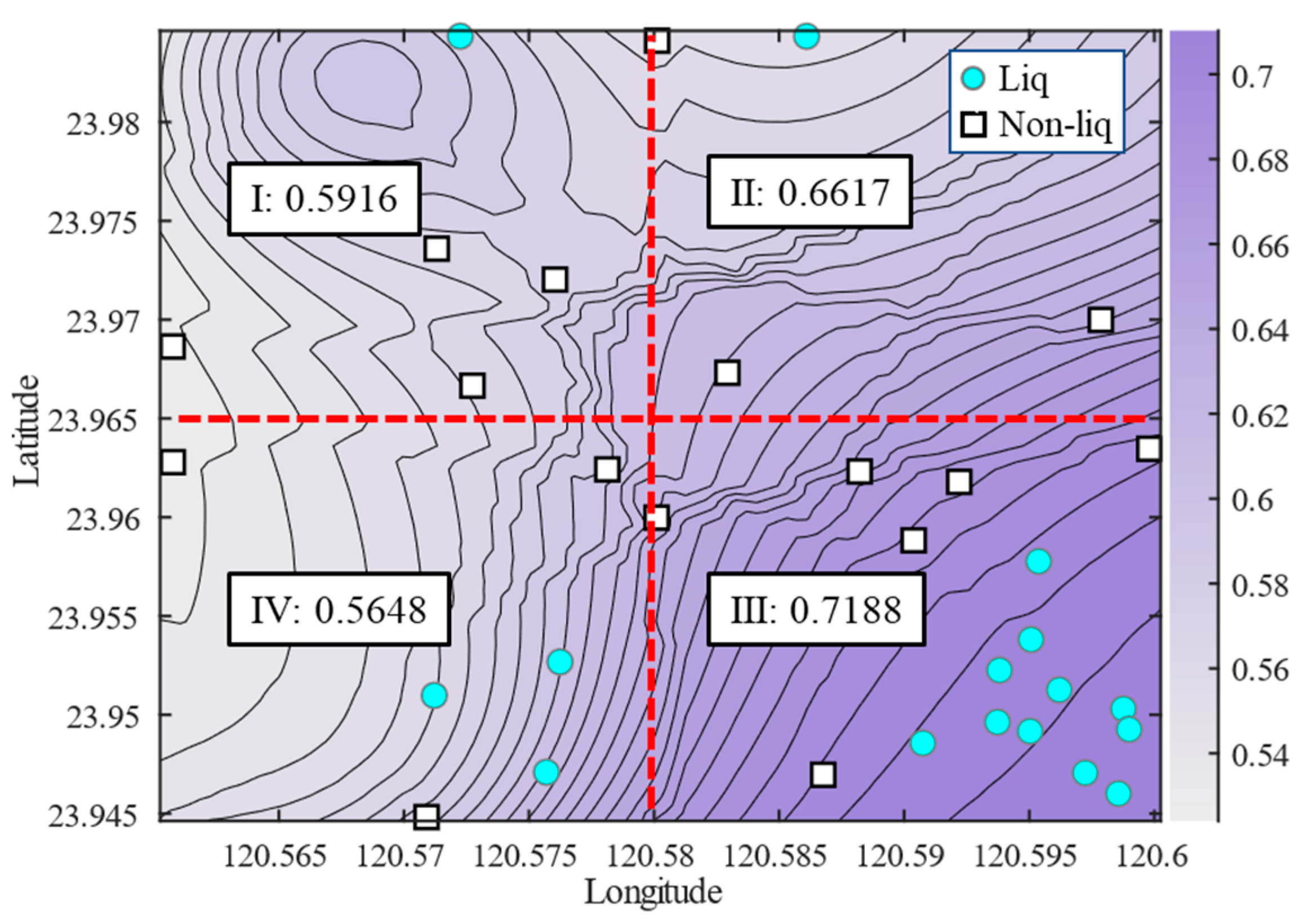
Based on the content of Section 4, this part calculates the regional liquefaction probability index of the target region. The Yuanlin area is divided equally into four parts, and the regional liquefaction index of each part is calculated separately. The results of the division and calculation are shown in Figure 16 below.

The area with the highest index is Area Ⅲ, followed by Area Ⅱ, which is consistent with the results visually observed from the liquefaction probability distribution map. However, the results provided by the liquefaction probability distribution map are qualitative and based on subjective observations. In situations where it is impossible to make an obvious and direct distinction, it is difficult to conduct comparisons. Moreover, it is challenging to quantify subjective and qualitative results. By using the regional liquefaction probability index, we can directly compare the overall liquefaction potential of different regions and obtain a quantitative result, which provides a basis for subsequent assessment of regional liquefaction losses, functional recovery, and enhancement of resilience.

5.2.2. Simplified Application

In this subsection, a simplified calculation method of the regional liquefaction probability index is presented. This method relies on the distribution of the survey points in the target region after the earthquake. Ideally, the points should be evenly and densely distributed. Take Yuanlin as an example again. It should be noted that the post-earthquake survey points in Yuanlin are relatively evenly and densely distributed only in Area III, while the distribution in the remaining areas is relatively sparse. The calculation results are mainly intended to illustrate the calculation method and do not represent the accuracy of the results.

According to the post-earthquake survey results, for the points where liquefaction occurred, their liquefaction probability is set to 1, while for those points without observed liquefaction phenomena, the liquefaction probability is set to 0. Then, the inverse distance spatial interpolation method is employed to conduct spatial interpolation of the liquefaction probability, thus obtaining the liquefaction probability at any location. Based on this, the regional liquefaction probability index is calculated. The calculation results are presented in Figure 17 below.

As shown in Figure 17, the results obtained by the simplified calculation method indicate that Area Ⅲ has the highest index, which is consistent with the conclusions drawn from the liquefaction probability distribution map and those in Section 5.2.1. However, the simplified method is unable to consider the uncertainties of liquefaction. The observation points in the remaining areas are too sparse to draw reliable conclusions. During post-earthquake surveys, the reliability of the simplified method can be improved by arranging observation points evenly and densely, which is both feasible and relatively easy to implement.

6. Conclusions

This study presents a rapid assessment procedure for regional probabilistic liquefaction using transfer learning. The procedure leverages seismic data from liquefaction events and post-earthquake observation points to enable efficient liquefaction assessment. A novel regional liquefaction probability index is introduced, and both the procedure and index are demonstrated through their application to the Chi-Chi earthquake case, illustrating practical utility. The main conclusions are as follows:

(1)

A rapid assessment procedure of regional probabilistic liquefaction based on transfer learning is proposed in this study (DANN model in Scheme 1), which relies solely on earthquake information and liquefaction observations in the absence of site-related data. It exhibits performance comparable to the site-incorporating DANN model and significantly outperforms all ANN models, regardless of site data inclusion. Additionally, its model parameters can be acquired more quickly, conveniently, and at lower cost, making it suitable for large-scale regional liquefaction assessments.

(2)

Regional liquefaction probability assessment for Yuanlin reveals that the southeastern area is the most prone to liquefaction. This finding matches post-earthquake survey results, where actual liquefaction instances are predominantly concentrated in this region.

(3)

The proposed regional liquefaction probability index, when applied to Yuanlin, identifies the southeastern area as having the highest index values, consistent with both the regional probabilistic liquefaction distribution and observed liquefaction patterns. A simplified calculation method for the index is provided, which depends on the distribution and density of post-earthquake observation points, ensuring strong practical applicability.

(4)

The developed procedure and index rely principally on the uniformity of post-earthquake liquefaction observation point distribution and their density, offering notable advantages in real-world applications, including high efficiency, low cost, and strong implementability.

Limitations: Due to the challenges in acquiring large-scale site exploration data, the proposed rapid regional liquefaction assessment method relies solely on seismic information and liquefaction observations, rather than site exploration data. This limitation prevents the consideration of uncertainties in site soil properties, which may lead to varying degrees of distortion in certain scenarios. The method is therefore constrained to use within a specific regional scope for a single earthquake-induced liquefaction event where large-scale liquefaction has already been confirmed. Additionally, the accuracy of regional seismic information distribution can affect the method’s performance. The method also imposes requirements on the distribution and density of liquefaction observation points in post-earthquake surveys. Consequently, the method’s transferability to other earthquakes requires rigorous validation, including assessments of data characteristics (distribution and quality) and performance consistency in new geological settings.

References

1. Dungca, J.R.; Kuwano, J.; Takahashi, A.; Saruwatari, T.; Izawa, J.; Suzuki, H.; Tokimatsu, K. Shaking table tests on the lateral response of a pile buried in liquefied sand. Soil Dyn. Earthq. Eng. 2006, 26, 287–295. [Google Scholar] [CrossRef]
2. Fairless, G.J.; Berrill, J.B. Liquefaction during historic earthquakes in New Zealand. Earthq. Eng. 1984, 17, 4. [Google Scholar] [CrossRef]
3. Huang, Y.; Jiang, X. Field-observed phenomena of seismic liquefaction and subsidence during the 2008 Wenchuan earthquake in China. Nat. Hazards 2010, 54, 839–850. [Google Scholar] [CrossRef]
4. Huang, Y.; Yu, M. Review of soil liquefaction characteristics during major earthquakes of the twenty-first century. Nat. Hazards 2013, 65, 2375–2384. [Google Scholar] [CrossRef]
5. Ledezma, C.; Hutchinson, T.; Ashford, S.A.; Moss, R.; Arduino, P.; Bray, J.D.; Olson, S.; Hashash, Y.M.; Verdugo, R.; Frost, D.; et al. Effects of ground failure on bridges, roads, and railroads. Earthq. Spectra 2012, 28, S119–S143. [Google Scholar] [CrossRef]
6. Robertson, P.K.; Wride, C.E.; Boulanger, R.W.; Mejia, L.H.; Idriss, I.M. Liquefaction at moss landing during loma prieta earthquake. J. Geotech. Geoenviron. Eng. 1999, 125, 91–95. [Google Scholar] [CrossRef]
7. Andrews, D.C.; Martin, G.R. Criteria for Liquefaction of Silty Soils. 1999. Available online: https://www.iitk.ac.in/nicee/wcee/article/0312.pdf (accessed on 7 May 2025).
8. Bray, J.D.; Sancio, R.B.; Durgunoğlu, H.T.; Onalp, A.; Youd, T.L.; Stewart, J.P.; Seed, R.B.; Cetin, O.K.; Bol, E.; Baturay, M.B.; et al. Subsurface characterization at ground failure sites in Adapazari Turkey. J. Geotech. Geoenviron. Eng. 2004, 130, 673–685. [Google Scholar] [CrossRef]
9. Bray, J.D.; Sancio, R.B. Assessment of the liquefaction susceptibility of fine-grained soils. J. Geotech. Geoenviron. Eng. 2006, 132, 1165–1177. [Google Scholar] [CrossRef]
10. Boulanger, R.W.; Idris, I.M. Liquefaction susceptibility criteria for silts clays. J. Geotech. Geoenviron. Eng. 2006, 132, 1413–1426. [Google Scholar] [CrossRef]
11. Idriss, I.; Boulanger, R. Soil Liquefaction During Earthquakes; EERI Publication: Oakland, CA, USA, 2008. [Google Scholar]
12. Martin, G.; Lew, M.; Arulmoli, K.; Baez, J.; Blake, T.; Earnest, J.; Gharib, F.; Goldhammer, J.; Hsu, D.; Kupferman, S.; et al. Recommended Procedures for Implementation of DMG Special Publication 117 Guidelines for Analyzing and Mitigating Liquefaction Hazard in California; The Southern California Earthquake Center: Los Angeles, CA, USA, 1999; Available online: https://scecinfo.usc.edu/resources/catalog/LiquefactionproceduresJun99.pdf (accessed on 7 May 2025).
13. Seed, H.B.; Idriss, I.M.; Arango, I. Evaluation of liquefaction potential using field performance data. J. Geotech. Eng. 1983, 109, 458–482. [Google Scholar] [CrossRef]
14. Youd, T.L.; Idriss, I.M.; Andrus, R.D. Liquefaction resistance of soils: Summary report from the 1996, NCEER and 1998 NCEER/NSF workshops on evaluation of liquefaction resistance of soils. J. Geotech. Geoenviron. Eng. 2001, 127, 817–833. [Google Scholar] [CrossRef]
15. Seed, H.B.; Idriss, I.M. Ground Motions and Soil Liquefaction During Earthquakes; Earthquake Engineering Research Institute: Berkeley, CA, USA, 1982. [Google Scholar]
16. Tan, C.S.; Marto, A.; Leong, T.K.; Teng, L.S. The role of fines in liquefaction susceptibility of sand matrix soils. Electron. J. Geotech. Eng. 2013, 18, 2355–2368. [Google Scholar]
17. Xenakia, V.C.; Athanasopoulos, G.A. Liquefaction resistance of sand–silt mixtures: An experimental investigation of the effect of fines. Soil Dyn. Earthq. Eng. 2003, 23, 183–194. [Google Scholar] [CrossRef]
18. Andrus, R.D.; Kenneth, I.I. Liquefaction resistance of soils from shear-wave velocity. J. Geotech. Geoenviron. Eng. 2000, 126, 1015–1025. [Google Scholar] [CrossRef]
19. Cao, Z.Z.; Youd, T.L.; Yuan, X.M. Chinese dynamic penetration test for liquefaction evaluation in gravelly soils. J. Geotech. Geoenviron. Eng. 2013, 139, 1320–1333. [Google Scholar] [CrossRef]
20. Guan, Z.; Wang, Y. Assessment of liquefaction-induced differential ground settlement lateral displacement using standard penetration tests with consideration of soil spatial variability. J. Geotech. Geoenviron. Eng. 2022, 148, 04022018. [Google Scholar] [CrossRef]
21. Howie, J.A.; Vaid, Y.P. Evaluating cyclic liquefaction potential using the cone penetration test: Discussion. Can. Geotech. J. 2011, 37, 270–271. [Google Scholar] [CrossRef]
22. Lin, P.S.; Chang, C.W.; Chang, W.J. Characterization of liquefaction resistance in gravelly soil: Large hammer penetration test and shear wave velocity approach. Soil Dyn. Earthq. Eng. 2004, 24, 675–687. [Google Scholar] [CrossRef]
23. Robertson, P.K.; Wride, C.E. Evaluating cyclic liquefaction potential using the cone penetration test. Can. Geotech. J. 1998, 35, 442–459. [Google Scholar] [CrossRef]
24. Cetin, K.O.; Seed, R.B.; Kiureghian, A.; Tokimatsu, K.; Harder, L.F.; Kayen, R.E.; Moss, R.E.S. Standard penetration test-based probabilistic and deterministic assessment of seismic soil liquefaction potential. J. Geotech. Geoenviron. Eng. 2004, 130, 1314–1340. [Google Scholar] [CrossRef]
25. Guan, Z.; Wang, Y. SPT-based probabilistic evaluation of soil liquefaction potential considering design life of civil infrastructures. Comput. Geotech. 2022, 148, 104807. [Google Scholar] [CrossRef]
26. Jas, K.; Mangalathu, S.; Dodagoudar, G.R. Evaluation and analysis of liquefaction potential of gravelly soils using explainable probabilistic machine learning model. Comput. Geotech. 2024, 167, 106051. [Google Scholar] [CrossRef]
27. Huang, H.W.; Zhang, J.; Zhang, L.M. Bayesian network for characterizing model uncertainty of liquefaction potential evaluation models. KSCE J. Civ. Eng. 2012, 16, 714–722. [Google Scholar] [CrossRef]
28. Kalantary, F.; Ardalan, H.; Nariman-Zadeh, N. An investigation on the Su–NSPT correlation using GMDH type neural networks and genetic algorithms. Eng. Geol. 2009, 104, 144–155. [Google Scholar] [CrossRef]
29. Demir, S.; Sahin, E. Comparison of tree-based machine learning algorithms for predicting liquefaction potential using canonical correlation forest, rotation forest, and random forest based on CPT data. Soil Dyn. Earthq. Eng. 2022, 154, 107130. [Google Scholar] [CrossRef]
30. Hu, X.; Zhang, H.; Mei, H.; Xiao, D.; Li, Y.; Li, M. Landslide susceptibility mapping using the stacking ensemble machine learning method in Lus hui, Southwest China. Appl. Sci. 2020, 10, 4016. [Google Scholar] [CrossRef]
31. Ozsagir, M.; Erden, C.; Bol, E.; Sert, S.; Özocak, A. Machine learning approaches for prediction of fine-grained soils liquefaction. Comput. Geotech. 2022, 152, 105014. [Google Scholar] [CrossRef]
32. Qiu, Z.; Zhu, J.; Ebeido, A.; Prabhakaran, A.; Zheng, Y. Data-driven probabilistic seismic demand prediction and sustainability optimization of stone columns for liquefaction mitigation in regional mildly sloping ground. Comput. Geotech. 2025, 181, 107125. [Google Scholar] [CrossRef]
33. Sahin, E.; Demir, S. Greedy-AutoML: A novel greedy-based stacking ensemble learning framework for assessing soil liquefaction potential. Eng. Appl. Artif. Intell. 2023, 119, 105732. [Google Scholar] [CrossRef]
34. Xie, Y.; Sichani, M.E.; Padgett, J.E.; Desroches, R. The promise of implementing machine learning in earthquake engineering: A state-of-the-art review. Earthq. Spectra 2020, 36, 875529302091941. [Google Scholar] [CrossRef]
35. Anderson, L.R.; Keaton, J.R.; Aubry, K.; Ellis, S.J. Liquefaction Potential Map for Davis County Utah; Utah State University: Logan, UT, USA, 1982; Unpublic Final Tech Report, USA Geological Survey Contract No. 14-08-0001. [Google Scholar]
36. Brankman, C.M.; Baise, L.G. Liquefaction susceptibility mapping in Boston, Massachusetts. Environ. Eng. Geosci. 2008, 14, 1–16. [Google Scholar] [CrossRef]
37. Baise, L.G.; Daley, D.; Zhu, J.; Thompson, E.M.; Knudsen, K. Geospatial liquefaction hazard model for Kobe, Japan and Christchurch, New Zealand, Seismol. Res. Lett. 2012, 83, 458. [Google Scholar]
38. Holzer, T.L.; Bennett, M.J.; Noce, T.E.; Padovani, A.C.; Tinsley, J.C. Liquefaction hazard mapping with LPI in the greater Oakland, California, area. Earthq. Spectra 2006, 22, 693–708. [Google Scholar] [CrossRef]
39. Holzer, T.L.; Noce, T.E.; Bennett, M.J. Scenario liquefaction hazard maps of Santa Clara Valley, northern California. Bull. Seismol. Soc. Amer. 2009, 99, 367–381. [Google Scholar] [CrossRef]
40. Rashidian, V.; Baise, L.G. Regional efficacy of a global geospatial liquefaction model. Eng. Geol. 2020, 272, 105644. [Google Scholar] [CrossRef]
41. Zhu, J.; Daley, D.; Baise, L.G.; Thompson, E.M.; Wald, D.J.; Knudsen, K.L. A geospatial liquefaction model for rapid response and loss estimation. Earthq. Spectra 2015, 31, 1813–1837. [Google Scholar] [CrossRef]
42. Zhu, J.; Baise, L.G.; Thompson, E.M. An updated geospatial liquefaction model for global application. Bull. Seismol. Soc. Amer. 2017, 107, 1365–1385. [Google Scholar] [CrossRef]
43. Raja, M.N.A.; Mercado, V.; Abdoun, T.; El-Sekelly, W. Seismic site amplification prediction- an integrated Bayesian optimisation explainable machine learning approach. In Georisk: Assessment and Management of Risk for Engineered Systems and Geohazards; Taylor & Francis: Abingdon, UK, 2025; pp. 1–20. [Google Scholar] [CrossRef]
44. Ulmer, K.J.; Zimmaro, P.; Brandenberg, S.J.; Stewart, J.P.; Hudson, K.S.; Stuedlein, A.W.; Jana, A.; Dadashiserej, A.; Kramer, S.L.; Cetin, K.O.; et al. Next-Generation Liquefaction Database [Dataset]. Version 2. Next-Generation Liquefaction Consortium. 2023. [Google Scholar] [CrossRef]
45. Meng, J.Y.; Lu, D.G.; Shan, B.H. Probabilistic-based seismic fragility assessment of earthquake-induced site liquefaction. Soil Dyn. Earthq. Eng. 2023, 175, 108250. [Google Scholar] [CrossRef]
46. Baker, J.; Bradley, B.; Stafford, P. Seismic Hazard and Risk Analysis; Cambridge University Press: Cambridge, UK, 2021. [Google Scholar]
47. Kramer, S.; Astaneh Asl, B.; Ozener, P.; Sideras, S. Effects of Liquefaction on Ground Surface Motions; Springer: Cham, Switzerland, 2015. [Google Scholar] [CrossRef]
48. Liu, L.; Lu, D.G. Probabilistic seismic hazard analysis for China based on Bayesian network. Seismol. Res. Lett. 2023, 95, 50–63. [Google Scholar] [CrossRef]
49. Liu, C.; Lu, D. Aftershock probabilistic seismic hazard analysis based on enhanced Bayesian network considering frequency information. Comput.-Aided Civil. Infrastruct. Eng. 2024, 39, 1963–1987. [Google Scholar] [CrossRef]
50. Gingery, J. Effects of Liquefaction on Earthquake Ground Motions. Ph.D. Thesis, The University of California, San Diego, San Diego, CA, USA, 2014. Available online: https://escholarship.org/uc/item/3q3212r5 (accessed on 7 May 2025).
51. Hashash, Y.M.A.; Park, D. Non-linear one-dimensional seismic ground motion propagation in the Mississippi embayment. Eng. Geol. 2001, 62, 185–206. [Google Scholar] [CrossRef]
52. Hashash, Y.M.A.; Park, D. Viscous damping formulation and high frequency motion propagation in nonlinear site response analysis. Soil. Dyn. Earthq. Eng. 2002, 22, 611–624. [Google Scholar] [CrossRef]
53. Idriss, I.M.; Sun, J.I. SHAKE91—A computer program for conducting equivalent linear seismic response analysis of horizontally layered soils. In User’s Guide; University of California, Davis: Davis, CA, USA, 1992. [Google Scholar]
54. Yang, Z.; Elgamal, A.; Parra, E. Computational model for cyclic mobility associated shear deformation. J. Geotech. Geoenviron. Eng. 2003, 129, 1119–1127. [Google Scholar] [CrossRef]
55. Ganin, Y.; Ustinova, E.; Ajakan, H.; Germain, P.; Larochelle, H.; Laviolette, F.; Marchand, M.; Lempitsky, V. Domain-adversarial training of neural networks. J. Mach. Learn. Res. 2016, 17, 1–35. [Google Scholar]
56. Hu, J. Study on the Risk Analysis Model of Seismic Liquefaction based on Bayesian Network. Ph.D. Thesis, Dalian University of Technology, Dalian, China, 2016. (In Chinese). [Google Scholar]
57. Moss, R. CPT-Based Probabilistic Assessment of Seismic Soil Liquefaction Initiation. Ph.D. Thesis, University of California–Berkeley, Berkeley, CA, USA, 2003. [Google Scholar]
58. Olsson, A.M.J.; Sandberg, G.E. Latin hypercube sampling for stochastic finite element analysis. J. Eng. Mech. 2002, 128, 121–125. [Google Scholar] [CrossRef]
Figure 1. Location schematic diagram of Wufeng, Nantou, and Yuanlin in the 1999 Chi-Chi earthquake.
Buildings 15 03243 g001
Figure 2. (Left): Proportion of data types related to soil liquefaction in Nantou; (Right): Proportion of data types related to soil liquefaction in Wufeng.
Buildings 15 03243 g002
Figure 3. Proportion of data types related to soil liquefaction in Yuanlin.
Buildings 15 03243 g003
Figure 4. (Left): Distribution map of liquefaction observation points in Nantou; (Right): Distribution map of liquefaction observation points in Wufeng.
Buildings 15 03243 g004
Figure 5. Distribution map of liquefaction observation points in Yuanlin.
Buildings 15 03243 g005
Figure 6. The ground motion intensity distribution map for the 1999 Chi-Chi earthquake.
Buildings 15 03243 g006
Figure 7. Exploration vs. observational data volumes: 1999 Chi-Chi earthquake liquefaction event.
Buildings 15 03243 g007
Figure 8. Schematic diagram of factors influencing liquefaction probability.
Buildings 15 03243 g008
Figure 9. Schematic of liquefaction assessment using only seismic parameters with transfer learning.
Buildings 15 03243 g009
Figure 10. The architecture of DANN.
Buildings 15 03243 g010
Figure 11. The distribution of Mw-R.
Buildings 15 03243 g011
Figure 12. Numerical simulation results of the liquefiable sand at the depth of 7 m: (a) stress–strain loop; (b) excess pore water pressure ratio evolution.
Buildings 15 03243 g012
Figure 14. The domain classifier accuracy.
Buildings 15 03243 g014
Figure 15. Yuanlin liquefaction probability distribution map.
Buildings 15 03243 g015
Figure 16. Zoning of four sub-areas and liquefaction probability index results for each area.
Buildings 15 03243 g016
Figure 17. Simplified calculation results of the regional liquefaction probability index.
Buildings 15 03243 g017