Article

AI-Enhanced Surrounding Rock Parameter Determination of Deeply Buried Underground Laboratory in Jinping, China

1
State Key Laboratory of Geomechanics and Geotechnical Engineering Safety, Institute of Rock and Soil Mechanics, Chinese Academy of Sciences, Wuhan 430071, China
2
University of Chinese Academy of Sciences, Beijing 100049, China
3
School of Civil and Architectural Engineering, Shandong University of Technology, Zibo 255000, China
4
Yalong River Hydropower Development Co., Ltd., Chengdu 610051, China
*
Authors to whom correspondence should be addressed.
Buildings 2025, 15(17), 3187; https://doi.org/10.3390/buildings15173187
Submission received: 4 August 2025 / Revised: 28 August 2025 / Accepted: 2 September 2025 / Published: 4 September 2025
(This article belongs to the Section Construction Management, and Computers & Digitization)

Abstract

Rock mechanical parameters are essential to design, stability analysis, and safety construction in rock underground engineering. Inverse analysis is an effective tool for determining the mechanical properties of rock masses in deep underground engineering. Given that conventional methods cannot accurately solve such problems, proxy models are widely used. This study proposes a novel inverse analysis framework integrating the CatBoost algorithm and Simplicial Homology Global Optimization (SHGO) to overcome limitations of conventional methods. CatBoost efficiently constructs a proxy model, replacing time-consuming numerical simulations. SHGO then searches for optimal rock parameters using this proxy. The method was validated in the D2 laboratory of the second phase project of the Jinping Underground Laboratory (CJPL–II) in China and applied to invert surrounding rock parameters using field displacement monitoring data and numerical simulations. Investigations examined inversion accuracy under varying excavation steps, numbers of monitoring points, and wider parameter ranges. Results show inverted parameters converge towards true values as excavation steps and monitoring points increase. Crucially, even within the most extensive parameter range, relative errors between inversion results and true values remain below 20%. This integrated CatBoost–SHGO framework provides a feasible, scientific, and promising approach for determining rock mechanical parameters.

1. Introduction

Rock mechanical parameters are fundamental to the design, stability assessment, and long-term safety of deep underground excavations [1]. In traditional methods, the determination of rock mechanic parameters relies on direct laboratory and in situ testing methods. However, these methods have specific limitations [2]. They are usually costly, time-consuming, and have difficulty to achieving representativeness, scale effects, and on-site accessibility, especially for deep or large-scale projects [3]. Therefore, inverse analysis has emerged as a key indirect method.
Inverse analysis has been widely used in rock engineering [4,5,6,7]. Inverse analysis typically determines rock properties based on in situ monitoring information, where the observed mechanical behavior serves as the input and the mechanical properties are the output to be determined. The purpose of inverse analysis is to minimize the discrepancy between the measured in situ values and the computed information by a physical model using optimization techniques. Physical model and optimization techniques are the two essential components of inverse analysis. Due to the complex, inherently nonlinear response of rock behavior, finding a reliable physical model to describe the mechanical behavior of a rock mass is usually challenging. An increasing number of scholars have developed numerical models as alternatives to physical models, which offer the advantages of simplicity and low cost [8,9,10]. However, when the engineering scale is large, the developed numerical models become very complex and time-consuming [11]. This also poses challenges to the optimization part, such as falling into local minima and dealing with high dimensionality.
To address the issues mentioned above, several researchers have proposed machine-learning methods as surrogate models in inverse analysis to replace complex numerical models [12,13,14]. A surrogate model provides an approximate representation of a complex model in a computationally efficient manner. Furtney et al. [15] integrated surrogate models with numerical modeling and machine learning to expedite parameter inversion. Li et al. [16] introduced the OPSO-SVM-ABAQUS inverse analysis method, which combines the Optimized Particle Swarm Optimization algorithm with the Support Vector Machine algorithm for inverse analysis. Despite these advancements, two significant gaps remain: (i) almost all existing studies focus on “forward” prediction (from known parameters to response), leaving the “inverse” identification of deep-buried rock mass parameters largely unexplored; and (ii) the connection between the surrogate model and the global optimizer is often weak, which can result in the final solution becoming trapped in local minima, especially in high-dimensional parameter spaces.
While the aforementioned machine-learning models serve effectively as surrogate models, some of the literature indicates that these methods can occasionally suffer from overfitting [17,18,19]. To mitigate this issue, the ensemble method is employed when deriving the surrogate model, which has been widely utilized in various rock engineering projects [20]. The CatBoost algorithm, a type of ensemble method, utilizes techniques such as randomization to enhance generalization and is widely used for assessing rock mass reliability and predicting the mechanical properties of surrounding rock. Ding et al. [21] proposed a new framework that integrates the CatBoost algorithm with six state-of-the-art metaheuristic optimization techniques. Wang et al. [22] developed a CatBoost intelligent model based on Bayesian optimization to predict the Uniaxial Compressive Strength (UCS) of rock. However, these studies treat CatBoost merely as a “predictor” rather than an “inverse engine” embedded within a mathematically rigorous global search loop. Additionally, the theoretical boundaries of using continuum-based assumptions for spalling-dominated hard rock under high in situ stress remain unclear, and the quantitative relationship between monitoring data density (in terms of excavation steps and borehole numbers) and inversion accuracy has yet to be established [23,24]. Therefore, identifying a suitable optimization algorithm that ensures global convergence while remaining computationally feasible, as well as clarifying the aforementioned theoretical issues, is a critical aspect of inverse analysis.
During the inverse analysis process, various optimization methods have their own advantages and disadvantages. Classic methods, such as gradient descent and Newton’s method, converge quickly in smooth problems but are easily affected by initial values and may fall into local minima [25,26]. Intelligent algorithms, such as particle swarm optimization and genetic algorithms, possess strong global search capabilities but suffer from high computational costs and limited convergence accuracy [18,27]. Given these limitations, SHGO, a novel optimization algorithm, has emerged. It is a universal global optimization algorithm that integrates simple integral homology and combinatorial topology [28,29]. It aims to overcome the shortcomings of traditional algorithms and provide a better parameter determination solution for inverse analysis studies.
This study presents a novel, computationally efficient, and robust framework for inverse analysis that integrates CatBoost and SHGO. CatBoost is particularly effective for managing complex, heterogeneous datasets that include categorical features, while SHGO ensures rigorous global convergence guarantees for Lipschitz continuous functions using simplicial homology theory. The remainder of this paper is organized as follows: we first revisit the concept of inverse analysis and review the core principles of both CatBoost and SHGO. To validate the proposed framework, we utilized comprehensive displacement monitoring data from the excavation of the D2 laboratory of the second phase project of the Jinping Underground Laboratory (CJPL–II) in China. The framework successfully identified key rock mass parameters with high computational efficiency. Finally, we discuss practical engineering applications of the framework, emphasizing its advantages and assessing its generalizability and robustness.

2. Jinping Underground Laboratory

Figure 1a illustrates the locations of Muli, Yanyuan, and Mianning counties. As depicted in Figure 1b, Jinping Mountain, situated at the junction of these three counties, is a prominent mountain range located to the west of the Yalong River basin. The second phase of the Jinping Underground Laboratory (CJPL–II) is situated within Jinping Mountain and was constructed using the transportation tunnel of the Jinping hydropower station, as shown in Figure 1c. The geological composition of the laboratory is predominantly marble, a high-density rock with an approximate density of 2.7 g/cm3. This marble exhibits exceptional mechanical properties, such as high strength and a large deformation modulus, which effectively supports the laboratory’s large-scale structures and provides robust shielding against cosmic rays and environmental radiation. As the world’s deepest and largest ultra-deep underground laboratory, CJPL–II reaches a depth of 2400 m [30,31,32].
The primary reasons for CJPL–II construction are to meet the needs of cutting-edge physical research topics, such as dark matter, neutrinos, and nuclear astrophysics, by providing extremely low-radiation experimental conditions. It also aims to enhance China’s competitiveness, establish a world-class deep-earth research center, and promote interdisciplinary research and the development of related fields. As an open and shared central scientific facility, CJPL–II provides an ideal platform for deep-earth rock mechanics, deep-earth medicine, and other related fields, and is expected to become a world-class interdisciplinary deep-earth science research center in the future [33,34].
CJPL–II is arranged in a layout of “four tunnels, ten experimental caverns, and two vertical shafts.” Among them, laboratories one to eight, each 65 m long and shaped like a city gate, with a tunnel cross-section of 14 m × 14 m, are primarily used for cutting-edge physical experiments, such as dark matter detection, neutrino research, and nuclear astrophysics. Laboratories 9 and 10, each 30 m long, are primarily for deep earth rock mechanics research [35]. At present, CJPL–II has carried out in situ monitoring, systematically analyzing the three-dimensional changes in disturbance stress of surrounding rocks at different depths during the construction of the B2 laboratory, and has taken the lead in revealing the disturbance stress distribution and evolution characteristics and laws of the deep, hard rock surrounding rocks at different depths. It also established the relationship between the evolution of the index of stress disturbed degree (SDI) and the excavation damage area of deep complex rock engineering, providing quantitative evaluation indicators for the stability analysis and support design of surrounding rocks in deep underground engineering [30,32]. In the coming years, CJPL–II will conduct research on deep-ground rock mechanics and intelligent rock mechanics, combine cutting-edge technologies such as artificial intelligence and big data with rock mechanics, and carry out research on intelligent rock mechanics. In addition, rock mechanics research will be conducted under multiple coupling conditions, including force–heat–flow–chemical coupling experiments, to investigate the mechanical behavior and interaction mechanisms of rocks under the combined action of various physical fields.

3. AI-Enhanced Rock Mechanical Parameter Determination

This study developed an AI-enhanced method for determining rock mechanical parameters by integrating CatBoost, SHGO, and a numerical model. The numerical model established the relationship between surrounding rock displacement and rock parameters, serving as the foundation for a surrogate model. CatBoost was then employed to efficiently derive a surrogate model for predicting the mechanical behavior of the surrounding rock of the cavern system. Finally, SHGO was utilized as a global optimization method for function evaluation within this framework, enhancing the overall robustness of the parameter determination method.

3.1. Inverse Analysis

In geotechnical engineering, inverse analysis, also commonly referred to as back analysis, is a crucial tool for determining the properties of rock masses [6,36]. Back analysis utilizes observed responses (displacement, stress, or failure modes) to infer mechanical parameters that are difficult to measure directly. Several types of back analysis have been reported in the literature: deterministic back analysis aims to identify a single best-fitting parameter set; statistical or probabilistic back analysis incorporates data variability and provides parameter ranges; optimization-based back analysis employs algorithms such as genetic algorithms or particle swarm optimization to minimize the discrepancy between observed and simulated responses; and Bayesian back analysis combines prior knowledge with field data to update the posterior distributions of parameters [8,37,38,39].
In this study, the term “inverse analysis” is used interchangeably with “back analysis.” This approach primarily relies on data obtained from field measurements. Due to time and cost constraints, inverse analysis often utilizes surrogate models instead of physical models. By carefully selecting appropriate optimization algorithms and objective functions, an iterative analysis is performed until suitable mechanical properties are identified. The optimization algorithm aims to approximate the optimal mechanical parameters by minimizing an objective function that measures the discrepancy between the values obtained from field measurements and those calculated by the model.
Therefore, we focus on achieving efficient and accurate parameter inversion, which involves inferring the input parameters that are difficult to directly determine in the model based on the known model calculation results. This process is a complex optimization problem aimed at finding the optimal parameter combination that minimizes the difference between the model calculation results and the target data. To overcome this challenge, we employ the CatBoost algorithm to construct a surrogate model, leveraging its powerful data processing capabilities to establish a mapping relationship between model parameters and results [40]. The Simplicial Homology Global Optimization algorithm (SHGO) is then used to search the surrogate model efficiently, ultimately locating the globally optimal solution and thus accomplishing the objective of the inverse analysis [29].

3.2. CatBoost

CatBoost is a cutting-edge gradient-boosted decision tree (GBDT) algorithm, and its core advantage lies in the efficient processing of classification features. By introducing Ordered Boosting and innovative classification feature processing mechanisms, CatBoost successfully addresses the common prediction shift problem in traditional gradient-boosting algorithms, thereby demonstrating superior performance compared to similar algorithms, such as XGBoost and LightGBM, on multiple complex datasets. In traditional gradient-boosting algorithms, the entire training set is used to calculate the gradient at each iteration, which can cause target leakage, resulting in prediction offsets. To overcome this problem, CatBoost first randomly arranges the training samples during training. When calculating the gradient of each sample, only the historical data of the sample preceding its position in the arrangement are used [41]. This means that the prediction of each sample is entirely based on the information of the previous sample without being affected by its own target value, thus fundamentally avoiding target leakage. The following is the derivation using the core formula of CatBoost. Basic improvement framework:
D = { ( x i , y i ) } i = 1 n
where x i R m is the rock mass parameter vector of the i t h sample, and the dimension is m , y i R is the displacement response value of the i t h sample, and n is the number of samples in the training set.
Gradient lifting model:
F X = t = 0 T α h t ( x )
where T is the total number of numbers, α is the learning rate (scaling factor), and t is the t t h decision tree.
To solve the prediction offset, traditional GBDT gradient calculation (bias) is as follows:
g i t = L y i , F t 1 x i F t 1 x i
where L is the loss function, and F is the cumulative model of the previous t 1 round.
For the orderly improvement of CatBoost, a random arrangement σ = [ σ 1 , σ 2 , , σ n ] is generated. For sample i , only the training auxiliary model M i of ( j : σ j < σ i ) is used to calculate the unbiased gradient:
g ~ t = L y i , M i x i M i x i
For the implementation of symmetric tree structure, a symmetric tree is adopted based on the learner:
h x = j = 1 J b t j · l x R t j
where J is the number of leaf nodes; b t j is the weight of the j t h leaf of the t t h tree; R t j is the feature space division area; and l is the indicator function.
Regularized loss function:
L F = 1 n i = 1 n ( y i F ( x i ) 2 + λ t = 1 T ( γ J t + 1 2 j = 1 J t b t j 2 )
Establish a nonlinear mapping relationship between parameters and displacement as follows:
Y = F X
Then, based on the above formula derivation results, the rock mass parameters and displacement responses are performed:
X = σ t E c φ F Y = d 1 d 2 d 3
where σ t is the tensile strength ( M P a ), E is the elastic modulus of the rock ( G P a ), c is the cohesion force ( M P a ), φ is the internal friction angle ( ° ), d i is the displacement value of the i t h monitoring point ( m m ), and n is the number of monitoring points.
CatBoost learns approximate mapping as follows:
F ^ X F X = t = 1 T α h t ( X )
Training objectives:
m i n { h t } 1 N i = 1 N Y i t = 1 T α h t ( X ) 2 2 + λ t = 1 T ( γ J t + 1 2 j = 1 J t b t j 2 )

3.3. Simplicial Homology Global Optimization (SHGO)

The SHGO (Simplicial Homology Global Optimization) algorithm is an unconstrained optimization method based on combinatorial topology, primarily used to process black-box functions [28]. It does not require derivatives of the objective function. Still, it can be run solely by function evaluation, so it has significant advantages in solving the problem of global black box optimization, especially for certain nonlinear functions. The core idea of the SHGO algorithm comes from the theory of homologous group growth in combinatorial topology, and the optimization process is described by constructing a homologous group structure. Since the gradient information is not relied on, this algorithm effectively avoids the limitations of traditional optimization methods when dealing with nonlinear and non-convex functions. SHGO iteratively searches for extreme points in the definition domain, gradually narrowing the search range, and finally converges to the global optimal solution [29]. The main steps are as follows:
Step 1: Define objective functions and constraints, clarify the form of optimization objective functions, including input parameters and output results, and determine the constraints.
Step 2: Set initial parameters: Determine the key parameters of the optimization process, such as the number of iterations, search range, etc. Initialize a search space containing potential solutions based on the dimensions and constraints of the problem.
Step 3: Perform an optimization loop: Randomly generate a set of sample points in the current search space. In parameter space Ω R m , generate initial point set { X k } k = 1 K = { X 1 , X 2 , , X k } , where X k Ω R m , and calculate the objective function value for each sample point.
Step 4: Update the optimal solution: Update the current optimal solution according to the function value. Construct a simple complex and divide the parameter space Ω into a simple set { S i } i = 1 I , each simplex S i is a subset of Ω . Perform a local search and iterate over each simplex vertex: X ( n e w ) = X ( o l d ) μ J ( X ( o l d ) ) , where μ is the adaptive step size and J is the objective function gradient, focusing on the region that is more likely to contain the optimal solution.
Step 5: Judge convergence conditions: When the convergence conditions are met, m a x J X n e w J X o l d < ε   ( ε = 10 6 ) , stop the optimization loop.
Step 6: Output result: Returns the found global optimal solution and its corresponding objective function value.
According to the inverse analysis model obtained in Section 3.1, the optimal parameter X * of this study is solved in combination with the global optimization algorithm:
X * = a r g   min X J X
The objective function is the root mean square RMS of the field monitored displacement Y f i e l d and the predicted displacement:
J X = 1 N i = 1 N Y f i e l d , i F ^ X i 2 + β 1 N i = 1 N ( X X p r i o r ) 2
where Y f i e l d , i is the in situ monitoring displacement; X p r i o r is the prior parameter estimation; and β is the regularization intensity coefficient.
Error calculation in inverse analysis: Two metrics are adopted to quantify the accuracy of the inverse analysis procedure.
  • Relative error (RE)
For each rock mass parameter P , the relative error is defined as follows:
R E P = P i n v e s e P t r u e P t r u e × 100 %
where P t r u e denotes the laboratory or in situ reference value.
2.
Root mean square error of displacement (RMSE):
R M S E = 1 N i = 1 N ( d f i e l d , i d m o d e l , i ) 2
where d f i e l d , i is the measured displacement at monitoring point i , d m o d e l , i is the corresponding model prediction, and N is the total number of monitoring points.

3.4. Procedure of the Comprehensive Algorithm for Inverse Analysis

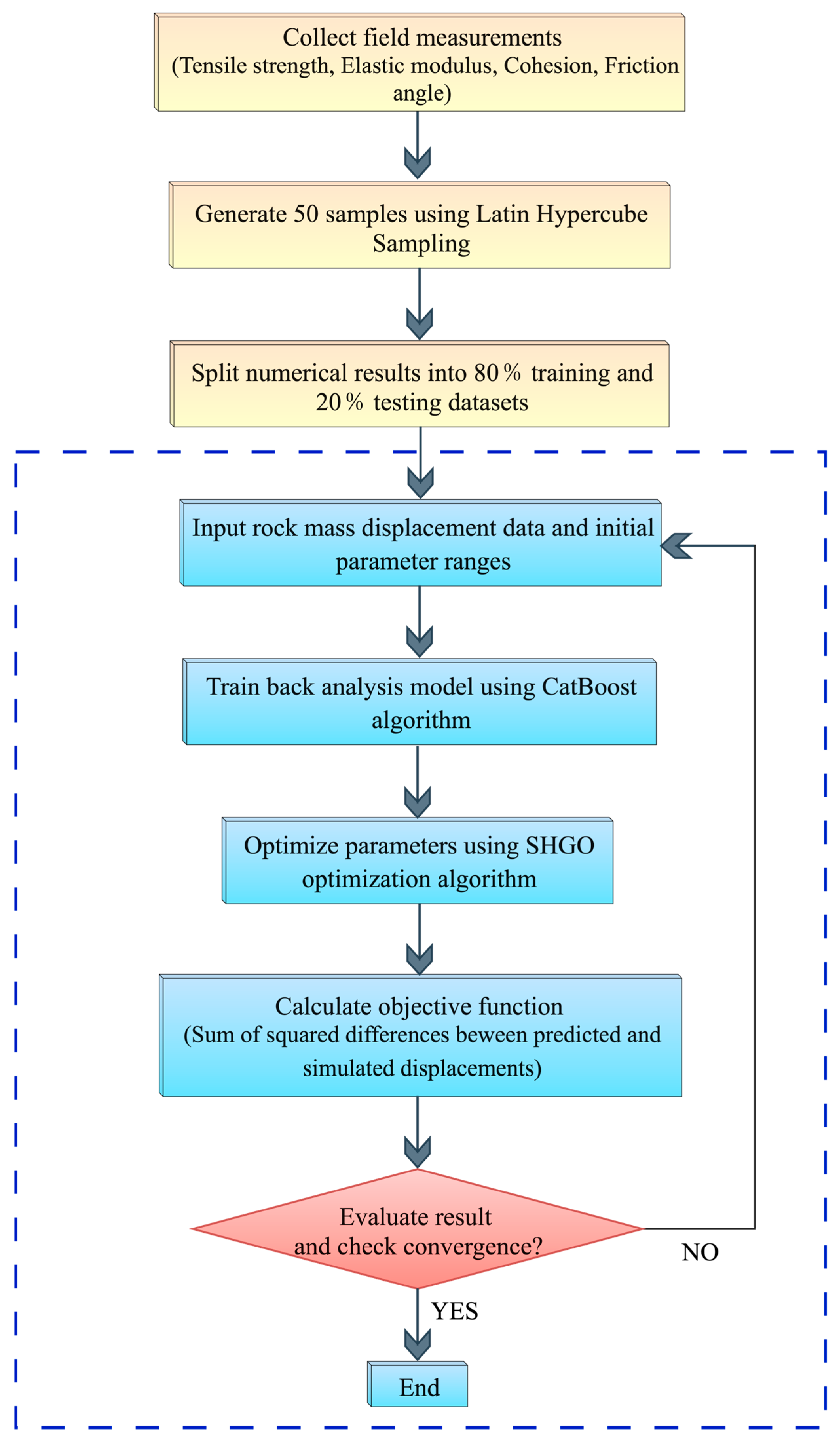
A novel inverse-analysis framework is proposed, integrating the CatBoost algorithm for surrogate model development and the SHGO algorithm. The surrogate model, which describes the relationship between the rock mass properties and their responses during excavation, is established using CatBoost. In the inverse analysis process, SHGO algorithm is employed to identify the optimal parameters. The flowchart of the proposed framework is presented in Figure 2. The detailed procedure is as follows:
Step 1: Collect the in situ measured mechanical parameters of the rock mass, including tensile strength, elastic modulus, cohesion, and internal friction angle, for parameter inversion.
Step 2: Generate 50 samples using the Latin hypercube sampling method. Allocate 80% of these as training samples and 20% as validation samples. Fifty sets of rock mass parameter combinations should be created within the initial parameter range, which is detailed in Table S1 (refer to Supplementary Materials).
Step 3: Conduct numerical simulations in FLAC3D to calculate the displacement changes at the monitoring points.
Step 4: Train the inverse analysis model using the CatBoost algorithm. The model’s inputs will consist of the four rock mass parameter characteristics, while the outputs will be the displacements of 20 monitoring points over 28 steps. Set the training parameters as follows: iterations = 1000, depth = 6, learning rate = 0.05, and L2 regularization = 3.
Step 5: Perform parameter optimization using the SHGO algorithm.
Step 6: Input the surrounding rock displacement data obtained from the numerical simulations, along with the initial range of rock mass parameters.
Step 7: Conduct inversion calculations using the data-driven algorithm.
Step 8: Evaluate the results and check whether the convergence criteria are met.
Step 9: If the convergence criteria are not met, repeat from Step 6 until the termination conditions are satisfied to find the optimal solution.

4. Application

To verify the performance of the developed displacement-based inversion analysis model, it was applied to the excavation process of the D2 laboratory in Phase II of the Jinping Underground Laboratory in China for the inversion analysis of the surrounding rock mass parameters. The reliability of the developed model was demonstrated, and the inversion results of the surrounding rock parameters under different conditions were further discussed, which further confirmed the generalization and robustness of the framework developed in this study.

4.1. Numerical Model of Tunnel in Jinping Underground Laboratory

To conduct inversion analysis, this study proposes a model based on FLAC3D numerical simulation. The core of the numerical model is the strain-softening model implemented within the finite-difference framework of FLAC3D, and a three-node triangular element mesh is employed. The model comprises 455,888 triangular elements and 227,945 nodes, offering a detailed discretization of the rock mass (see Figure 3a). In terms of the rock mass constitutive model, the strain-softening model is adopted. This model can better capture the nonlinear deformation and failure characteristics of the rock mass during the excavation process. For the strength criterion, the Mohr–Coulomb criterion is used to describe the rock mass. To verify the performance of the proposed displacement-based inversion analysis model, the model was applied to the excavation of the D2 laboratory, a component of the second-phase project of the Jinping Underground Laboratory (CJPL–II) in China. The exposed chamber of the D2 laboratory after completion of excavation is shown in Figure 3c.
Although Jinping marble is classified as a hard rock and exhibits local joints, field investigations and previous studies [41,42,43] have shown that the instability mode of the surrounding rock at the Jinping Laboratory is mainly stress-induced splitting and spalling, rather than block sliding along continuous joints. The average joint spacing exceeds 1 m. It is tightly closed by high confining pressure (burial depth of 2400 m), with negligible contributions of joint opening and slip to the overall displacement. Therefore, the FLAC3D strain-softening continuum model is sufficient to capture the main mechanical behavior. Moreover, the core objective of this study is to obtain equivalent rock mass parameters through displacement inversion, rather than precisely tracking local deformation of structural surfaces. Thus, the strategy of using FLAC3D for modeling achieves a reasonable balance between accuracy and engineering practicality.
Four boreholes were drilled from the service tunnel D to the D2 laboratory, numbered No. 1, No. 2, No. 3, and No. 4, respectively. Each borehole has a depth of 8.5 m and heights of 2 m, 4 m, 10 m, and 14 m, respectively (see Figure 3b). Multi-point displacement meters were pre-installed in these boreholes, with five monitoring points set up in each borehole, located at distances of 0.5 m, 2.5 m, 4.5 m, 6.5 m, and 8.5 m from the tunnel wall, denoted as d1, d2, d3, d4, and d5, respectively. Throughout the construction period, the deformation of the surrounding rock at different depths in each borehole was monitored through these sensors. The entire excavation process was divided into 28 distinct steps, and the displacement changes in the surrounding rock were continuously monitored in situ during the construction process. The displacement data of the multi-point displacement meter in borehole No.1 are shown in Table 1. The initial true values of four key surrounding rock parameters ( σ t , E , c , and φ ) were obtained from the field tests and are listed in Table 2. To facilitate inverse analysis, the Latin hypercube sampling method was employed to generate 50 sets of samples for the surrounding rock parameters. These samples were then divided into a training dataset (80%) and a testing dataset (20%). The samples were input into the numerical simulation software to calculate the displacement data of the 20 monitoring points in the four boreholes across the 28 excavation steps.

4.2. Results

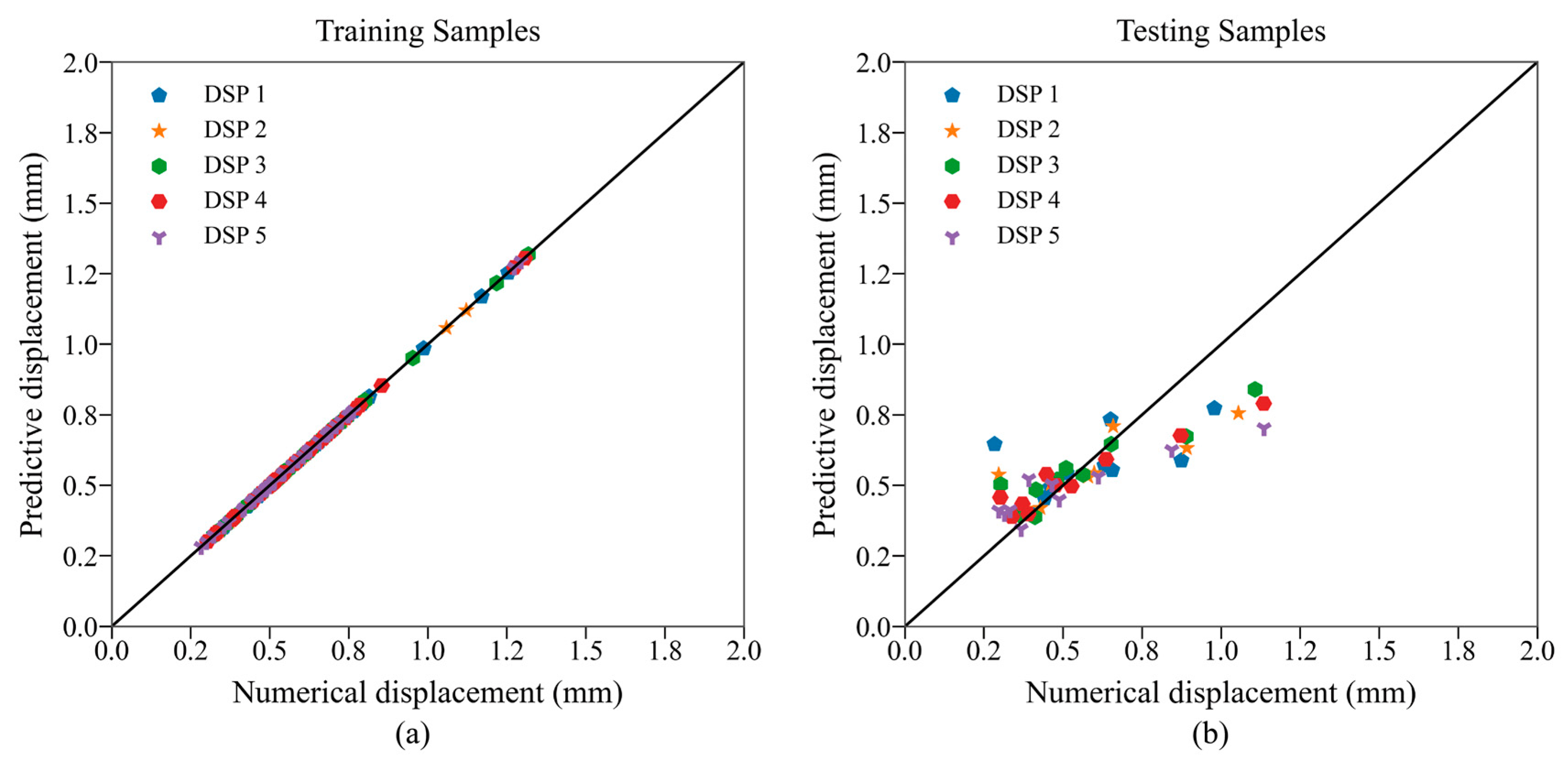
To verify the feasibility of the inverse analysis method, the displacement data of five points were first input into the inverse analysis model. The results of the training samples and monitoring samples are presented in Figure 4. The displacements of most test samples align well with the numerical model results, and the differences between most test and training samples are less than 0.3 mm, with a maximum relative error of 8.7%. This indicates that the established surrogate model accurately reflects the nonlinear behavior of the surrounding rock, and the performance is satisfactory. Under the balance of efficiency and performance, the surrogate model is considered a good choice for inverse analysis.
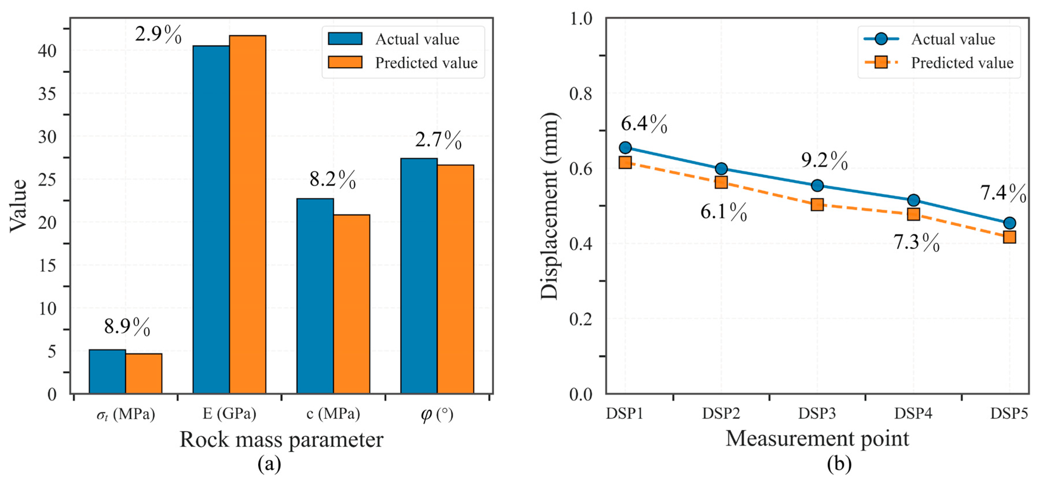
To obtain appropriate surrounding rock parameters through inverse analysis, an optimization process based on SHGO was carried out within the proposed framework using numerical simulation results and the derived inverse analysis surrogate model. The displacements obtained from numerical simulation and surrounding rock parameters within a given range were input, and the optimized surrounding rock parameters are shown in Table 3. The relative errors of the optimized surrounding rock parameters and the relative errors between the predicted displacements and the numerically simulated displacements are shown in Figure 5. The errors are negligible, with the maximum displacement error being 9.2% and the maximum parameter error being 8.9%. The results demonstrate that the developed framework accurately characterizes the rock mass’s mechanical behavior.
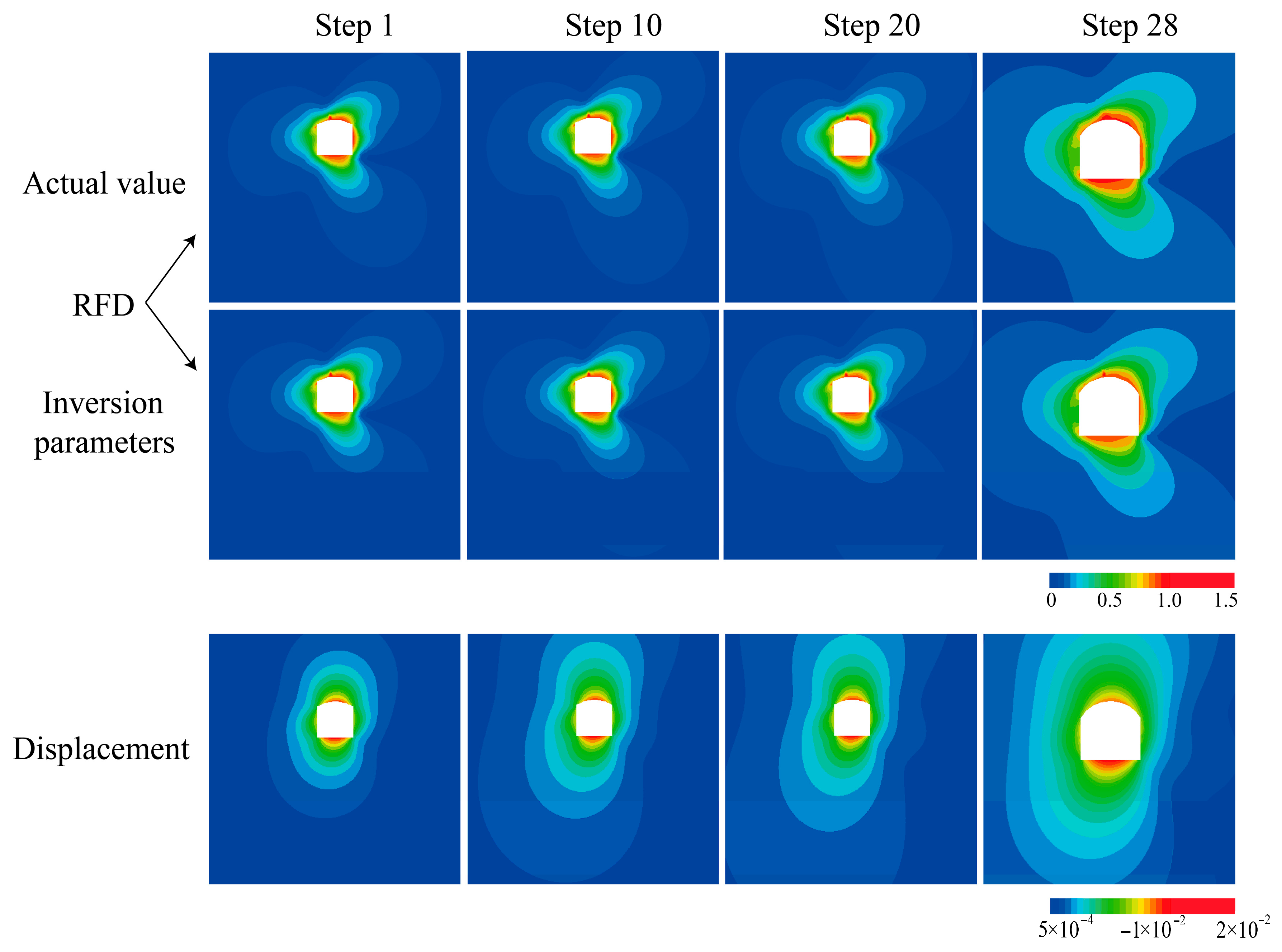
In order to further investigate the developed framework, the obtained rock mechanical parameters were used to compute the degree of surrounding rock failure (RFD). The expression of RFD is seen in Equations (15) and (16):
R F D = q g ( θ ) A p 2 + B p + C ( b e f o r e   t h e   p e a k   s t r e n g t h ) 1 + ε s / t p / ε s / t p l i m ( a f t e r   t h e   p e a k   s t r e n g t h )
p = ( σ 1 + σ 2 + σ 3 ) q = ( σ 1 2 σ 2 2 + σ 2 2 σ 3 2 + σ 3 2 σ 1 2 / 2
where σ 1 , σ 2 , and σ 3 present the maximum, intermediate, and minimum principal stresses, respectively. g θ is the plastic potential function. A , B , and C are all strength criterion variables. p represents the mean principal stress, and q represents generalized shear stress. ε s / t p represents the current plastic shear/tensile strain, and ε s / t p l i m represents the ultimate plastic shear/tensile strain. When R F D 1.0 , the rock mass within this range begins to break [42,43].
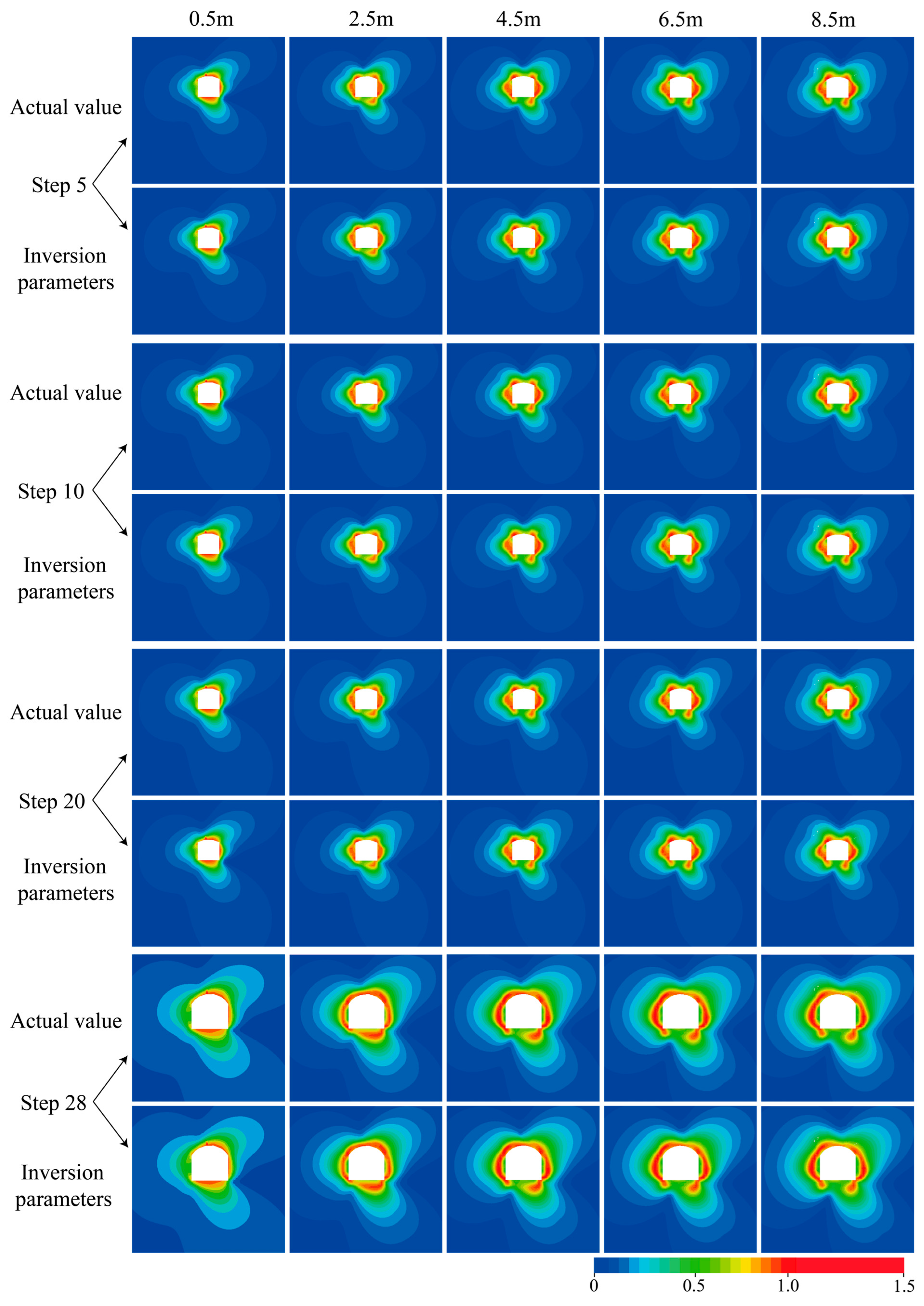
By inputting the inverted surrounding rock parameters into the numerical model, a comparison chart of RFD and the true value can be obtained. The difference between the two is very small. In addition, a contour map of the surrounding rock displacement under the characteristic excavation steps can also be obtained (see Figure 6). The above analysis further confirms the reliability of the inverse analysis model proposed in this study. It further demonstrated that the rock mechanical parameters obtained using the developed framework accurately characterize the deformation and failure mechanisms of the surrounding rock mass.

4.3. Discussions

4.3.1. Temporal Evolution of Inversion Accuracy

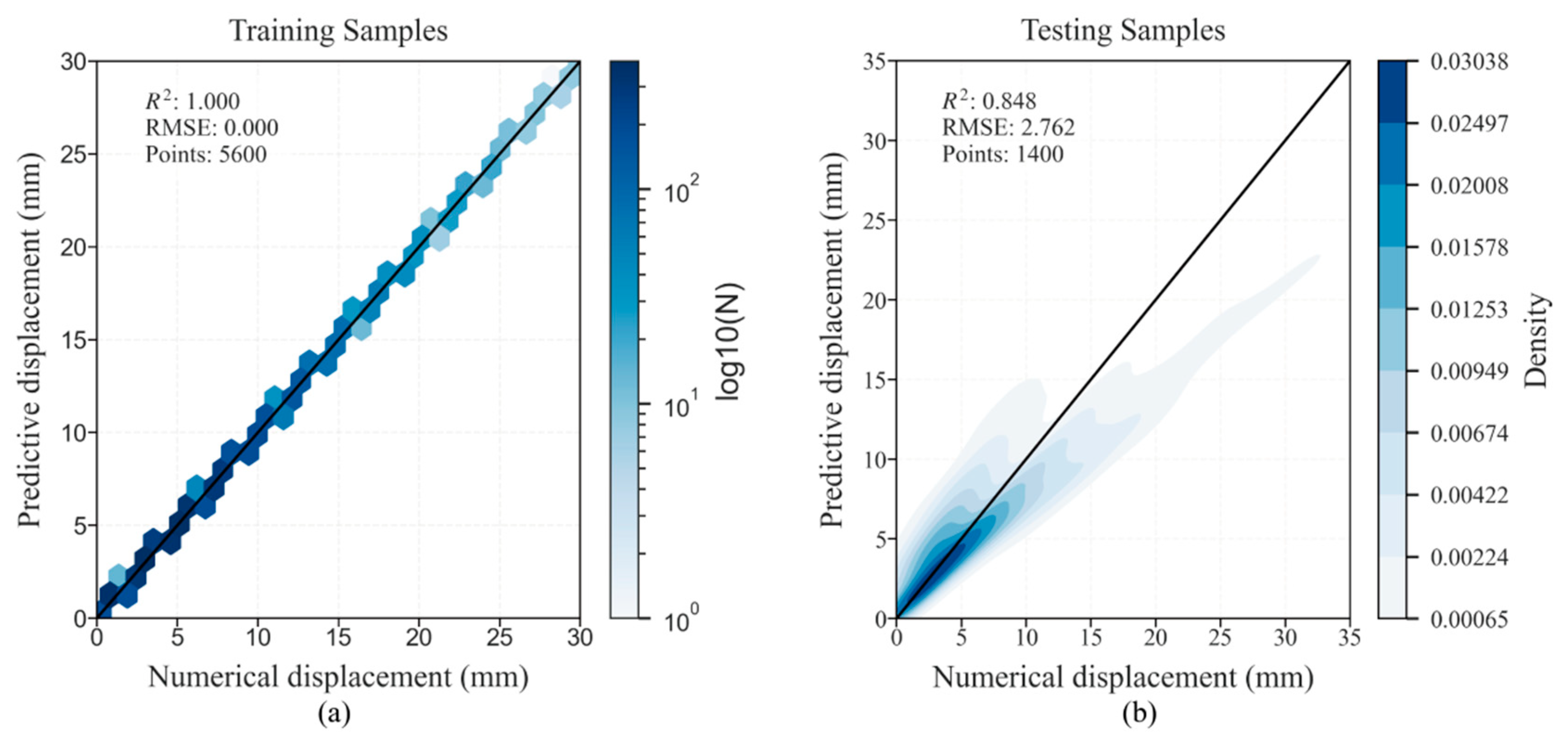
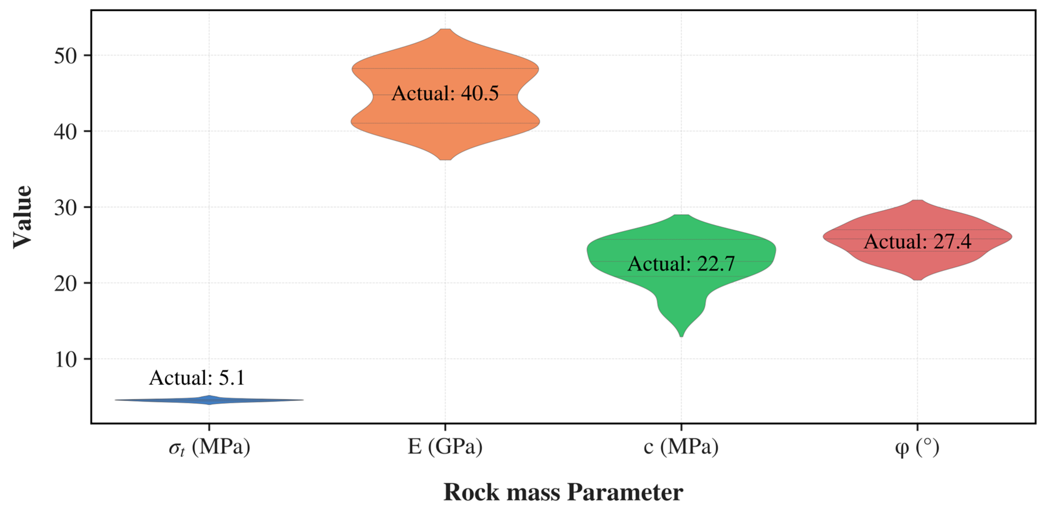
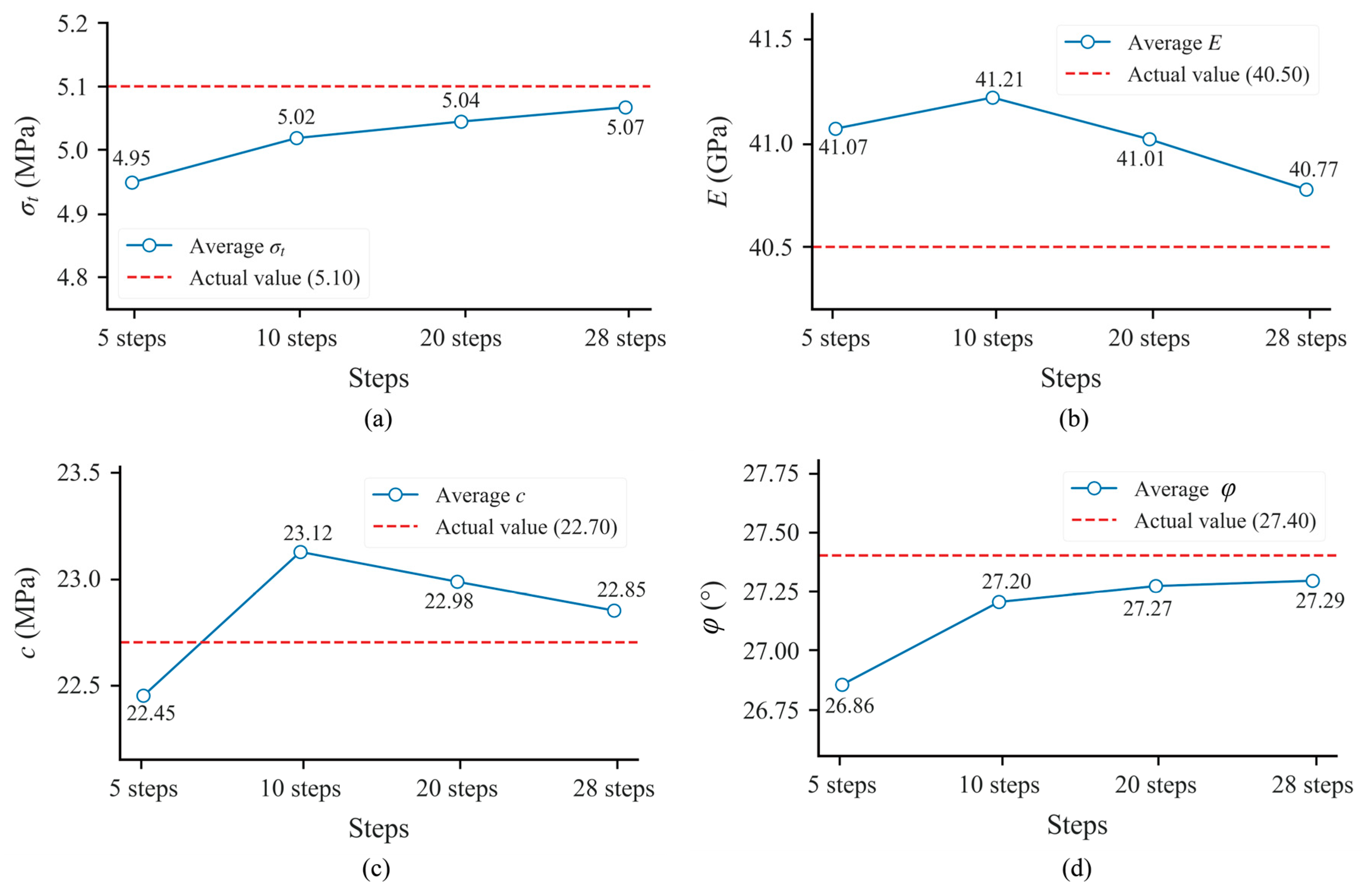
Based on the validation results of the inverse analysis model described above, the performance of the surrogate model has been verified. To further illustrate the generalization capability of the surrogate model, displacement values from the 28 excavation steps of hole 1 were used, with 80% allocated for training and 20% for validation, as shown in Figure 7. The validation sample achieved a fit of 84.8%, indicating excellent performance of the inverse analysis model. Similarly, given a set of accurate numerical simulation displacements and a range of surrounding rock parameters, these parameters can be optimized for each excavation step. The predicted trend of the 28 sets of surrounding rock parameters is shown in Figure 8, with the average values of the parameters being close to the true initial values. To more intuitively demonstrate the inversion effect of the surrogate model at each excavation step, comparisons were made between the first 5 steps and the first 10 steps, the first 10 steps and the first 15 steps, the first 15 steps and the first 20 steps, and the first 20 steps and the complete excavation steps. The average values of the inverted parameters were compared with the true values, and the relative errors were calculated, as shown in Figure 9. The relative errors were all within 5%, proving the generalization capability of the surrogate model. Based on a comprehensive analysis, it is concluded that utilizing full-stage displacement data in the actual inverse analysis process yields the most accurate parameters for dynamic construction control.

4.3.2. Spatial Robustness with Multiple Boreholes

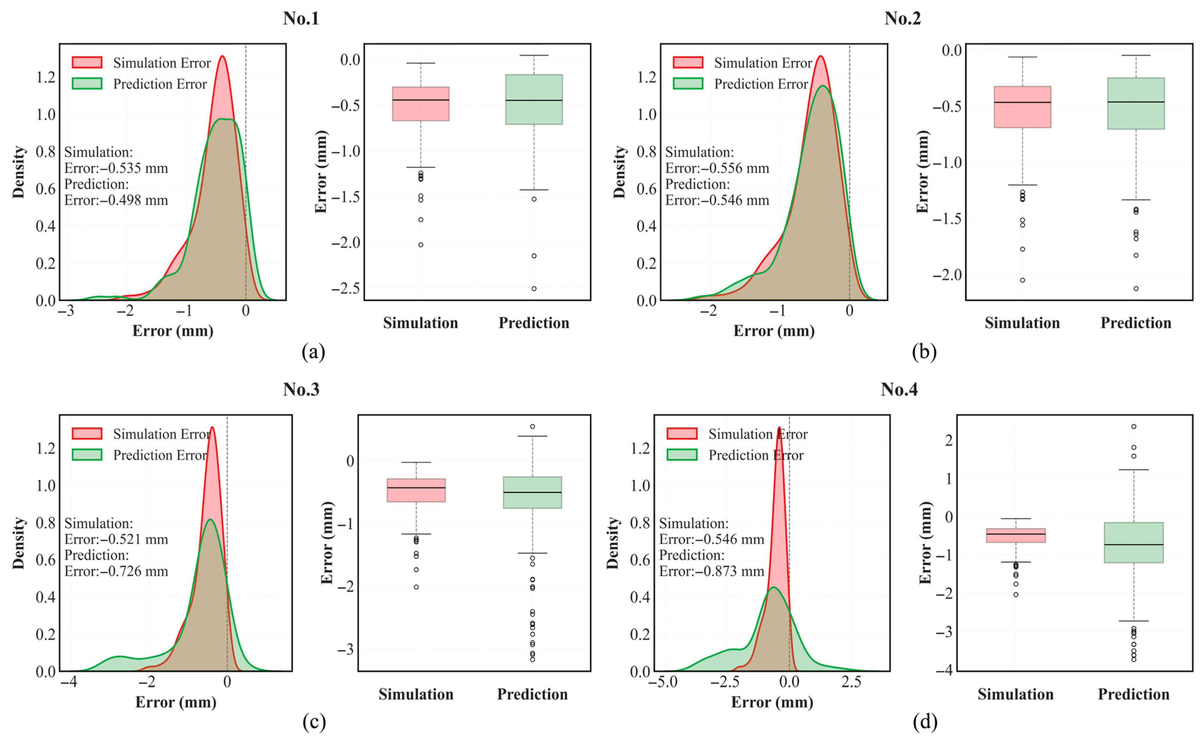
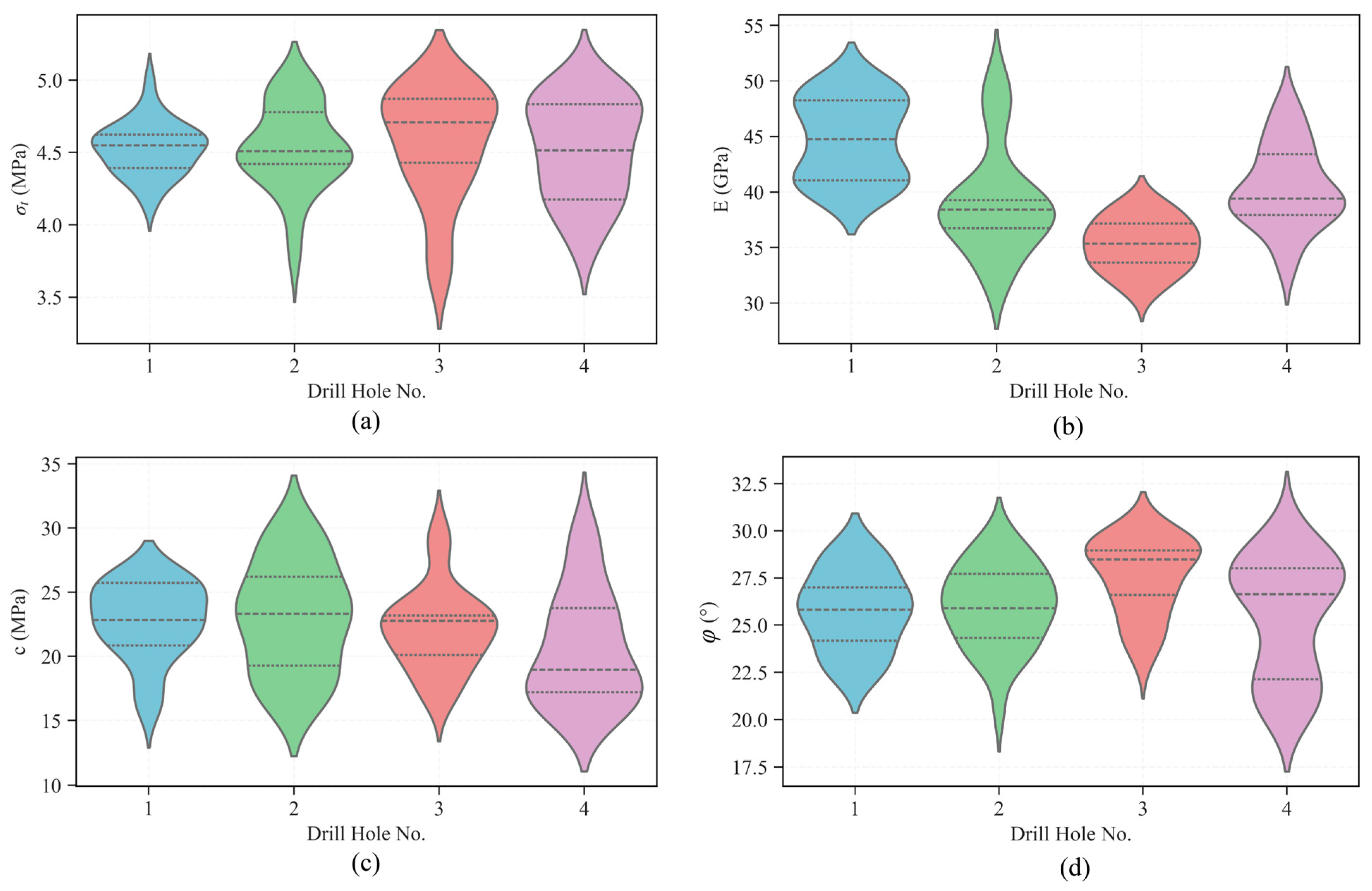
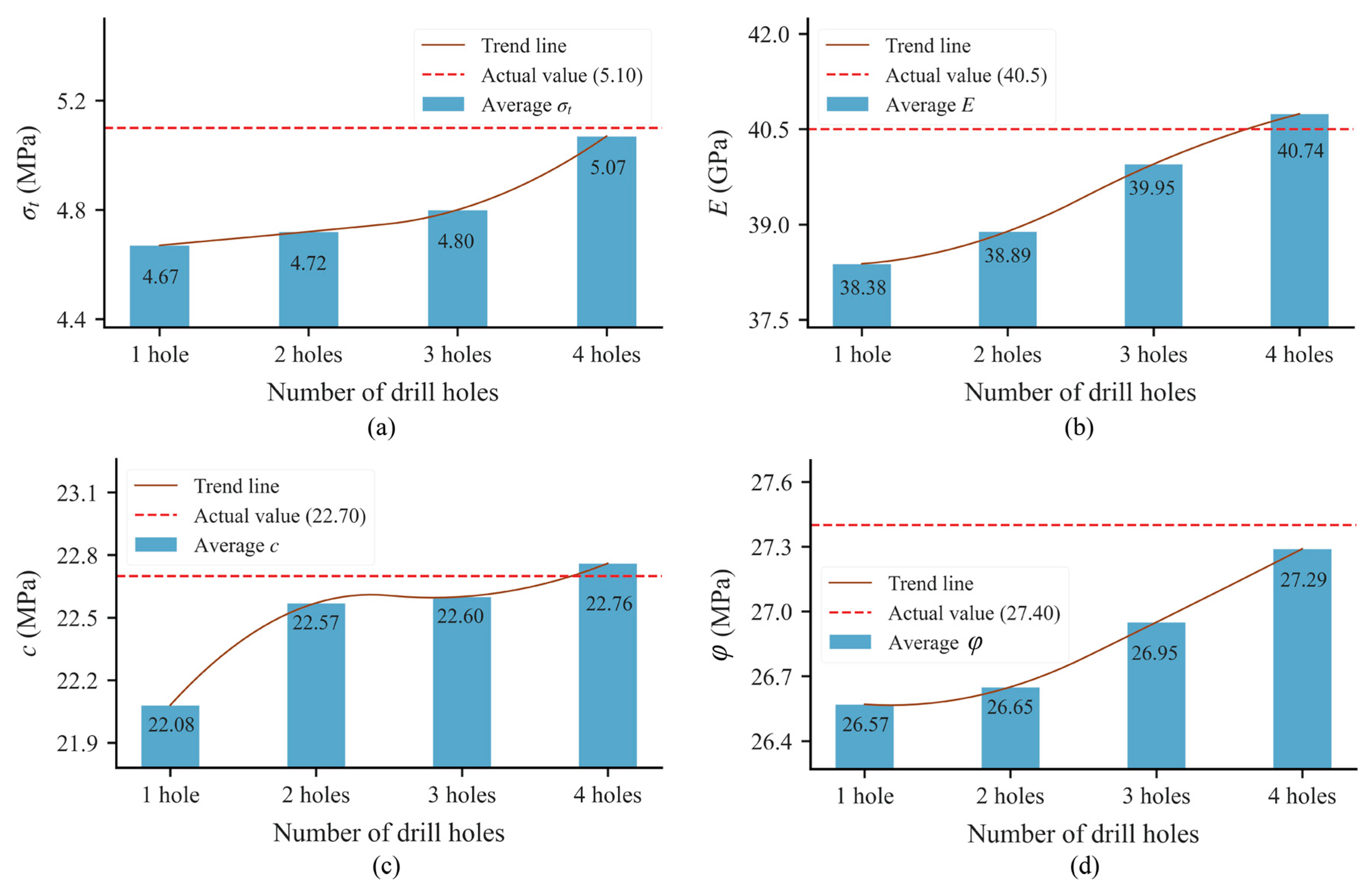
The validation described above demonstrated that the difference in surrounding rock parameters inverted using the surrogate model at different excavation steps within the same borehole is very small, indicating the model’s generalization capability. To obtain a more comprehensive evaluation of the parameter inversion effects, the displacements from all four monitoring boreholes were incorporated into the inverse analysis. The average of the inversion displacements of the four boreholes was compared with accurate and field measurements (see Figure 10). The maximum error was found to be only 0.8733 mm, demonstrating the accuracy of the proxy model in predicting displacement during the reverse analysis. In addition, the surrounding rock parameters are optimized through inversion. For the four surrounding rock parameters, the average values of three parameters are consistent across the four boreholes, except for the elastic modulus ( E ). The mean of E varies more significantly among the four boreholes. However, the maximum error in E between boreholes one and three is still controlled within 20% (see Figure 11). Figure 12 shows the changes in the average values of the inverted parameters as the number of boreholes increases. Based on the analysis, multi-source monitoring significantly enhances the overall reliability of parameter inversion.

4.3.3. Robustness Against Parameter Range Uncertainty

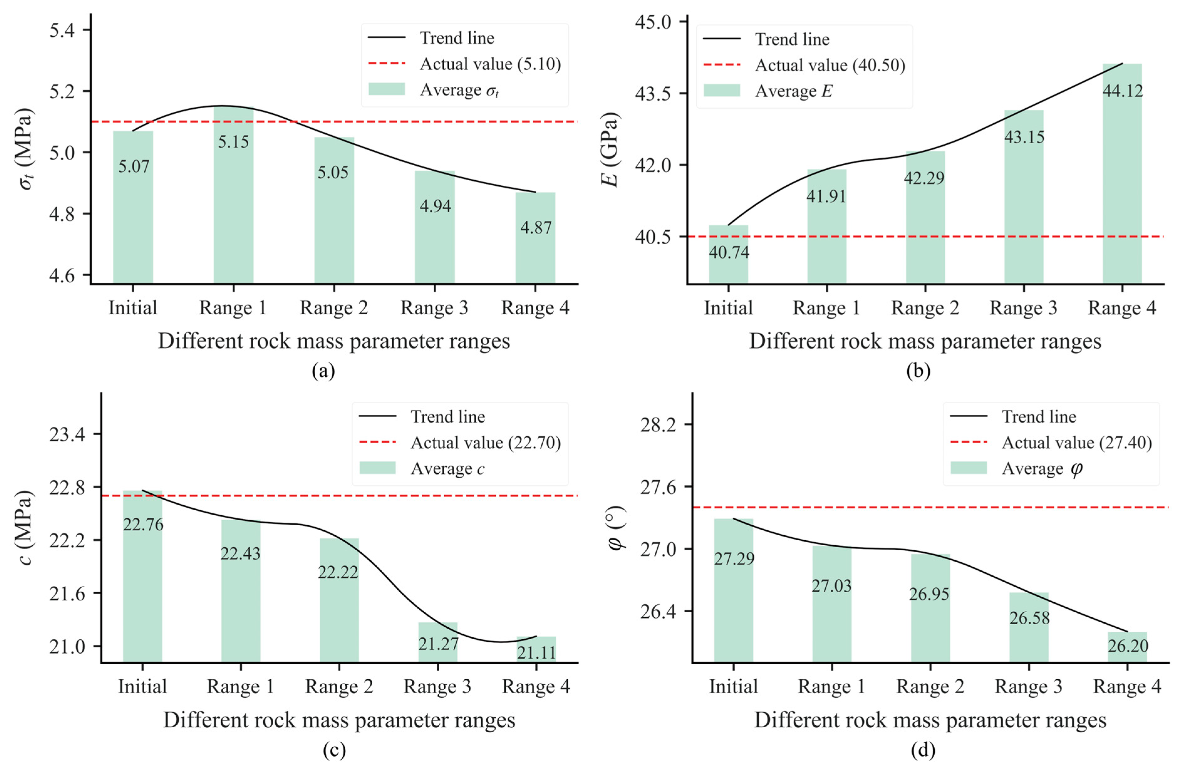
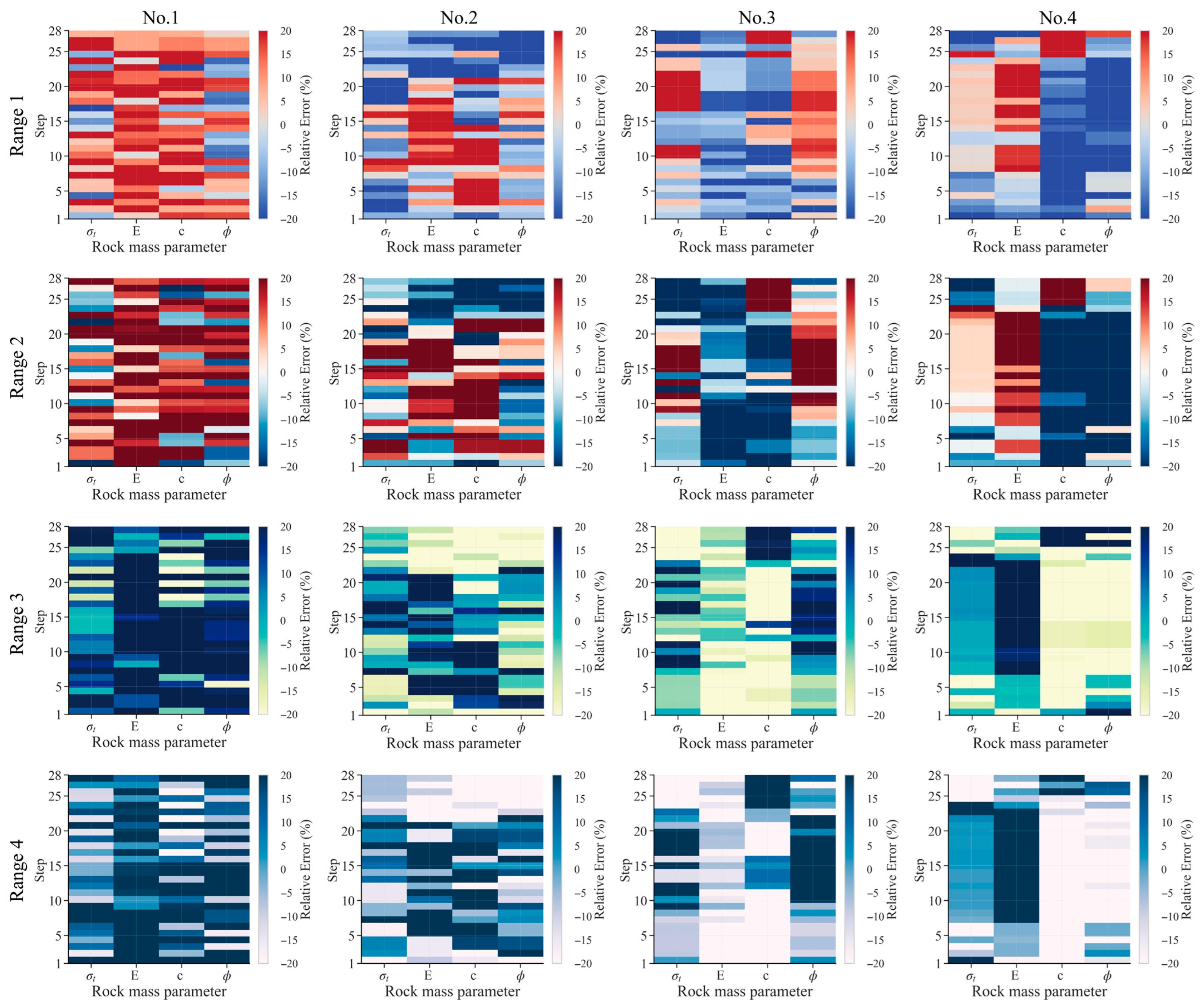
While the discussions above on different excavation steps and monitoring from various boreholes have validated the surrogate model in the inverse analysis process, they have overlooked the fact that the input displacement is a fixed value, whereas the parameters are within a range. It is not clear whether the selection of optimal parameters would change with variations in the size of the parameter range. In this study, the initial ranges for the four parameters and the values for incrementally expanding these ranges are presented in Table 4. The four rock mass parameter ranges are applied to the four boreholes for calculation. The average values of the four inverted parameters within each range are compared with the true values, including the initial parameter ranges (see Figure 13). To provide a more intuitive comparison, the data for each borehole within each parameter range are displayed separately and compared with the true values. For example, Range1-No.1 indicates the relative error between the inverted values and the true values of the four parameters in the first borehole under the first parameter range. The depth of the heatmap color represents the magnitude of the relative error. This is repeated for the four different parameter ranges corresponding to the four boreholes, resulting in 16 heatmap comparison figures (see Figure 14). Based on the analysis, the model tolerates significant initial parameter uncertainty, which is critical for field applications with limited prior knowledge. As the range of surrounding rock parameters continues to expand, the average values of the inverted parameters increasingly deviate from the true values. However, the maximum error remains within 20%, which further confirms the good performance of the inversion model and the accuracy of the inverse analysis.

4.3.4. Validation via Mechanical Response Prediction

The preceding three sections have discussed the impact of different excavation steps, various boreholes, and the range of surrounding rock parameters on inverse analysis. Given the comprehensive analysis conducted, the optimal surrounding rock parameters obtained from each range were averaged. These average parameter values were then input into the numerical simulation software. The average values of the parameters are as follows: tensile strength ( σ t ) is 4.965, Young’s modulus ( E ) is 42.278, cohesion ( c ) is 21.389, and the internal friction angle ( φ ) is 26.649. The inverted parameters were analyzed in terms of the mechanical properties of the surrounding rock in the excavated chamber (RFD). Comparisons were made at various excavation stages between the results simulated using the actual initial surrounding rock parameters and those using the inverted parameters. To vividly demonstrate the accuracy of the optimal inverted parameters obtained through inverse analysis, comparisons of the RFD contour maps at the 5th, 10th, 20th, and 28th excavation steps were made for the five monitoring locations (0.5 m, 2.5 m, 4.5 m, 6.5 m, and 8.5 m) of the multi-point displacement meters in the four boreholes (see Figure 15). Based on the analysis, the relative error between the RFD cloud diagrams obtained from the inverted parameters and the actual parameters is less than 5%, thereby confirming that the inverted parameters can accurately predict rock mass behavior and enable reliable early-stage support design.

4.3.5. Parameter Interdependence and Sensitivity-Driven Optimization

The Pearson correlation coefficient, ranging from −1 to 1, measures the linear relationship between two variables, with values closer to 1 or −1 indicating a stronger correlation. In this study, 50 samples generated using Latin hypercube sampling were analyzed for correlation among four surrounding rock parameters: elastic modulus, tensile strength, cohesion, and internal friction angle (see Figure 16). The correlation coefficients are 0.38, −0.16, −0.09, −0.09, −0.30, and 0.11, showing varying linear relationships. The strongest correlation is between elastic modulus and tensile strength (0.38). During inverse analysis of rock response (displacement), multiple combinations of these parameters may fit the monitored data, potentially affecting the accuracy of the inversion results.
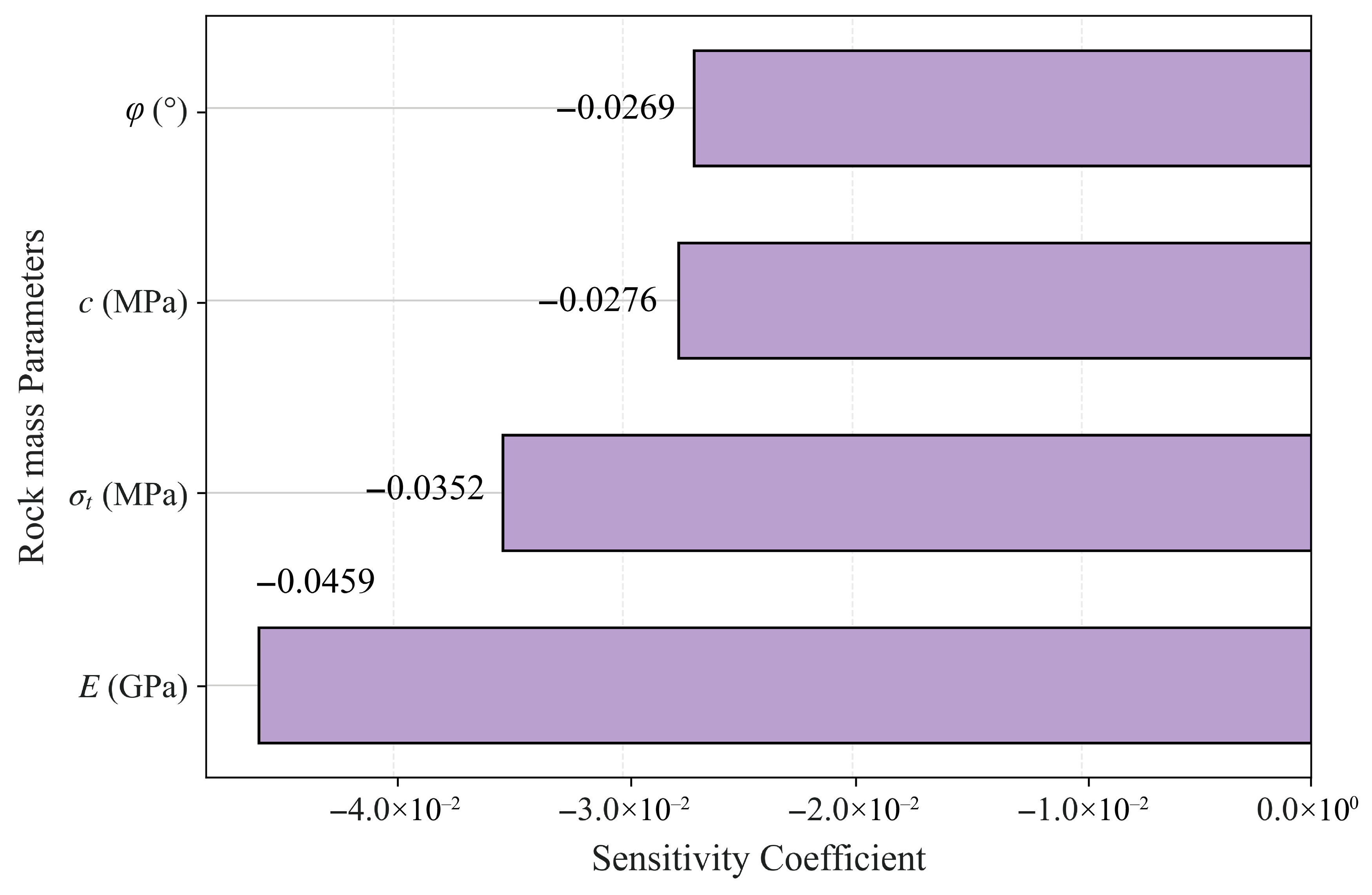
Subsequently, a sensitivity analysis was conducted to determine the degree of sensitivity of each parameter to the surrounding rock response (displacement). Parameters with higher sensitivity have a greater impact on the surrounding rock response. As shown in Figure 17, the parameter c (cohesion) has the lowest correlation with the other three parameters, followed by φ , σ t , and E . To quantify this, the cohesion c was increased by 10%, while keeping the other parameters constant, and the model was recalculated to observe the change in displacement at a specific point. The ratio of the displacement changes to the change in the parameter c was used as the sensitivity coefficient. This process was repeated by incrementally increasing the other three parameters by 10%, one at a time, and recalculating the displacements. The sensitivity coefficients were then determined by comparing the recalculated displacements to the initial numerical simulation results at randomly selected monitoring points.
The elastic modulus directly controls the initial deformation of the rock mass under stress, which makes it the parameter with the most significant fluctuation among all parameters. Since the monitored displacements are primarily within the elastic or early plastic deformation stage, variations in the elastic modulus produce the most significant changes in displacement. In contrast, other parameters, such as cohesion or friction angle, mainly affect the failure threshold or post-yield behavior. Therefore, the sensitivity coefficient of the elastic modulus is naturally higher.
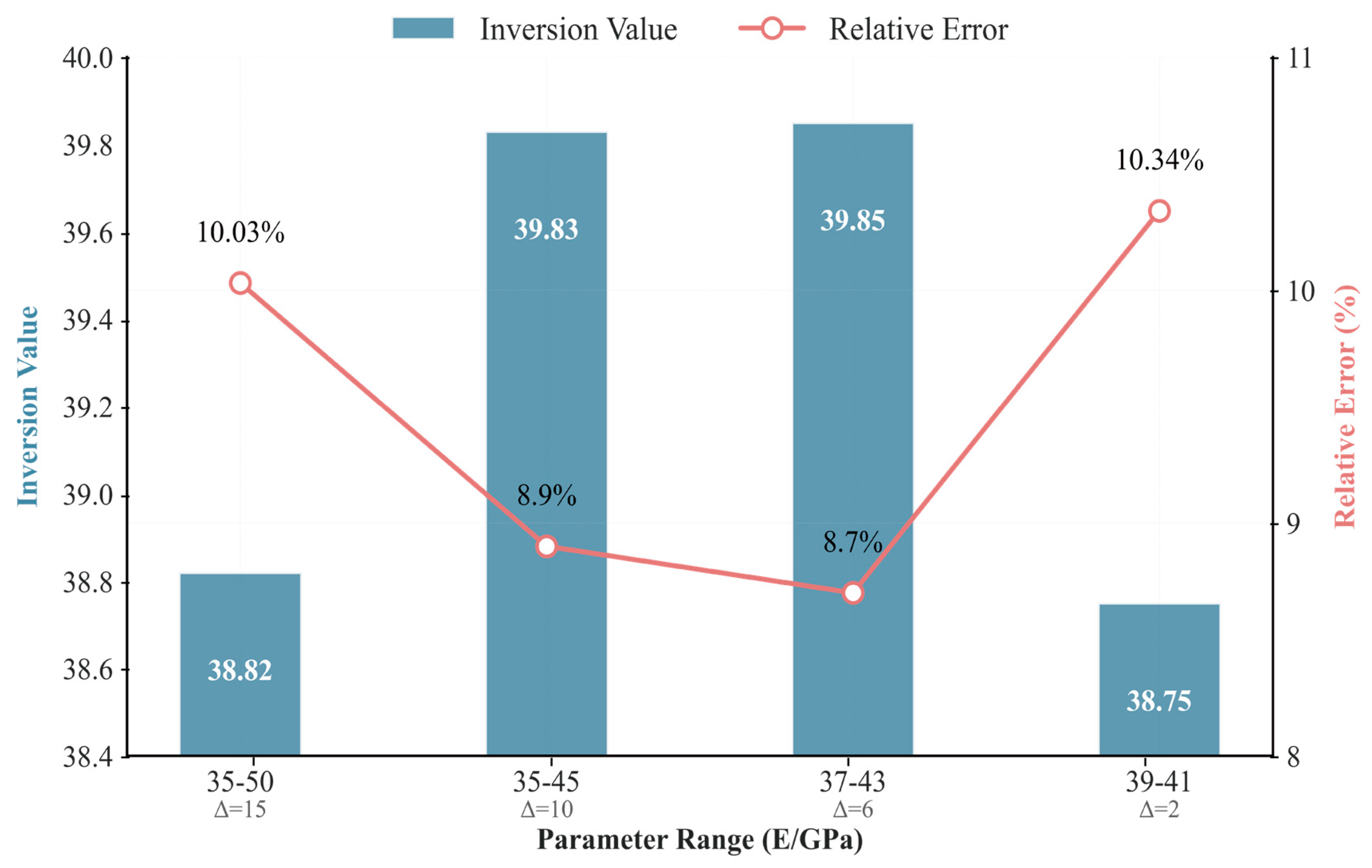
Based on the calculations described above, the sensitivity coefficient for the elastic modulus E was found to be the highest. A similar objective function, as established in Section 3.4, was developed to quantify the discrepancy between the simulated displacements and the actual monitored displacements. By iteratively varying the range of E while keeping the other three parameters constant, and incorporating these into the inverse analysis model, an optimization algorithm was employed to iteratively identify the optimal value of E that minimizes the objective function. Each candidate value of E was subsequently input into the numerical simulation to compute the corresponding displacements and update the objective function value, continuing this process until the value of E that minimizes the objective function was identified. As illustrated in the figure, the comprehensive results of multiple optimizations revealed that when E = 39.85, the relative error was minimized (11%). Therefore, E = 39.85 was ultimately determined to be the optimal parameter value (see Figure 18). Based on the analysis, it has demonstrated superior performance in terms of accuracy and reliability, and can serve as a robust foundation for subsequent engineering analysis and design.

4.4. Validation of D2 Laboratory Operation Data

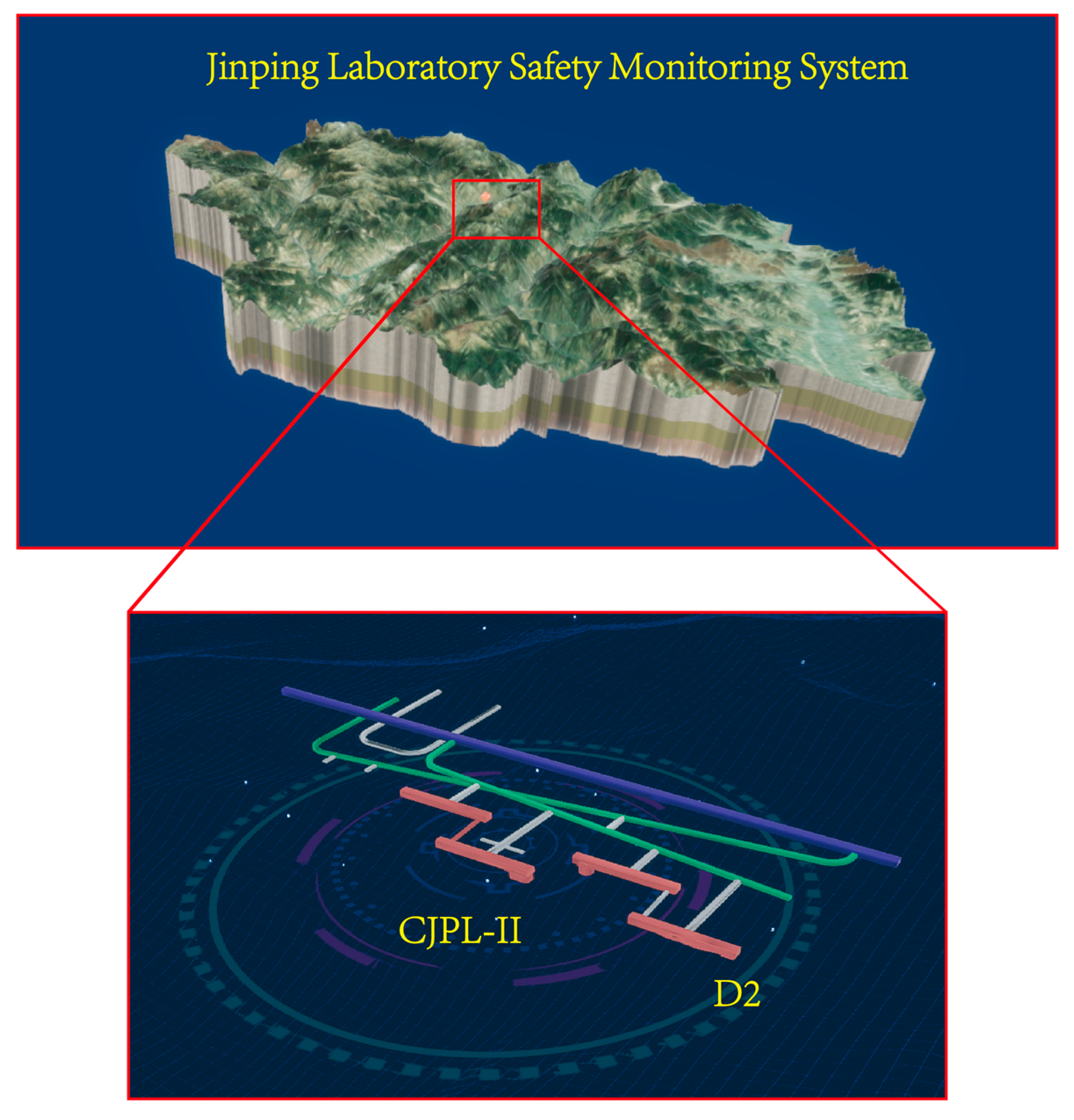
This study utilized D2 laboratory displacement sensor DSP(a) data, obtained from the CJPL-II experimental hall during 2021–2025, as part of the Jinping Laboratory safety monitoring system (see Supplementary Materials, Table S2) [44]. The system features a 3D visualization platform based on a BIM model, enabling real-time visualization of rock mass and facility conditions, and providing intuitive support for geological and structural safety management. (see Figure 19). To invert the rock mass parameters, displacement data from 1 September to 30 September 2022 (30 days in total) were used as the training set, and the CatBoost–SHGO method was applied to obtain a real-time sequence of rock mass parameters. Subsequently, displacement data from 1 December to 30 December 2024, were used for blind validation (Table S2 contains 60 rows, with the first 30 rows used for training and the remaining 30 for validation).
The inversion results show that the average elastic modulus E during the training period was 39.69 GPa, differing by only 2.0% from the reference value of 40.5 GPa obtained during construction. In the blind validation phase, the displacement prediction achieved a coefficient of determination R 2 = 0.954 with a maximum residual of 0.002516 mm (see Figure 20). Moreover, following the seismic event on 30 July 2025, the monitoring system recorded a sudden displacement increase by 0.08 mm, and the inversion results indicated a decrease in approximately 7.5% in the frictional cohesion c suggesting a significant impact of the earthquake on rock mass mechanical properties. This event also caused localized bare rock spalling along the laboratory sidewall and detachment of the lining beneath the ventilation ducts (see Figure 21). The laboratory operation team promptly reinforced the affected areas with steel arches and lining supports, effectively mitigating potential safety risks.

5. Conclusions

Inverse analysis serves as a critical methodology for determining the mechanical properties of rock masses in deep underground engineering. This study presents an innovative framework that integrates the data-driven CatBoost algorithm with the SHGO method. The framework utilizes CatBoost to efficiently construct a high-fidelity surrogate model that captures the relationship between surrounding rock displacement and mechanical parameters. At the same time, SHGO (a derivative-free optimization algorithm requiring only objective function evaluations) performs parameter inversion. This integration significantly enhances the computational robustness and reliability of the inverse analysis process. To validate the framework, we applied it to the D2 laboratory of the second phase project of the Jinping Underground Laboratory (CJPL–II) in the China case study. Based on in situ displacement monitoring data and FLAC3D numerical simulations, we established a high-accuracy surrogate model. Systematic investigation of inversion results across varying excavation steps, borehole monitoring configurations, and expanded rock mass parameter ranges revealed the following key patterns:
  • Validation of the established surrogate model, combined with the SHGO process, yielded optimized surrounding rock parameters with minimal relative errors, confirming satisfactory inverse analysis results. Furthermore, substituting these inverted parameters into the numerical model produced mechanical responses of the surrounding rock that closely matched the true values, demonstrating the model’s reliability.
  • In practical inverse analysis, using displacement data from the first 28 steps yields rock parameters closer to the true values. Furthermore, increasing the number of measurement holes further enhances the accuracy of the inverted parameter averages.
  • As the range of surrounding rock parameters widens, the deviation of the inverted parameter averages from their true values increases. Nevertheless, the maximum error consistently remains below 20%, demonstrating the model’s robust inversion performance and high accuracy.
  • In the inverse analysis results, the relative error between RFD cloud diagrams generated using the inverted parameters and those based on the actual parameters is below 5%. Sensitivity analysis revealed the elastic modulus E as the most influential parameter.
  • The optimization algorithm determined the optimal E value to be 39.85, achieving the minimum relative error. These results provide a robust basis for subsequent engineering analysis and design.

Supplementary Materials

The following supporting information can be downloaded at: https://www.mdpi.com/article/10.3390/buildings15173187/s1, Table S1: LHS Samples; Table S2: Table of long-term displacement monitoring.

Author Contributions

Methodology, H.Z.; software, M.S.; validation, J.Y.; formal analysis, M.S., Y.X. and S.L.; investigation, M.Z.; data curation, Z.F. and J.Y.; writing—original draft preparation, Z.F.; writing—review and editing, S.L.; visualization, P.P.; supervision, M.Z.; funding acquisition, H.Z., Y.X. and P.P. All authors have read and agreed to the published version of the manuscript.

Funding

This research was funded by the National Natural Science Foundation of China (grant nos. 52125903, 42377174, and 42172317) and the Natural Science Foundation of Shandong Province, China (grant no. ZR2022ME198). And The APC was funded by the National Natural Science Foundation of China (grant no. 42172317).

Acknowledgments

The authors gratefully acknowledge the support received for this work.

Conflicts of Interest

Authors Manbin Shen and Jinzhong Yang are employed by the Yalong River Hydropower Development Co., Ltd. The remaining authors declare that the research was conducted in the absence of any commercial or financial relationships that could be construed as a potential conflict of interest.

References

  1. Li, C.; Wang, L.; Li, J.; Chen, Y. Application of multi-algorithm ensemble methods in high-dimensional and small-sample data of geotechnical engineering: A case study of swelling pressure of expansive soils. J. Rock Mech. Geotech. Eng. 2024, 16, 1896–1917. [Google Scholar] [CrossRef]
  2. Ullah, J.; Huan, L.; Zuo, Y.H.; Ehsan, M.; Soupios, P. Enhancing Reservoir Characterization: Genetic Algorithm-Assisted Correction of Pore Aspect Ratio Using CNN-LSTM in Petrophysical Modeling. IEEE Trans. Geosci. Remote Sens. 2025, 63, 5908311. [Google Scholar] [CrossRef]
  3. Pinheiro, M.; Vallejos, J.; Miranda, T.; Emery, X. Geostatistical simulation to map the spatial heterogeneity of geomechanical parameters: A case study with rock mass rating. Eng. Geol. 2016, 205, 93–103. [Google Scholar] [CrossRef]
  4. Hu, X.; Shentu, J.; Xie, N.; Huang, Y.; Lei, G.; Hu, H.; Guo, P.; Gong, X. Predicting triaxial compressive strength of high-temperature treated rock using machine learning techniques. J. Rock Mech. Geotech. Eng. 2023, 15, 2072–2082. [Google Scholar] [CrossRef]
  5. Zhao, H.; Li, S.; Zang, X.; Liu, X.; Zhang, L.; Ren, J. Uncertainty quantification of inverse analysis for geomaterials using probabilistic programming. J. Rock Mech. Geotech. Eng. 2024, 16, 895–908. [Google Scholar] [CrossRef]
  6. Sakurai, S.; Takeuchi, K. Back analysis of measured displacements of tunnels. Rock Mech. Rock Eng. 1983, 16, 173–180. [Google Scholar] [CrossRef]
  7. Zhang, F.S.; Dong, L.L.; Wang, H.B.; Zhong, K.; Zhang, P.Y.; Jiang, J.Y. Inverse Analysis of Strata in Seepage Field Based on Regularization Method and Geostatistics Theory. Buildings 2024, 14, 946. [Google Scholar] [CrossRef]
  8. Chang, X.; Wang, H.; Zhang, Y. Back analysis of rock mass parameters in tunnel engineering using machine learning techniques. Comput. Geotech. 2023, 163, 105738. [Google Scholar] [CrossRef]
  9. He, J.; Chen, S.-H.; Shahrour, I. Back Analysis of Equivalent Permeability Tensor for Fractured Rock Masses from Packer Tests. Rock Mech. Rock Eng. 2011, 44, 491–496. [Google Scholar] [CrossRef]
  10. Zhao, H.; Chen, B.; Li, S. Determination of geomaterial mechanical parameters based on back analysis and reduced-order model. Comput. Geotech. 2021, 132, 104013. [Google Scholar] [CrossRef]
  11. Chen, K.; Olarte, A.A.P. Probabilistic Back Analysis Based on Nadam, Bayesian, and Matrix-Variate Deep Gaussian Process for Rock Tunnels. Rock Mech. Rock Eng. 2024, 57, 9739–9758. [Google Scholar] [CrossRef]
  12. Shakeri, J.; Pepe, G.; Faradonbeh, R.S.; Ghaderi, Z.; Pappalardo, G.; Cevasco, A.; Mineo, S. Intelligent Approaches for Predicting the Intact Rock Mechanical Parameters and Crack Stress Thresholds. Rock Mech. Rock Eng. 2024, 57, 8499–8528. [Google Scholar] [CrossRef]
  13. Walton, G.; Sinha, S. Challenges associated with numerical back analysis in rock mechanics. J. Rock Mech. Geotech. Eng. 2022, 14, 2058–2071. [Google Scholar] [CrossRef]
  14. Leon, F.; Rojas, L.; Peña, A.; Moraga, P.; Robles, P.; Gana, B.; García, J. Mathematical Modelling and Optimization Methods in Geomechanically Informed Blast Design: A Systematic Literature Review. Mathematics 2025, 13, 2456. [Google Scholar] [CrossRef]
  15. Furtney, J.K.; Thielsen, C.; Fu, W.; Le Goc, R. Surrogate Models in Rock and Soil Mechanics: Integrating Numerical Modeling and Machine Learning. Rock Mech. Rock Eng. 2022, 55, 2845–2859. [Google Scholar] [CrossRef]
  16. Li, H.; Chen, W.; Tan, X.; Tan, X. Back analysis of geomechanical parameters for rock mass under complex geological conditions using a novel algorithm. Tunn. Undergr. Space Technol. 2023, 136, 105099. [Google Scholar] [CrossRef]
  17. Wu, K.; Meng, Q.; Li, R.; Luo, L.; Ke, Q.; Wang, C.; Ma, C. A machine learning-based strategy for predicting the mechanical strength of coral reef limestone using X-ray computed tomography. J. Rock Mech. Geotech. Eng. 2024, 16, 2790–2800. [Google Scholar] [CrossRef]
  18. Yan, H.-C.; Liu, H.-Z.; Li, Y.; Zhuo, L.; Xiao, M.-L.; Chen, K.-P.; Wu, J.-M.; Pei, J.-L. Inversion Analysis of the In Situ Stress Field around Underground Caverns Based on Particle Swarm Optimization Optimized Back Propagation Neural Network. Appl. Sci. 2023, 13, 4697. [Google Scholar] [CrossRef]
  19. Yin, X.; Huang, X.; Pan, Y.; Liu, Q. Point and interval estimation of rock mass boreability for tunnel boring machine using an improved attribute-weighted deep belief network. Acta Geotech. 2023, 18, 1769–1791. [Google Scholar] [CrossRef]
  20. Liang, J.; Du, X.; Fang, H.; Li, B.; Wang, N.; Di, D.; Xue, B.; Zhai, K.; Wang, S. Intelligent prediction model of a polymer fracture grouting effect based on a genetic algorithm-optimized back propagation neural network. Tunn. Undergr. Space Technol. 2024, 148, 105781. [Google Scholar] [CrossRef]
  21. Ding, X.; Hasanipanah, M.; Rouhani, M.M.; Nguyen, T. Hybrid catboost models optimized with metaheuristics for predicting shear strength in rock joints. Bull. Eng. Geol. Environ. 2025, 84, 150. [Google Scholar] [CrossRef]
  22. Wang, Y.; Wang, R.; Wang, J.; Li, N.; Cao, H. A Rock Mass Strength Prediction Method Integrating Wave Velocity and Operational Parameters Based on the Bayesian Optimization Catboost Algorithm. KSCE J. Civ. Eng. 2023, 27, 3148–3162. [Google Scholar] [CrossRef]
  23. Liu, Y.; Ren, W.; Liu, C.; Cai, S.; Xu, W. Displacement-Based Back-Analysis Frameworks for Soil Parameters of a Slope: Using Frequentist Inference and Bayesian Inference. Int. J. Geomech. 2022, 22, 04022026. [Google Scholar] [CrossRef]
  24. Zhao, H.; Zhang, L.; Ren, J.; Wang, M.; Meng, Z. AdaBoost-Based Back Analysis for Determining Rock Mass Mechanical Parameters of Claystones in Goupitan Tunnel, China. Buildings 2022, 12, 1037. [Google Scholar] [CrossRef]
  25. Acaroglu, O.; Erdogan, C. Stability analysis of roadheaders with mini-disc. Tunn. Undergr. Space Technol. 2017, 68, 187–195. [Google Scholar] [CrossRef]
  26. Ge, Y.; Tang, H.; Li, C. Mechanical energy evolution in the propagation of rock avalanches using field survey and numerical simulation. Landslides 2021, 18, 3559–3576. [Google Scholar] [CrossRef]
  27. Sun, Y.; Jiang, Q.H.; Yin, T.; Zhou, C.B. A back-analysis method using an intelligent multi-objective optimization for predicting slope deformation induced by excavation. Eng. Geol. 2018, 239, 214–228. [Google Scholar] [CrossRef]
  28. Endres, S. A Simplicial Homology Algorithm for Lipschitz Optimisation. Master’s Dissertation, University of Pretoria, Pretoria, South Africa, 2017. [Google Scholar]
  29. Endres, S.C.; Sandrock, C.; Focke, W.W. A simplicial homology algorithm for Lipschitz optimisation. J. Glob. Optim. 2018, 72, 181–217. [Google Scholar] [CrossRef]
  30. Zheng, M.; Li, S.; Feng, Z.; Xu, H.; Xiao, Y. Three-dimensional stress variation characteristics in deep hard rock of CJPL-II project based on in-situ monitoring. Int. J. Min. Sci. Technol. 2024, 34, 179–195. [Google Scholar] [CrossRef]
  31. Li, S.; Feng, X.; Li, Z.; Chen, B.; Jiang, Q.; Wu, S.; Hu, B.; Xu, J. In situ experiments on width and evolution characteristics of excavation damaged zone in deeply buried tunnels. Sci. China-Technol. Sci. 2011, 54, 167–174. [Google Scholar] [CrossRef]
  32. Li, S.J.; Feng, X.T.; Li, Z.H.; Chen, B.R.; Zhang, C.Q.; Zhou, H. In situ monitoring of rockburst nucleation and evolution in the deeply buried tunnels of Jinping II hydropower station. Eng. Geol. 2012, 137, 85–96. [Google Scholar] [CrossRef]
  33. Hu, L.; Feng, X.-T.; Xiao, Y.-X.; Feng, G.-L.; Li, S.-J.; Pan, P.-Z.; Yao, Z.-B. Characteristics of the microseismicity resulting from the construction of a deeply-buried shaft. Tunn. Undergr. Space Technol. 2019, 85, 114–127. [Google Scholar] [CrossRef]
  34. Jiang, Q.; Yang, B.; Yan, F.; Xu, D.; Feng, G.; Li, S. Morphological features and fractography analysis for in situ spalling in the China Jinping underground laboratory with a 2400 m burial depth. Tunn. Undergr. Space Technol. 2021, 118, 104194. [Google Scholar] [CrossRef]
  35. Chen, H. Underground laboratory in China. Eur. Phys. J. Plus 2012, 127, 105. [Google Scholar] [CrossRef]
  36. Zhao, H.B.; Chen, B.R. Inverse analysis for rock mechanics based on a high dimensional model representation. Inverse Probl. Sci. Eng. 2021, 29, 1565–1585. [Google Scholar] [CrossRef]
  37. Cui, K.; Pan, X.K. Back analysis for mass parameters of tunnel surrounding rock. In Proceedings of the 2nd International Conference on Civil Engineering, Architecture and Building Materials (CEABM 2012), Yantai, China, 25–27 May 2012; Volume 170–173, pp. 20–24. [Google Scholar] [CrossRef]
  38. Yang, C.X.; Wu, Y.H.; Hon, T. A no-tension elastic-plastic model and optimized back-analysis technique for modeling nonlinear mechanical behavior of rock mass in tunneling. Tunn. Undergr. Space Technol. 2010, 25, 279–289. [Google Scholar] [CrossRef]
  39. Zhang, Z.X.; Wu, S.C.; Wang, Y.K.; Zhang, H.J.; Han, L.Q. Probabilistic back analysis of rock strength parameters in heavily jointed rock slopes based on Bayesian inference. Environ. Earth Sci. 2024, 83, 314. [Google Scholar] [CrossRef]
  40. An, X.; Zheng, F.; Jiao, Y.; Li, Z.; Zhang, Y.; He, L. Optimized machine learning models for predicting crown convergence of plateau mountain tunnels. Transp. Geotech. 2024, 46, 101254. [Google Scholar] [CrossRef]
  41. Buehlmann, P.; Yu, B. Sparse boosting. J. Mach. Learn. Res. 2006, 7, 1001–1024. [Google Scholar]
  42. Liu, Q.; Jiang, Q.; Yu, Y.; Rong, Y.; Sun, Y.; Zhao, H. Extrusion 3D printing circular and horseshoe tunnel physical models: A comparative study of deformation and brittle failure. Theor. Appl. Fract. Mech. 2024, 129, 104229. [Google Scholar] [CrossRef]
  43. Zhang, C.Q.; Zhou, H.; Feng, X.T.; Huang, S.L. A new interpretation for the polyaxial strength effect of rock. Int. J. Rock Mech. Min. Sci. 2010, 47, 496–501. [Google Scholar] [CrossRef]
  44. Li, S.; Feng, Z.; Zeng, Z.; Xue, T.; Li, M.; Shen, M.; Yang, J.; Xiao, Y.; Pan, P. Reliability analysis on cavern stability and development of monitoring system for extremely deep underground laboratory. Sci. Sin. Phys. Mech. Astron. 2025, 55, 111019. [Google Scholar] [CrossRef]
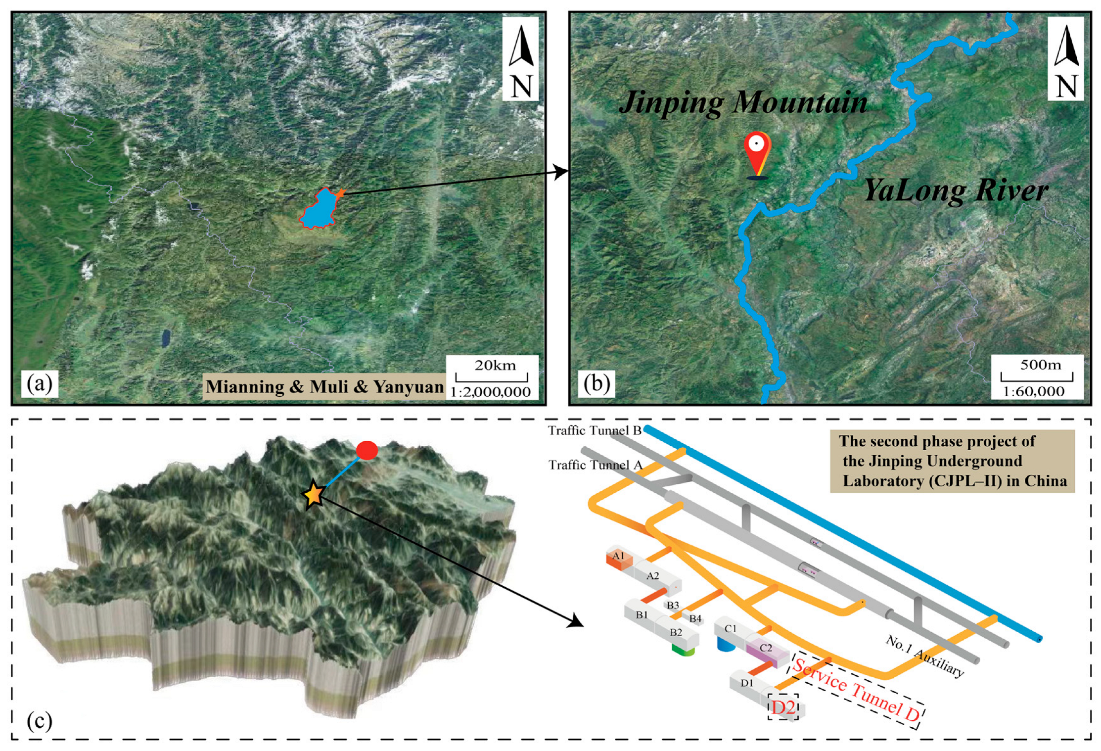
Figure 1. Introduction to the Jinping Underground Laboratory Project. (a) The locations of Mianning, Muli, and Yanyuan on the map; (b) The positions of Jinping Mountain and the Yalong River; (c) The specific location of the Jinping Underground Laboratory.
Buildings 15 03187 g001
Figure 2. Flow chart of the proposed CatBoost–SHGO algorithm.
Buildings 15 03187 g002
Figure 3. D2 laboratory numerical model. (a) A detailed introduction to the numerical model of the D2 laboratory; (b) The specific installation locations of the four sets of multi-point displacement meters; (c) The bare cavern of the D2 laboratory.
Buildings 15 03187 g003
Figure 4. Displacement training and testing of five points for 50 samples. (a) Training samples; (b) Testing samples.
Buildings 15 03187 g004
Figure 5. Parameter inversion comparison and displacement prediction comparison of five points. (a) Relative error of rock mass parameters; (b) Relative error of displacement.
Buildings 15 03187 g005
Figure 6. RFD and displacement cloud map under the feature excavation step.
Buildings 15 03187 g006
Figure 7. The relative error of the samples using CatBoost. (a) Training samples and (b) Testing samples.
Buildings 15 03187 g007
Figure 8. Distribution of inversion parameters in 28 steps of excavation.
Buildings 15 03187 g008
Figure 9. Comparison of inversion parameters under different excavation steps. (a) Tensile strength; (b) Elastic modulus; (c) Cohesion; (d) Internal friction angle.
Buildings 15 03187 g009
Figure 10. Comparison of inversion displacement of four boreholes with numerical simulation with field. (a) Borehole 1; (b) Borehole 2; (c) Borehole 3; (d) Borehole 4.
Buildings 15 03187 g010
Figure 11. Comparison of the inversion of four rock mass parameters of boreholes. (a) Tensile strength; (b) Elastic modulus; (c) Cohesion; (d) Internal friction angle.
Buildings 15 03187 g011
Figure 12. Comparison of inversion parameter accuracy and number of boreholes. (a) Tensile strength; (b) Elastic modulus; (c) Cohesion; (d) Internal friction angle.
Buildings 15 03187 g012
Figure 13. The inversion results within different parameter ranges. (a) Tensile strength; (b) Elastic modulus; (c) Cohesion; (d) Internal friction angle.
Buildings 15 03187 g013
Figure 14. Comparison of inversion parameters for four different parameter ranges.
Buildings 15 03187 g014
Figure 15. RFD cloud map comparison (inversion parameter value and initial value).
Buildings 15 03187 g015
Figure 16. Four rock mass parameters correlation graph (KDE).
Buildings 15 03187 g016
Figure 17. Four rock mass parameters sensitivity analysis.
Buildings 15 03187 g017
Figure 18. Optimal parameter E relative error diagram.
Buildings 15 03187 g018
Figure 19. Jinping Laboratory 3D safety monitoring system diagram.
Buildings 15 03187 g019
Figure 20. Displacement timing comparison and residual heat map. (a) Displacement heatmap; (b) Residual heatmap.
Buildings 15 03187 g020
Figure 21. On-site damage presentation. (a) The rock mass of the laboratory sidewall collapsed; (b) The lining of the ventilation pipe fell off.
Buildings 15 03187 g021
Table 1. Borehole No. 1 multi-point displacement meter data.
Excavation Step5 Monitoring Points on Multi-Point Displacement Meter
d1(mm)d2 (mm)d3 (mm)d4 (mm)d5 (mm)
11.4410.9630.3640.340.125
21.6211.1170.420.380.114
31.7311.4830.4250.3910.135
41.8461.5090.4380.3950.137
52.0421.7670.4560.4380.142
62.151.8350.6920.560.186
72.1912.050.7080.6320.21
82.2851.9580.7260.6630.231
92.5622.0460.7870.6810.231
102.6192.1510.870.7540.234
112.862.2690.9820.9480.282
123.6622.481.0440.9490.323
134.0872.5251.1841.0070.327
144.1822.5611.2141.0980.427
155.3992.7121.2181.1790.47
165.4542.9771.3591.3330.485
176.5973.9681.4671.3440.506
186.7094.3011.6261.4090.681
196.9344.3031.7371.4990.769
208.2144.521.7711.5890.794
218.3715.0171.8371.8141.129
228.4525.1962.0122.0921.281
2310.1015.2012.4822.1331.296
2411.0756.452.5872.51.826
2511.5576.762.682.8272.381
2611.8357.1563.2483.8072.534
2711.997.4033.5833.8782.679
2812.0887.5634.0343.9012.515
Table 2. D2 Statistics of rock mass parameters in the laboratory.
PropertiesTensile Strength
σ t / M P a
Yong’s Modulus
E / G P a
Cohesion
c / M P a
Internal Friction
φ / °
Value5.1 MPa40.522.727.4
Table 3. Inversion of the rock mechanics parameters.
PropertiesTensile Strength
σ t / M P a
Yong’s Modulus
E / G P a
Cohesion
c / M P a
Internal Friction
φ / °
Value4.75 MPa41.7420.8724.97
Table 4. The range of changes in four rock mass parameters.
Tensile Strength
σ t / M P a
Yong’s Modulus
E / G P a
Cohesion
c / M P a
Internal Friction
φ / °
Initial range[3.5, 6.0][35, 50][15, 30][20, 30]
Range 1[3.125, 6.375][25, 55][11.25, 33.75][17.5, 32.5]
Range 2[2.75, 6.75][20, 60][7.5, 37.5][15, 35]
Range 3[2.375, 7.125][15, 65][3.75, 41.25][12.5, 37.5]
Range 4[2, 7.5][10, 70][0, 45][10, 40]
Disclaimer/Publisher’s Note: The statements, opinions and data contained in all publications are solely those of the individual author(s) and contributor(s) and not of MDPI and/or the editor(s). MDPI and/or the editor(s) disclaim responsibility for any injury to people or property resulting from any ideas, methods, instructions or products referred to in the content.