Abstract
Unsafe events such as slips and trips occur regularly on construction sites. Efficient identification of these events can help protect workers from accidents and improve site safety. However, current detection methods rely on subjective reporting, which has several limitations. To address these limitations, this study presents a sound-based slip and trip classification method using wearable sound sensors and machine learning. Audio signals were recorded using a smartwatch during simulated slip and trip events. Various 1D and 2D features were extracted from the processed audio signals and used to train several classifiers. Three key findings are as follows: (1) The hybrid CNN-LSTM network achieved the highest classification accuracy of 0.966 with 2D MFCC features, while GMM-HMM achieved the highest accuracy of 0.918 with 1D sound features. (2) 1D MFCC features achieved an accuracy of 0.867, outperforming time- and frequency-domain 1D features. (3) MFCC images were the best 2D features for slip and trip classification. This study presents an objective method for detecting slip and trip events, thereby providing a complementary approach to manual assessments. Practically, the findings serve as a foundation for developing automated near-miss detection systems, identification of workers constantly vulnerable to unsafe events, and detection of unsafe and hazardous areas on construction sites.
1. Introduction
Slips and trips are common near-miss events on construction sites, which often trigger or precede severe fall accidents and injuries [1]. Despite the regular occurrence of these incidents, they are among the most unreported and undetected events on construction sites [2]. Studies suggest that approximately 20% of dangerous accidents, such as falls on construction sites, are triggered by near-miss incidents such as slips and trips [3,4]. However, research has reported that many slip and trip incidents go unreported due to factors such as worker reluctance, lack of systematic reporting systems, and low management priority, particularly since near-miss events often leave no tangible evidence unless they result in injury [5,6]. This substantial underreporting limits the accurate assessment and prevention of these hazardous events, making it challenging to address their root causes and prevent recurrence [7]. Effective detection of these incidents is important since it presents an opportunity to identify constantly vulnerable workers, hazardous areas on site, and other risk factors that trigger these incidents.
Traditional methods for detecting and documenting construction worker slip and trip incidents rely on subjective evaluations and manual monitoring by workers and supervisors [8]. While straightforward, this approach is inherently subjective, prone to underreporting, and dependent on individual perception and willingness to report events [9]. Also, near-miss incidents are especially vulnerable to omission during manual and subjective reporting, as they often leave no visible evidence and are perceived as less critical than actual accidents [10]. These shortcomings result in incomplete safety records, delayed hazard identification, and missed opportunities for preventive intervention. To address these limitations, two advanced methods, which include accelerometer-based monitoring using wearable inertial measurement units (IMUs) and computer vision-based techniques, have been explored. Studies have evaluated the potential of using IMUs to detect near-miss events, falls, and postural instability [4,11,12]. Although these prior studies have achieved good accuracy, the accelerometer and IMU devices, while portable, require constant calibration and are sensitive to environmental conditions such as temperature. These systems also only capture events in binary classification approaches [3]. Computer vision-based techniques have also been implemented for detecting slip and trip incidents. This method involves using devices such as closed-circuit televisions (CCTVs) to monitor construction sites to detect hazards and unsafe events [13]. Computer vision methods can be highly accurate in controlled conditions, but they are not suitable for continuous monitoring or specific worker detection and are hampered by occlusions, poor lighting, and restricted fields of view. This highlights the need for more effective methods [14].
Sound-based classification may present a more effective approach for slip and trip detection. It involves identifying events by recording and analyzing their associated sound patterns [15]. The rationale is that activities generate distinct sound patterns, and machine learning algorithms can leverage these unique patterns for classification. In contrast to the limitations of vision-based systems and IMU-based methods, the proposed sound recognition approach addresses these shortcomings by offering a low-cost and non-intrusive method that can operate effectively in visually obstructed areas and under varying environmental conditions. This method also offers an objective, automated, and continuous monitoring method that captures the unique acoustic signatures of slip and trip events in real time. This eliminates reliance on self-reporting, ensures consistent detection even in the absence of witnesses, and provides reliable data for proactive safety management. Several construction studies have explored sound-based classification for tasks such as estimating cycle times of construction operations, identifying equipment on sites, and detecting pipelines and scaffold damage [16,17,18]. However, despite the high accuracies achieved in various studies, sound signals have not been fully explored for personalized worker monitoring and the detection of unsafe incidents.
Therefore, this study evaluates the use of sound signals from a wearable sensor for slip and trip detection. While IMUs and vision-based systems have been widely studied, these devices come with limitations, including privacy infringement and environmental constraints such as poor visibility, changing temperatures, and inadequate line of sight. This study explores an alternative approach using wearable sound sensors, which are low-cost, non-intrusive, and capable of detecting subtle slip and trip near-miss events in real time, especially in varying environmental and visual conditions where visual or IMU data may be insufficient. Additionally, rather than classifying falls directly, this study focuses on detecting events such as slips and trips. This is because these incidents mostly precede fall accidents and are the key triggers of dangerous fall events [19]. To achieve the aim of this study, slip and trip events are simulated while a wearable sensor records the unique sound patterns associated with these events. Then, the recorded sound data are preprocessed, features are extracted, and several machine learning algorithms and deep learning models are trained. Practically, this study presents an effective method for detecting slip and trip incidents on construction sites. Construction and safety managers can leverage this objective detection system to automatically document such events for safety evaluations, identify workers who are consistently vulnerable to these incidents, and identify hazardous site conditions where slip and trip events frequently occur.
2. Literature Review
2.1. Acceleration-Based Workers’ Behavior Classification
The limitations of traditional site monitoring and the inefficiency of manual construction worker supervision have led researchers to explore more advanced monitoring techniques. Notable among these advanced methods is the assessment of physical responses. These techniques involve the use of devices composed of inertial measurement units (IMUs) to evaluate workers’ gait parameters and detect abnormal movements [20]. These devices have seen an increase in adoption due to their light weight, high portability, and affordability. Numerous research studies have been carried out to monitor human movement and activities using wearable IMU systems [21,22,23]. Studies have also demonstrated the potential of utilizing a single and multiple IMU devices to effectively evaluate human movements and events such as postural sway, gait analysis, and fall risk assessment [24,25,26,27]. These studies have also investigated the effects of factors, such as sensor placement, number of subjects, subjects’ gender, and signal processing methods, on the monitoring performance. In the construction industry, laboratory tests have successfully validated accelerometers for the detection of near-miss occurrences, fall hazards, and awkward postures. A study by Dzeng et al. [28] employed a smartphone with an IMU for falls and portent detection. The study achieved high accuracies ranging from 79% to 89.17%. Yang et al. [4,20] also presented automated methods for identifying and documenting near-miss falls and actual fall incidents by combining kinematic data obtained from wearable inertial measurement units (wIMUs) with various algorithms, including a one-class Support Vector Machine. The studies achieved promising accuracies and revealed a significant association between gait abnormality scores and fall hazards. Empirical studies show that the bias instability of MEMS-based IMUs is significantly influenced by ambient temperature. For instance, low-cost MEMS gyroscopes typically exhibit a bias temperature sensitivity on the order of ~500°/h per °C [29]. After appropriate calibration, whether via software modeling or turntable-based characterization, drift can often be suppressed with an over 70% reduction in RMS error. More recently, Lee et al. [30] presented an IMU-based method for detecting slip and trip-related fall risk incidents. The study utilized a graph-based approach where time-series based IMU data were converted into graph structure to present an opportunity for more generalization of the model across unseen data. The study achieved a correlation score of 0.95 between IMU features and slip- and trip-related behaviors. Yuhai et al. [31] also presented a deep learning-based method for slip–trip fall detection in construction. Simulated slips and trips were conducted, while body movement data were recorded using a waist-attached wearable device embedded with a single IMU sensor. By extracting 30 features and transforming them using bicubic interpolation, a LeNET-5 CNN was trained, and an accuracy of 90.39% was achieved. Park et al. [32] recently developed a novel miniaturized IMU sensor combined, which can be simultaneously attached to multiple body parts of workers for effective detection of worker behavior and near-miss events. The system automatically processes worker data using extended Kalman filters, and the experimental results reveal high accuracies of over 90% in detecting worker behaviors.
While several studies have demonstrated the use and efficiency of physical response assessments and IMUs for worker monitoring and unsafe behavior detection, these devices and methods have some limitations. First, workers have varying abilities to control their physical movements, and not all workers may exhibit abnormal patterns when they encounter hazards or conditions such as slips and trips [33]. Therefore, differences in physical response patterns may compromise the performance and generalizability of IMU-based methods. Second, devices such as IMUs are sensitive to environmental changes such as temperature and humidity, which may render them inefficient in construction sites that possess varying environmental conditions [34].
2.2. Computer Vision-Based Workers’ Behavior Classification
Computer vision-based techniques have also been explored for worker monitoring and detection of unsafe events. These methods involve the use of systems such as CCTV cameras to monitor construction sites and identify abnormal behaviors [35]. Several studies have presented vision-based methods due to the advantages these techniques present for site monitoring. Han et al. [36] proposed an unsafe behavior monitoring system using a vision-based detection method. The proposed method showed promising results in identifying predefined unsafe events for workers using ladders. In a follow-up study by Han et al. [37], the authors proposed an enhanced model that combined a comprehensive analysis of various fall-related body motion features such as rotation and joint angles, significantly enhancing performance. Computer vision was also applied for automated PPE inspection by Fang et al. [38]. A deep learning-based occlusion mitigation method was presented, and it proved robust under varying lighting conditions, individual differences, window types, and partial occlusions. Ding et al. [39] developed a deep hybrid model combining CNN and LSTM to automatically detect unsafe ladder-climbing behaviors. The model accurately classified worker actions as safe or unsafe, achieving 92% accuracy across four action categories. Additionally, Lee et al. [40] introduced a computer vision model that leverages a combination of synthetic and real-world datasets for automated safety monitoring in construction sites. The validation outcomes revealed a significant enhancement in the detection rate of small-sized personal protective equipment worn by construction workers, surpassing a 30% improvement compared to the prior method that relied solely on single-source data. In a recent study, Bonyani et al. [41] presented an advanced vision-based method for construction worker unsafe event monitoring and activity detection. The study introduced an optimized positioning (OP-NET) architecture with an attention-based spatiotemporal sampling approach to enhance vision-based detection. By evaluating the proposed system on an existing image dataset including CMA and SODA, high accuracies were achieved, demonstrating the ability of the proposed system in worker unsafe action detection.
Although computer vision-based methods have proven to be robust in detecting unsafe behaviors under decent light conditions, these methods may face challenges in conditions with poor lighting and inadequate line of sight. Also, these techniques only capture workers within specified visual ranges, making them unsuitable for continuous worker monitoring and detection of abnormal occurrences such as slips and trips in areas not covered by the field of view.
2.3. Sound-Based Applications in the Construction Industry
Sound-based assessment may present an effective opportunity to monitor construction workers’ behavior and identify occurrences such as slips and trips. The sounds and noises generated from workers’ activity and equipment operations provide critical insights on task performance and safety issues [42]. Although the application of sound-based classification in construction has been explored to some extent, the current sound-based assessment methods have mainly focused on equipment operations and other dimensions, such as the assessment of modular construction activities. Several studies have been undertaken to explore the applicability of sound data in estimating cycle times of construction operations, recognizing construction equipment activity, and detecting construction damage on pipelines and scaffolds [17,18,43,44]. For instance, Sabillon et al. [43] proposed a method for predicting construction cycle times using audio data from cyclic activities. By applying Bayesian analysis, they developed predictive models linking audio features to specific tasks, achieving over 90% prediction accuracy in preliminary tests. Cheng et al. [17] developed an audio-based system for analyzing and tracking heavy equipment activities on construction sites, achieving accuracies exceeding 80% with SVM. Sherafat et al. [18] introduced a CNN-based method for identifying activities of different construction equipment. A novel data augmentation method was implemented to simulate real-world sound mixtures during simultaneous activities, achieving accuracy above 70%. Rashid and Louis [45] developed a method to recognize construction workers’ manual activities in modular factories by training models on sounds like hammering, nailing, and sawing. Their approach achieved 93.6% classification accuracy, with cepstral-domain features proving most effective for sound classification. A study by Mannem et al. [46] also presented a sound-based method for detecting various construction activities. By utilizing a hybrid CNN-LSTM model and MFCCs-LSTM architecture, audio data recorded from real-time closed environments were used to train the models, achieving an overall precision of 89%.
In terms of worker safety monitoring using sound, very limited studies have been conducted in the construction industry. However, few studies have explored sound data to monitor individual health and events such as falls in other industries, such as health. Collado-Villaverde et al. [47] proposed a machine learning method for detecting falls of elderly people using sound. By simulating fall events and extracting frequency-domain features such as zero-crossing rate and spectral centroid, machine learning algorithms were trained, and high accuracies of 87.5% were achieved. In another study, Kaur et al. [48] developed a transformer-based approach for detecting elderly fall accidents using sound, which achieved an accuracy of 86.7%. Other studies have also explored other machine learning and deep learning models, such as decision trees and CNN, in detecting falls in elderly persons [49], achieving acceptable accuracies above 93%. Despite the potential utilization of sound and machine learning algorithms for individual safety monitoring, especially for detecting slips and falls, this method has not been explored for worker safety monitoring in construction.
2.4. Research Gaps and Hypotheses
From the above review of the literature, two main research gaps were identified.
- 1.
- Current slip and trip methods rely on physical responses and computer vision, which have limitations.
Existing studies have proposed objective methods for detecting unsafe events such as slips and trips, primarily relying on inertial measurement units (IMUs) and computer vision-based techniques. However, these methods face several limitations, including sensor placement constraints, occlusions with vision-based approaches, and potential inaccuracies in complex construction environments. Alternative methods are required to enhance detection capabilities and complement existing techniques. This study investigates sound-based monitoring as a novel approach for detecting unsafe events such as slips and trips in construction.
- 2.
- No study has explored the use of sound-based classification for construction worker safety assessment and detection of unsafe events.
Sound-based classification research in construction has primarily focused on equipment monitoring, manual task identification, and damage detection. While sound-based monitoring has been explored in healthcare for detecting falls in elderly populations with promising results, its application in construction safety, particularly for detecting unsafe events such as slips and trips, remains unexplored. This study addresses this gap by evaluating the feasibility of utilizing wearable audio sensors for slip and trip detection among construction workers
To address the above research gaps, this study explores the potential of detecting slip and trip events using audio recorded from a wearable device. Based on the review of the sound-based classification literature, the following hypotheses are proposed.
H1.
Machine learning models trained on audio features will achieve high accuracies in detecting slip and trip events.
Previous studies [47,48] in other domains have demonstrated that unusual events such as falls generate distinct acoustic patterns that differ from patterns associated with normal walking and movements. Therefore, it is expected that slip and trip events in this study will generate unique acoustic patterns, which will enable models to learn effectively and achieve high accuracies in differentiating between slips, trips, and normal events.
H2.
Image-based (2D) sound features will outperform 1D features in slip and trip classification.
Features from audio signals can be represented in 1D and 2D formats. However, some previous studies have found that 2D sound representations, such as MFCC spectrograms, are more robust in various sound-based classification tasks, including equipment monitoring and manual activity detection [43,50]. This superior performance has been attributed to the capabilities of 2D features to capture temporal and spectral relationships, thereby providing a more comprehensive representation of the acoustic patterns of sound [51]. Therefore, 2D features are expected to yield higher detection accuracies for slip and trip detection compared to 1D features.
3. Methodology
Figure 1 shows the overall process for sound-based slip and trip classification. The process consists of four key steps: (1) data collection, (2) data processing, (3) machine learning classification, and (4) deep learning classification. In Step 1, slip and trip events were simulated, and the corresponding sounds were recorded using a smartwatch. In Step 2, the recorded data were labeled into 3 categories: normal walking, slips, and trips. Data augmentation processes were then applied to expand the dataset and increase feature diversity. In Step 3, relevant time-series features were extracted from the recorded sound signals, and machine learning models were trained. In Step 4, 2D image features were extracted from the audio data and used to train various deep learning models.
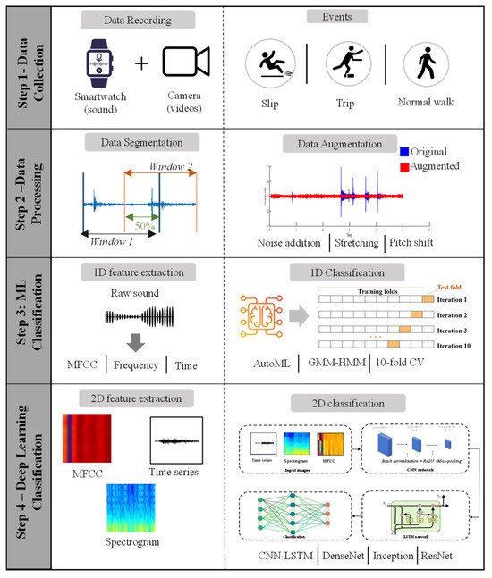
Figure 1.
Overall process for sound-based slip and trip classification.
3.1. Data Collection and Participants
Figure 2 shows the experimental setup for data collection and the types of simulated events. Slip and trip events were simulated in a controlled laboratory setting due to the limited availability of datasets online. The recordings were captured using the built-in digital microphone of the Apple Watch Series 6, which offers an approximate frequency response of 20 Hz–20 kHz and was configured at a sampling rate of 44.1 kHz and a precision of 16-bit. The choice of a 44.1 kHz sampling rate and 16-bit precision in most audio research originates from the Compact Disc (CD) standard, which was developed to balance fidelity, storage efficiency, and compatibility across devices. The 44.1 kHz rate exceeds the Nyquist–Shannon theorem’s minimum requirement of twice the highest audible frequency (~20 kHz), providing headroom for anti-aliasing filtering while fully capturing the human hearing range [52,53]. The 16-bit depth offers a theoretical dynamic range of approximately 96 dB, sufficient to encompass the quietest to loudest sounds perceivable by humans while keeping quantization noise low [54]. The widespread adoption of these parameters in research is attributed to their compatibility across audio devices, accessibility in existing datasets, and suitability for diverse applications in speech, music, and psychoacoustic analysis [55]. In addition to audio recording, videos were recorded to assist in data labeling. The subjects in this study were 10 health students and staff of PolyU (7 males and 3 females) with ages ranging from 28 to 42 years (mean 33.4 ± 5.4 years). Subjects had heights ranging from 1.66 to 1.83 m (mean 1.7 ± 0.1 m), weights ranging between 59 and 85 kg (mean 68.8 ± 9.9 kg), and varying work experience ranging from 2.5 to 13 years (mean 6.9 ± 4 years). The selected subjects had no history of injuries to the upper extremities, lower back, and lower extremities, as well as neurological disorders, that could impact body balance function. The experiment was designed safely to prevent injuries, and subjects were well trained based on representative videos. Necessary safety gear was provided, and all subjects provided written consent.
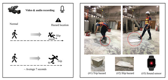
Figure 2.
Experimental setup for data collection.
To effectively simulate slip and trip events, low-density polyethylene was placed on the walking paths of subjects to trigger slip events, while a concrete block was also placed along the subjects’ trajectory to induce trip events. During the testing session, subjects were required to traverse a designated path at their own pace, while keeping their gaze straight ahead so as not to anticipate the presence of unsafe surface conditions. Each participant performed 25 repeated trials of slips and trips, with each trial averaging 7 seconds (5.5 seconds for walking plus an additional 1.5 seconds to simulate the slip or trip behavior). Each subject performed 25 repeated trials, as this dataset quantity provided adequate data points for model training, as indicated by some studies [45].
3.2. Data Labeling, Augmentation, and Segmentation
3.2.1. Data Labeling
The recorded sound data were manually labeled into three categories (normal walking, slip, and trip). The labeling was conducted using the recorded videos and by observing the amplitude of the recorded sounds. Figure 3 shows examples of labeled sound sensor data. In Figure 3, the vertical axis represents the raw signal amplitude, which was normalized to the range of −1 to 1 by dividing the waveform by its maximum absolute value, solely for visualization and labeling purposes. The subsequent analysis is not only based on these raw amplitudes; instead, the acoustic features (e.g., MFCCs) used for model training are described in Section 3.3 and Section 3.4. Each event category generated unique signal patterns. For instance, during walking, low-frequency cyclic sound patterns were generated. On the other hand, distinct abnormal sound patterns were produced for slip and trip events. The slip events generated a relatively long time-series trend but with low energy (Figure 3a) because they resulted from the foot slipping forward against the floor. In contrast, during a trip event, an initial impulsive peak was generated when the subject’s foot struck an object, followed by another higher peak as the subject fell and collided with the ground (Figure 3b). Both slip and trip events also had a peak point for recovering body balance before returning to normal walking.
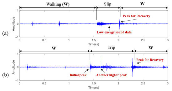
Figure 3.
Labeled sound sensor data in the time domain: (a) slip; (b) trip.
3.2.2. Data Augmentation
Characteristics such as participants’ weights, body orientation, and nature of landing can influence the impact force against the floor, which results in diverse sound features [56]. Additionally, on-site recorded sounds may possess varying noise interference, which may affect the recorded slip and trip sounds. To account for this, data augmentation was conducted. Data augmentation of audio signals using time stretching, pitch shifting, and noise addition is a widely adopted and standard practice in audio and speech processing tasks (e.g., sound event detection, speech recognition, and music information retrieval) [57,58]. By implementing data augmentation to the dataset, the model is exposed to a wider range of sound variations. This improves its ability to generalize to unseen conditions and reduces overfitting to the limited original recordings. Figure 4 shows five data augmentation techniques conducted to improve sound diversity and data size. In the first method, the duration of each sound clip in the dataset was instantly increased by a factor of 1.20. In the second augmentation method (slowly stretching the time), the time stretching factor was applied to slow down the recorded sounds by a factor of 0.80. Positive pitch shift involved increasing the pitch of each audio signal by a positive factor of 1.2, which led to a change in the pitch of the audio data. Therefore, the representations for pitch shifting were illustrated using frequency instead of time, as shown in Figure 4c. The negative pitch shift involved decreasing the pitch of the deformed dataset by a factor of −0.8 after the pitch-shifting process. Furthermore, on-site recordings inevitably contain different background noises. For the noise addition, two different construction background noises with varying equipment sounds were introduced into the original sound data. After conducting data augmentation, 1500 audio clips, including the 250 original clips and 1250 augmented clips, were utilized for training. Since the sound sensor’s sensitivity value often influences the sound signal’s output, the sound data were normalized within a range of −1 to 1 to mitigate the impact of sound sensitivity [59].
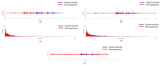
Figure 4.
Data augmentation techniques: (a) quickly stretching the time, (b) slowly stretching the time, (c) positive pitch shift, (d) negative pitch shift, (e) white noise.
3.2.3. Data Segmentation
Sound data in their raw form often pose challenges for traditional supervised algorithms due to the inherent sequential nature of the data [60]. Therefore, conducting data segmentation is crucial to transform sequential supervised learning problems into traditional supervised learning problems [61]. In this study, the raw sequential audio was segmented into shorter signals using a sliding window approach. The windowing process treats the typically non-stationary sound signal as quasi-stationary within each window, facilitating the classification of segmented data within individual windows using conventional supervised learning [62]. From previous studies [63], it was noted that using frequency-domain features requires the number of audio samples within each window to be a power of two (2n). In this study, five different numbers of audio samples within each window were first selected as 2048 (211), 4096 (212), 8192 (213), 16,384 (214), and 32,768 (215). Then, the corresponding distinctive window sizes were calculated using the number of audio samples within each window and the number of audio samples per second, as shown in Equation (1). Here, the number of audio samples per second is a consistent value of 44,100 since the recording frequency was set to 44.1 kHz. Therefore, five distinct window sizes of 0.046 s, 0.093 s, 0.186 s, 0.372 s, and 0.743 s were selected, with an overlap of 0.5 according to the methodologies of some previous studies [51]. The 50% overlap was chosen because it reduces the risk of missing transient events at frame boundaries. Furthermore, based on primary tests with different overlap ratios (25%, 50%, 75%), a 50% overlap provides a good balance between temporal resolution and computational cost, avoiding excessive redundancy while ensuring that important signal details are preserved.
Table 1 shows the total number of window segments obtained from the collected 1500 recorded audio clips with varying window sizes. It can be identified that as the window size doubles, the corresponding number of window segments decreases by around half. After data segmentation, each window segment was assigned one of three labels (normal, slip, trip). If the area covered by the window encompassed over 50% of either ‘slip’ or ‘trip,’ the window segment was labeled as either ‘slip’ or ‘trip.’ All other window segments were labeled as ‘walking’. Figure 5 illustrates an example of data labeling for window segments. The ‘walking’ sound signal is highlighted in a dashed orange box, while slip or trip events are highlighted in solid green boxes. The left window segment highlighted in green is labeled as a ‘trip’ behavior since 70% of its area corresponds to the trip signal. Conversely, the dashed orange window segment located on the right side is labeled as ‘walking’ because only 24% of the trip sound signal falls within that window.

Table 1.
Number of window segments from the 1500 recorded audio clips.
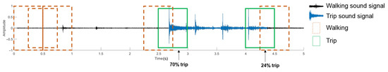
Figure 5.
Data labeling for window segments.
3.3. One-Dimensional (1D) Feature Extraction and Sound Classification Using Machine Learning
Table 2 shows the 1D features extracted from process audio signals. Features are defined as the extracted values and dimensions of raw or converted signals that contain unique and more understandable patterns compared to raw datasets [64]. Raw sound data often contain redundant or irrelevant information. Therefore, feature extraction is important to transform the raw audio into a more representative format. Several feature categories have been used in previous studies [17,18,45,51], and the most predominant features include the time domain, frequency domain, and Mel-frequency cepstral coefficient (MFCC) features. Time-domain features are defined as the extracted values based on the amplitude of the sound signal, which are typically measured in decibels (dB) at regular intervals over time [18]. Frequency-domain features, which refer to the characteristics of signals derived from their frequency contents, were also extracted [65]. The third feature category was the MFCC. MFCC features present spectral characteristics of the audio signal, which are robust to variations in background noise and other factors that can affect the acoustic properties of the signal [66]. They are derived from analyzing the frequency content of sound data. A total of ten time-domain features, five frequency-domain features, and 13 MFCC features were extracted according to the methodologies of previous sound-based studies. The first 13 MFCC features were considered because they have been found to contain most of the relevant information necessary for sound classification [67].
Table 2.
One-dimensional (1D) features extracted from the processed audio signals.
After feature extraction, several machine learning algorithms were trained to classify the 1D sound features into three classes of events. In the current work, no manually assigned weighting factors were introduced. Instead, a machine learning model was employed to take all extracted features as input. The relative importance of each feature was learned automatically during model training, allowing the feature selection and weighting process to be driven by data rather than predefined heuristics.
According to some prior studies [68], Hidden Markov Models–Gaussian Mixture Models (HMM-GMM) and Support Vector Machines (SVMs) are the most robust in sound classification based on 1D feature types. However, since classifier performance varies based on recorded data and other experimental features, it is necessary to assess the performance of various classifiers to determine the most suitable algorithm for the current dataset [42]. Therefore, in this study, 15 machine learning models were trained using an automated machine learning (AutoML) approach, and an additional HMM-GMM was also trained. AutoML is a machine learning system that simultaneously automates the machine learning process by handling tasks such as hyperparameter tuning for several classifiers [69]. The datasets were split into a 70/30 train–test ratio, and a 10-fold cross-validation technique with a random search strategy was applied for training and hyperparameter tuning on the 70% data, while testing was conducted on an independent 30% dataset. The 10-fold cross-validation technique is a commonly used method for model training and hyperparameter tuning, and it ensures optimal model performance. A random search strategy was implemented to find the most effective hyperparameters.
In addition to the 15 AutoML models, a custom GMM-HMM model was also trained. Despite being old, this model has demonstrated strong robustness in sound-based classification in previous studies. Figure 6 shows a schematic layout of the GMM-HMM. The HMM is designed to predict hidden states based on the sequences of prior hidden states and observable features by computing transition and emission probabilities [70]. In this study, the hidden states correspond to the behavior labels—walking, slips, and trips—while the observable nodes are derived from extracted sound signal characteristics modeled using the GMM. The use of GMM presents some advantages since it prevents the performance reduction that can occur when directly using time-series features [71].
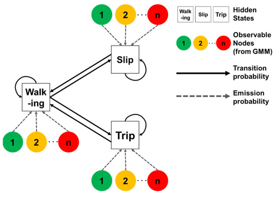
Figure 6.
Schematic illustration of the GMM-HMM used in this study.
3.4. Image-Based (2D) Feature Extraction and Sound Classification Using Machine Learning
Three 2D image feature categories, which include (1) spectrogram images, (2) time-series images, and (3) MFCC images, were extracted to train the deep learning models. These features effectively represent sound properties in visual formats [18,43]. Figure 7 shows the feature images extracted from sound data. The time-series images were generated by plotting the amplitude of segmented raw audio data along the time series (Figure 7a). Spectrogram images were also extracted because they effectively model the temporal and spectral characteristics of the sound [72]. The spectrogram images were generated in 128 × 128 pixels because this size presents an opportunity for deep neural networks to learn the unique patterns of sound [73]. In addition, MFCC images were also extracted due to their robustness in representing audio signals very distinctively [66]. To extract the MFCC images, each segmented sound datum was divided into 14 frames with an overlap of 50%. Then, the first 14 MFCC coefficients were extracted from each frame to create 14 × 14 MFCC images.
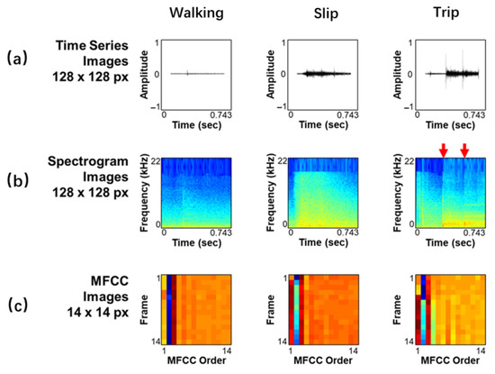
Figure 7.
Image features extracted from the sound data: (a) time series; (b) spectrograms; (c) MFCC.
After extracting 2D image features, several deep learning models were trained. Two custom-trained networks, which include a CNN and a hybrid CNN-LSTM network, were trained. Figure 8 shows the proposed hybrid CNN-LSTM deep learning architecture. The reason for using this hybrid model is because of the high robustness of CNN models in image classification, as well as the capabilities of LSTM networks to learn temporal dynamics in tasks such as speech recognition and sound analysis [74]. Additionally, compared to using other models such as LSTM or GRU alone, the CNN-LSTM architecture offers more efficient feature extraction by employing convolutional layers to reduce the dimensionality of raw inputs prior to temporal sequence modeling. This integration often results in improved predictive performance and reduced training complexity, particularly for high-dimensional time–frequency representations [75,76]. While transformer-based architecture has demonstrated strong performance in various audio processing tasks [77], they generally require substantially larger datasets and greater computational resources, which were beyond the scope of this proof-of-concept study. Traditional machine learning methods such as Support Vector Machines (SVMs) or Random Forests were also considered; however, these approaches tend to underperform on high-dimensional time–frequency data unless supported by extensive handcrafted feature engineering [78,79]. The CNN-LSTM model comprised three convolutional layers with a kernel size of 3 × 3, followed by a Long Short-Term Memory (LSTM) layer with 128 units to capture temporal dependencies. Training was performed for up to 100 epochs with early stopping (patience = 10), using a batch size of 64. The learning rate was set to 0.001, and optimization was carried out using the Adam optimizer. This configuration was selected to balance model complexity with generalization performance and ensure reproducibility.
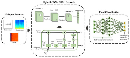
Figure 8.
Proposed hybrid CNN-LSTM deep learning architecture.
In addition to the custom-trained CNN and CNN-LSTM, four pre-trained networks, which include InceptionV3, ResNet50, InceptionResNetV2, and DenseNet169 [80,81,82], were also tested using a transfer learning approach. This was done to evaluate their performance in sound classification and to serve as base comparison models for the custom-trained CNN and hybrid CNN-LSTM models in this study.
4. Results
4.1. Results of Slip and Trip Classification Based on 1D Features Using Machine Learning
This section presents the classification performance of machine learning algorithms in slip and trip detection. Additionally, insights related to the impact of window sizes and feature categories are discussed.
4.1.1. Performance of Machine Learning Algorithms in Slip and Trip Classification Based on 1D Features
The elected hyperparameters for various classifiers are provided in Appendix A. Table 3 presents the overall performance of various machine learning classifiers in sound-based slip and trip classification using the smallest window size. Some key findings can be noted from the table. First, the results show that the GMM-HMM outperforms all other models, achieving the highest accuracy (0.918) and F1 score (0.920). This superior performance is consistent with previous studies where this dual model has been found to outperform other traditional machine learning classifiers in sound classification tasks [83]. This performance can be attributed to the hybrid nature of the GMM-HMM, which integrates both temporal and spectral information [84]. Second, most models achieved an accuracy above 0.86, with only small performance variations among the top performers. This indicates that slip and trip detection based on sound is well suited to a range of ML approaches, although sequential models such as GMM-HMM demonstrate greater robustness. Third, other performance metrics including F1 score, recall, and precision remained high across most classifiers, suggesting balanced performance with low rates of misclassification.
Table 3.
Overall performance of machine learning classifiers in sound-based slip and trip classification.
Table 4 presents the test performance of machine learning classifiers across varying window sizes. The table shows three key findings. First, although the GMM-HMM model achieved the highest accuracy of 0.918 in the smallest window, its average accuracy across the five window sizes was 0.856. This suggests that while the GMM-HMM model is highly effective in smaller window sizes, its performance declines significantly with increasing window sizes. According to Dahl et al. [85], although GMM-HMM models can initially achieve competitive performance, they are susceptible to performance degradation when large or suboptimal window sizes are selected. Second, tree-based and boosting algorithms such as CatBoost, LightGBM, and gradient-boosting machines performed better than traditional classifiers such as decision trees and Random Forests. Notably, CatBoost and LightGBM both achieved an accuracy of 0.907 in the smallest window. This finding aligns with previous studies, where these algorithms have consistently outperformed conventional machine learning classifiers [86]. Gradient-boosting models, such as CatBoost, incorporate mechanisms such as inbuilt boosting enhancement, which help mitigate data bias and variance and lead to superior performance [87].
Table 4.
Test performance of machine learning classifiers across varying window sizes.
4.1.2. Performance of Various 1D Feature Categories in Slip and Trip Classification
Table 5 shows the classification performance of different feature categories in slip and trip detection. Three key findings can be noted from the table. First, MFCC features outperformed the other feature categories across all algorithms, achieving an average accuracy of 0.867, compared to 0.795 and 0.779 for frequency- and time-domain features, respectively. This finding aligns with previous studies, where MFCC features were more effective compared to other features [88]. The superior performance of MFCC coefficients can be attributed to their ability to effectively represent unique sound patterns while filtering out redundant ones [89]. Second, combining all feature categories resulted in the highest classification accuracies across most models, with an average accuracy of 0.873. This improvement is likely due to the model’s ability to learn from diverse feature sources. Previous studies have shown that integrating multiple feature types enhances machine learning performance since models leverage the strengths of each category [90]. The combination of time-domain, frequency-domain, and MFCC features allowed models to capture a broader range of temporal, spectral, and cepstral characteristics, leading to more robust performance. Third, although combining all features generally yielded higher classification accuracy, some classifiers produced different results. For instance, in the QDA algorithm, MFCC features achieved an accuracy of 0.849, outperforming the 0.791 accuracy obtained when all three feature categories were combined. The Naïve Bayes algorithm also showed a similar trend. This performance decline may be attributed to the high-dimensional nature of the data when all feature types were combined. According to Wibowo et al. [91], algorithms such as Naïve Bayes prioritize simplicity and computational efficiency, which can result in suboptimal performance when dealing with high-dimensional feature spaces or datasets with many features.
Table 5.
Classification performance of various 1D feature categories.
4.2. Results of Slip and Trip Classification Based on 2D Features Using Machine Learning
The three features extracted, which include (1) MFCC images, (2) spectrogram images, and (3) time-series images, were used to train several models, including CNN, LSTM, and hybrid CNNLSTM classifiers. In addition, four pre-trained models were also tested using a transfer learning approach. This section presents the findings of the deep learning networks in slip and trip classification using image features.
4.2.1. Performance of CNN and CNN-LSTM Models in 2D Image-Based Slip and Trip Classification
Table 6 shows slip and trip classification accuracies of the deep learning algorithms using various image features across different windows. From the table, three key findings can be noted. First, the dual CNN-LSTM algorithm outperformed other models, achieving the highest average accuracy of 0.949 when the MFCC features were used. Second, all CNN-LSTM models achieved higher accuracies compared to the traditional CNN models. The CNN-LSTM trained with time-series images and the CNN-LSTM-trained spectrogram images performed well, with accuracies of 0.924 and 0.906, respectively. These findings highlight the effectiveness of integrating convolutional and sequential learning models for sound-based slip and trip classification. Third, the impact of increasing window size on model performance varied across models and feature categories. While some models showed improved performance, others exhibited a slight decline in accuracy. For instance, the CNN model using spectrogram image features showed a steady increase in accuracy, rising from 0.807 at the smallest window size (0.046 s) to 0.862 at the largest window size (0.743 s). However, other models, particularly the CNN-LSTM model using MFCC features and spectrograms, experienced a slight decline in accuracy as the window size increased. This finding suggests that while certain models can effectively capture slip and trip patterns in sound regardless of window size, others may experience performance degradation. This underscores the importance of selecting an optimal window size.
Table 6.
Slip and trip classification accuracies of CNN and CNN-LSTM models using various image features.
4.2.2. Performance of Various Pre-Trained Models in 2D Image-Based Slip and Trip Classification
Figure 9 shows the average performance of the pre-trained models across five window sizes and their classification performance using different image feature types. The figure presents four key findings. First, spectrogram-based models achieved the highest average accuracy of 84.1%, outperforming MFCC and time-series-based models. This contrasts with the findings from the hybrid CNN-LSTM model, where MFCC features outperformed spectrogram and time-series images. Second, spectrogram-based models exhibited significant performance variation across different architectures despite their high average accuracy. Notably, ResNet50, with spectrogram features, recorded the lowest accuracy of 75.5%. This suggests that the performance of spectrogram image features is highly dependent on the neural network, with some models better suited for spectral features compared to others. Third, DenseNet169 was the best-performing model across all feature categories, achieving the highest accuracy of 87.9% when spectrogram features were used. This superior performance can be attributed to its dense connectivity pattern, where each layer receives inputs from all preceding layers [82]. This enhances the flow of information and gradients throughout the network, facilitating more effective training [92]. Fourth, time-series-based models recorded the lowest overall classification performance, with accuracies of 80.5% in ResNet50 to 84.7% in DenseNet169. The low performance of time-series features, compared to spectrograms and MFCC features, suggests that raw sound signal images may not contain sufficiently distinctive patterns to effectively classify slip and trip events. However, their moderate performance indicates that they remain a viable alternative, particularly in conditions where computational efficiency is a priority, since these features are easy to extract and do not require conversions into the frequency domain.
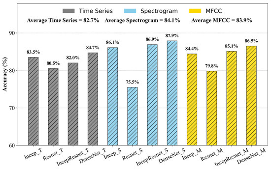
Figure 9.
Average performance of the pre-trained models across five window sizes and their classification performance using different image feature representations.
Table 7 shows the performance of pre-trained models using various image features across different window sizes. Two key findings emerge from the results. First, shorter window sizes (0.046 s and 0.093 s) generally resulted in higher classification accuracies across most models, whereas longer window sizes (0.372 s and 0.743 s) led to performance declines. This trend is particularly evident in the ResNet50 model with MFCC features, where accuracy dropped significantly from 0.851 in the 0.046 s window to 0.719 in the 0.743 s window, a decrease of over 13%. Similarly, the InceptionV3 model with time-series images gradually declined in performance, decreasing from 0.844 to 0.821. Similar performance reductions were observed in ResNet50 and InceptionV3 when trained with MFCC features. These findings suggest that larger window sizes may introduce noise or redundant information, diminishing classification effectiveness. Second, while most models exhibited a decline in performance with increasing window size, certain models demonstrated high stability across different window sizes, indicating their robustness to window variations. For instance, the DenseNet169 model trained with time-series images exhibited the lowest standard deviation (0.002), maintaining nearly constant accuracy across all window sizes. Similarly, the DenseNet169 model with spectrogram images and the InceptionResNetV2 model trained with MFCC features showed minimal accuracy fluctuations, suggesting that these models effectively manage variations in window size without significant performance degradation.
Table 7.
Performance of pre-trained models using various image features across various windows.
5. Discussion
5.1. Comparison of Machine and Deep Learning 1D Classification Performance
Deep learning algorithms were implemented in this study mainly to evaluate the effectiveness of various image-based (2D) features in slip and trip classification. However, given that deep learning architectures also perform well in 1D classification tasks, it was necessary to assess their performance in 1D sound-based slip and trip classification and compare them with machine learning classifiers. To this end, three deep learning architectures—Bidirectional Long Short-Term Memory (Bi-LSTM), One-Dimensional Convolutional Neural Networks (1D-CNNs), and Long Short-Term Memory (LSTM)—were trained. These models were selected due to their proven effectiveness in previous 1D and time-series classification studies. To ensure a fair comparison with machine learning models, the datasets were divided using a 70/30 train–test split, with 70% allocated for training and 30% for testing. Hyperparameter optimization was also conducted using a 10-fold cross-validation approach and a random search technique with various hyperparameter configurations, including epoch, batch size, learning rate, and dropout rate, systematically tested to determine the optimal combination for each model.
Table 8 shows the classification performance of the three deep learning models. From the table, two key findings can be noted. First, the Bi-LSTM model demonstrated the highest performance across the five window sizes, achieving an average accuracy of 0.894, while the LSTM model exhibited comparable performance with an average accuracy of 0.893. The 1D-CNN model, in contrast, achieved a slightly lower average accuracy of 0.884. Second, variations in window size had minimal impact on classification accuracy, with only slight accuracy changes observed in most models. However, a notable decline in performance was observed across all three models when the largest window size of 0.743 s was used compared to the 0.372 s window. This decline may be attributed to the reduced number of available data points, as larger window sizes resulted in smaller datasets for training and testing.
Table 8.
Classification performance of the three deep learning models in 1D classification.
Figure 10 shows a performance comparison between the average classification accuracies of deep learning and machine learning algorithms used for 1D sound-based classification. The figure shows the mean performance of each classifier across the five window sizes considered in this study. Three key findings can be noted from the figure. First, LightGBM emerged as the highest-performing classifier among both machine learning and deep learning models across all window sizes, achieving an average accuracy of 90.6%. Second, the top four best-performing classifiers were ensembled machine learning models, and they outperformed the three deep learning architectures based on 1D sound features. Third, although ensemble machine learning models slightly outperformed deep neural networks, the deep learning models still outperformed several traditional machine learning classifiers, including Random Forest, Support Vector Machine (SVM), decision trees, and logistic regression. This suggests that deep learning models exhibit greater robustness than conventional machine learning algorithms that do not incorporate ensemble learning or boosting mechanisms
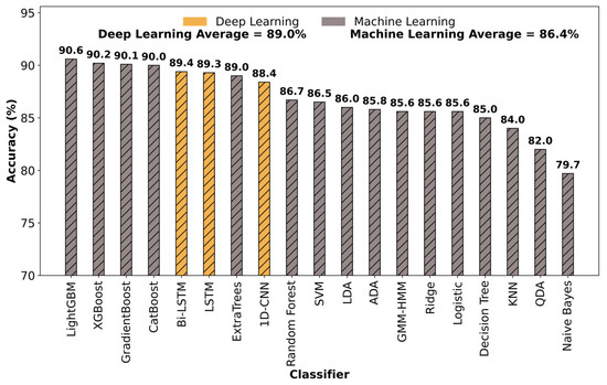
Figure 10.
Performance comparison between the average classification accuracies of deep learning and machine learning algorithms used for 1D sound-based classification.
The comparative analysis between machine learning and deep learning models for 1D and time-series classification provides some valuable insights. While deep neural networks are often considered more robust in classification tasks due to their built-in feature selection capabilities, the performance of deep learning models in this study was slightly lower, compared to that of ensemble classifiers, such as LightGBM and CatBoost. These findings align with some previous studies where ensemble methods demonstrated superior performance over certain deep neural networks in sound classification [93]. One potential factor influencing this outcome may be the dataset size. Deep learning models generally require large datasets for effective training. Although the smallest window size of 0.046 s provided sufficient data points for training, the larger window sizes may have contained inadequate data points to robustly train the neural networks [94,95]. This is reflected in the significant drop in accuracy for all three deep learning models when using the largest window size of 0.743 seconds. In contrast, some previous studies indicate that ensemble and tree-based algorithms, such as CatBoost and LightGBM, incorporate built-in regularization and boosting mechanisms, enabling them to perform well even with smaller datasets [96]. This trend is evident in the consistency of ensemble models across different window sizes, showing only minor changes in accuracy. For instance, the LightGBM classifier exhibited a slight accuracy change from 90.1% to 90.7% between the 0.372- and 0.743-second windows, whereas the Bi-LSTM model experienced a more substantial decline in performance from 89.7% to 86.3%, representing a 3.4% drop compared to the 0.6% change observed in LightGBM. The ability of gradient-boosting algorithms to maintain stable performance despite smaller dataset sizes may have contributed to their advantage over deep learning models.
5.2. Comparison Between Custom-Trained Deep Learning Models and Pre-Trained Neural Networks
Figure 11 shows a performance comparison between the custom-trained and pre-trained models using the three different types of image features: (a) time-series images, (b) spectrogram images, and (c) MFCC images. The figure shows three key findings. First, the hybrid CNN-LSTM model achieved the highest accuracy across all feature categories, outperforming all pre-trained models. Specifically, it attained the highest accuracy of 94.9% when MFCC features were used and performed better than the DenseNet169 model, which was the best-performing pre-trained model across all feature categories. Second, three of the pre-trained models—InceptionV3, InceptionResNetV2, and DenseNet169—outperformed the traditional CNN model. However, when spectrogram and MFCC features were used, the traditional CNN outperformed the pre-trained ResNet50 model. Third, while the CNN-LSTM model achieved its highest accuracy with MFCC features, the traditional CNN, along with InceptionV3, InceptionResNetV2, and DenseNet169, exhibited its best performance when spectrogram images were utilized.
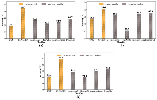
Figure 11.
Performance comparison between custom-trained and pre-trained models using three image features (a) time-series images; (b) spectrogram images; (c) MFCC.
These comparative findings provide some important insights. The CNN-LSTM model outperformed both the pre-trained networks and the traditional CNN. While pre-trained models such as InceptionV3, DenseNet169, and ResNet50 have been extensively trained on diverse image datasets and incorporate enhancements to improve performance, they remain fundamentally CNN-based architectures. In contrast, the hybrid CNN-LSTM network integrates the strengths of both CNNs and LSTMs, offering a distinct advantage. CNNs excel in capturing spatial features and hierarchical feature learning, while LSTMs are particularly effective at recognizing temporal patterns and dependencies within datasets [97]. By combining these two architectures, the hybrid model leverages both spatial and temporal feature extraction and feature learning techniques, leading to superior classification performance. This aligns with previous studies that have demonstrated the effectiveness of hybrid models in various classification tasks compared to traditional models such as CNN [98].
6. Conclusions
This study investigated the feasibility of combining audio signals with machine and deep learning algorithms to detect near-miss events such as slips and trips. To achieve this, the unique sound patterns associated with slip and trip events were recorded using a smartwatch. Then, 1D and 2D image features were extracted from the preprocessed audio signals and used to train several machine learning and deep learning models. This study provided some key insights. First, the hybrid CNN-LSTM model was the best-performing algorithm in slip and trip detection, achieving the highest accuracy of 0.966 when MFCC image features were used. Second, 2D feature-based models outperformed the 1D feature-based models. The best classifier when 1D features were used was the LightGBM model, achieving an average accuracy of 0.906 across the five windows considered. On the other hand, the hybrid CNN-LSTM model achieved an average accuracy of 0.949 across the five windows when MFCC features were used. Third, 1D MFCC features achieved an accuracy of 0.867, outperforming other feature categories such as time-domain features and frequency domain, which had average accuracies of 0.795 and 0.779, respectively.
In comparison to studies that have presented various methods for the detection of near-miss events, such as slips and trips, this study presents some new knowledge and academic findings. First, this study highlights the potential of using audio signals combined with machine and deep learning algorithms to detect slips and trips of construction workers. This presents a complementary method that addresses the limitations of manual monitoring, physical assessment techniques, and vision-based methods. Second, this study compares the performance of various 1D features and that of 2D features in slip and trip classification, therefore revealing the robustness of various image and time-series sound features in detecting unsafe events. Finally, this study, by testing various traditional, hybrid, and pre-trained models, provides a comprehensive understanding of the performance of various algorithms in sound classification, serving as a reference for future studies.
Practically, the findings of this study provide significant contributions to improving construction safety. This study introduces a novel sound-based classification approach for detecting unsafe events and near-miss occurrences such as slips and trips. While vision-based methods and physical response techniques, such as gait assessment, have been used, this study presents a complementary method to address the limitations, such as occlusion challenges with vision-based methods and high misclassifications associated with physical response methods due to the complex movement of workers arising from construction tasks. The sound-based method presented in this study overcomes these limitations and presents a more lightweight and less complex alternative for detecting slips and trips of construction workers. By utilizing this approach, sound-based algorithms can be developed and attached to various safety equipment, as well as other wearable sensors, for continuous monitoring to identify unsafe events such as slips and trips. From a management perspective, this study offers a proactive approach to identifying workers who are consistently vulnerable to slip and trip incidents. This enables targeted behavioral training, automatic documentation of near-miss events for safety management, and the identification of hazardous zones on construction sites where such incidents frequently occur. Ultimately, this approach has the potential to significantly enhance worker safety on construction sites. On a standard desktop computer (Intel Core i7 11700 CPU, 16 GB RAM, Windows 10, MATLAB/Python implementation), the feature extraction and classification for each event can be completed within a few hundred milliseconds, which is sufficient to support near-real-time analysis. Therefore, the proposed approach has the potential to be further optimized and integrated into an online framework capable of automatically issuing alarms when unsafe events are detected. In addition, the proposed approach shows strong potential for real-time on-site deployment. With integration into wearable devices such as smart helmets, smartwatches, or safety vests, the sound-based classification model can continuously capture ambient audio and process it locally or through edge-computing units. This enables instantaneous detection of slips and trips directly on the construction site, triggering real-time alerts to both the worker and the safety management team. Such a deployment strategy, relying on lightweight and low-power hardware, allows seamless operation without interfering with normal construction tasks. By combining this capability with existing monitoring systems, the proposed approach can effectively close the loop between detection and timely intervention, transforming safety management from a reactive process into a proactive and dynamic real-time protection system.
Although several important insights are presented in this study, it is crucial to highlight some limitations that may have influenced this study and present some directions for future research. First, the slip and trip sounds in this study were recorded in controlled environments, which may deviate slightly from actual construction environments and may not fully replicate the biomechanical, impact, and acoustic characteristics of naturally occurring slips and trips. Although data augmentation was conducted and white noise was added to account for this noise, future studies should improve the findings’ generalizability by conducting actual on-site experiments with varying background sound conditions. Second, this study explored only two behaviors: slips and trips. Future studies should explore other near-miss occurrences to enhance the applicability of sound-based monitoring for construction worker safety. Third, the sample size also involved 10 subjects only, which might not fully capture all diverse sound features for effective generalization. Future studies should explore larger sample sizes and on-site experiments to provide more diverse features. Fourth, the data augmentation in this study was limited to some simple methods including the addition of white noise. Future studies should explore more complex augmentation methods such as the addition of real construction audio to account for the varying noise conditions on construction sites. The ratio of augmented to real datasets should also be studied to evaluate the impact of data augmentation methods on model performance. Fifth, the data labeling in this study was limited to three classes only, and windows were assigned a specific class if 50% of its duration corresponded with that event. As a feasibility study, this labeling was selected to maintain consistency and reduce complexity. Future studies should explore more nuanced labeling techniques by experimenting with higher threshold or probabilistic labeling to handle mixed-state windows, exploring multi-class labeling when windows overlap, and incorporating event-aligned windows to ensure the boundaries align more closely with event onset or offset times. Sixth, to further enhance the interpretability of the proposed CNN–LSTM model, future research will investigate the use of explainable AI techniques, such as saliency maps and Grad-CAM. These visualization tools can highlight the regions of the audio spectrogram that contribute most to the model’s classification of slips and trips, thereby offering valuable insights into the acoustic patterns associated with unsafe events, supporting both model validation and practical deployment and providing guidance for further optimization of deep learning model parameters. Seventh, this study aims to verify the feasibility of the proposed method in a controlled experimental setup, where uncertainties that may cause sound variability were kept as consistent. Data collection is necessary to extend to real construction sites with more diverse conditions, including variations in sensor position and orientation, the physical and behavioral characteristics of workers, the material of the workshop floor and footwear, and different movement patterns, to improve the robustness of the approach under such variability. Eighth, microphones and audio sensors can also be affected by humidity and ambient conditions; however, such influences typically manifest as signal-to-noise ratio degradation rather than persistent bias shifts. These impairments can often be mitigated through robust filtering, adaptive noise reduction, and model training under diverse environmental conditions. Future studies will focus on systematically evaluating these environmental sound effects on audio signals and developing advanced compensation techniques to ensure reliable slip and trip detection performance in real-world construction sites. Finally, future research could combine sound-based slip and trip monitoring techniques with GPS and location-tracking technologies. This will help detect slip and trip events while also providing insights into hazardous areas on site where these events occur.
Author Contributions
Conceptualization: F.L., F.X.D., M.-K.K., J.T., J.S. and D.-E.L.; methodology: F.X.D., J.T. and F.X.D.; software: F.L., J.T. and F.X.D.; validation: F.L., F.X.D. and J.T.; formal analysis: F.L., F.X.D. and J.T.; investigation: F.L., F.X.D. and M.-K.K.; resources: F.L., F.X.D. and J.T.; data curation: F.L., F.X.D., M.-K.K., J.T., J.S. and D.-E.L.; writing—original draft: F.L., F.X.D., M.-K.K., J.T., J.S. and D.-E.L.; writing—review and editing, F.L., F.X.D., M.-K.K., J.T., J.S. and D.-E.L.; visualization: F.L., F.X.D. and J.T.; supervision, M.-K.K. and D.-E.L.; funding acquisition: F.L., M.-K.K. and D.-E.L. All authors have read and agreed to the published version of the manuscript.
Funding
This research was supported by four funding sources: (1) the National Research Foundation of Korea (NRF) grant funded by the Korean Government (MSIP) (No. 2018R1A5A1025137), (2) the National Research Foundation of Korea (NRF) grant funded by the Korea Government (MSIP) (No. 2021R1G1A1095119), (3) the National Natural Science Foundation of China (Grant No. 52308311) and (4) Natural Science Foundation of Jiangsu Provincial, China (Grant No. BK20230968).
Data Availability Statement
All data used during the study are available in a repository online through the link: https://github.com/lifangxin1007/sound-based- (accessed on 15 July 2025).
Conflicts of Interest
The authors declare no conflicts of interest.
Appendix A. Selected Hyperparameters for Various Classifiers
| Classifier | Selected Hyperparameters |
| Category and Boosting (CatBoost) | {‘eval_metric’: ‘Logloss’, ‘subsample’: 0.6, ‘depth’: 8, ‘learning_rate’: 0.1, ‘leaf_estimation_iterations’: 20, ‘bootstrap_type’: ‘MVS’, ‘max_leaves’: 64} |
| Light Gradient Boosting Machine (LightGBM) | {‘boosting_type’: ‘gbdt’, ‘colsample_bytree’: 0.5, ‘learning_rate’: 0.1, ‘min_child_samples’: 20, ‘min_child_weight’: 0.001, ‘n_estimators’: 150, ‘num_leaves’: 40, ‘max_depth’: 13} |
| Gradient Boosting Classifier (GBC) | {‘ccp_alpha’: 0.0, ‘criterion’: ‘friedman_mse’, ‘learning_rate’: 0.1, ‘loss’: ‘deviance’, ‘max_depth’: 10, ‘min_samples_leaf’: 2, ‘min_samples_split’: 4, ‘n_estimators’: 100, ‘subsample’: 1.0, ‘tol’: 0.0001} |
| Random Forest (RF) | {‘bootstrap’: True, ‘ccp_alpha’: 0.0, ‘criterion’: ‘gini’, ‘min_samples_leaf’: 1, ‘min_samples_split’: 2, ‘n_estimators’: 250, ‘max_features’: ‘sqrt’} |
| Extreme Gradient Boosting (XGBoost) | {‘objective’: ‘binary:logistic’, ‘base_score’: 0.5, ‘booster’: ‘gbtree’, ‘colsample_bylevel’: 1, ‘colsample_bynode’: 1, ‘colsample_bytree’: 1, ‘gamma’: 0, ‘learning_rate’: 0.1, ‘max_depth’: 7, ‘min_child_weight’: 1, ‘n_estimators’: 120, ‘num_parallel_tree’: 1, ‘reg_alpha’: 0, ‘reg_lambda’: 1, ‘scale_pos_weight’: 1} |
| Extra Trees (ET) | {‘bootstrap’: False, ‘ccp_alpha’: 0.0, ‘criterion’: ‘gini’, ‘max_features’: ‘sqrt’, ‘min_samples_leaf’: 5, ‘min_samples_split’: 2, ‘n_estimators’: 100} |
| Decision Tree (DT) | {‘criterion’: ‘gini’, ‘max_depth’: 14, ‘min_samples_leaf’: 7, ‘min_samples_split’: 2} |
| Quadratic Discriminant Analysis (QDA) | {‘priors’: None, ‘reg_param’: 0.0001, ‘tol’: 0.0001} |
| Adaptive Boosting (AdaBoost) | {‘algorithm’: ‘SAMME.R’, ‘n_estimators’: 350, ‘learning_rate’: 0.78} |
| Ridge Classifier (Ridge) | {‘alpha’: 2.0, ‘copy_X’: True, ‘fit_intercept’: True, ‘solver’: ‘auto’, ‘tol’: 0.001} |
| Linear Discriminant Analysis (LDA) | {‘solver’: ‘eigen’, ‘shrinkage’: ‘auto’, ‘n_components’: 1} |
| Logistic Regression (LR) | {‘C’: 1.5, ‘penalty’: ‘l2’, ‘solver’: ‘lbfgs’, ‘tol’: 0.0002, ‘class_weight’: ‘balanced’} |
| k-Nearest Neighbor (kNN) | {‘leaf_size’: 50, ‘metric’: ‘manhattan’, ‘n_neighbors’: 3} |
| Support Vector Machine (SVM)—Polynomial | {‘tol’: 0.0001, ‘max_iter’: 2000, ‘gamma’: ‘scale’, ‘C’: 1000.0} |
| Naïve Bayes | {‘priors’: None, ‘var_smoothing’: 1 × 10⁻⁹} |
| Bidirectional-LSTM (Bi-LSTM) | {‘dropout_rate’: 0.30970, ‘learning_rate’: 0.002938, ‘batch_size’: 32, ‘epochs’: 35} |
| Long Short-Term Memory (LSTM) | {‘dropout_rate’: 0.34889, ‘learning_rate’: 0.002844, ‘batch_size’: 32, ‘epochs’: 43} |
| One-dimensional Convolutional Neural Network (1D-CNN) | {‘filters’: 48, ‘kernel_size’: 3, ‘dropout_rate’: 0.17919, ‘learning_rate’: 0.001974, ‘batch_size’: 32, ‘epochs’: 47} |
References
- Halabi, Y.; Xu, H.; Long, D.; Chen, Y.; Yu, Z.; Alhaek, F.; Alhaddad, W. Causal factors and risk assessment of fall accidents in the US construction industry: A comprehensive data analysis (2000–2020). Saf. Sci. 2022, 146, 105537. [Google Scholar] [CrossRef]
- Lipscomb, H.J.; Glazner, J.E.; Bondy, J.; Guarini, K.; Lezotte, D. Injuries from slips and trips in construction. Appl. Ergon. 2006, 37, 267–274. [Google Scholar] [CrossRef]
- Antwi-Afari, M.F.; Li, H.; Seo, J.; Wong, A.Y.L. Automated detection and classification of construction workers’ loss of balance events using wearable insole pressure sensors. Autom. Constr. 2018, 96, 189–199. [Google Scholar] [CrossRef]
- Yang, K.; Ahn, C.R.; Vuran, M.C.; Aria, S.S. Semi-supervised near-miss fall detection for ironworkers with a wearable inertial measurement unit. Autom. Constr. 2016, 68, 194–202. [Google Scholar] [CrossRef]
- Aulin, R.; Linderbäck, E. Near-miss reporting among construction workers. In Proceedings of the CIB W099 International Conference on Achieving Sustainable Construction Health and Safety, Lund, Sweden, 2–3 June 2014; Lund University, Sweden Ingvar Kamprad Design Centre (IKDC): Lund, Sweden, 2014; p. 430. [Google Scholar]
- McKinnon, R.C. Safety Management: Near Miss Identification, Recognition, and Investigation; CRC Press: Boca Raton, FL, USA, 2012; ISBN 1439879478. [Google Scholar]
- Woźniak, Z.; Hoła, B. Analysing near-miss incidents in construction: A systematic literature review. Appl. Sci. 2024, 14, 7260. [Google Scholar] [CrossRef]
- Howcroft, J.; Kofman, J.; Lemaire, E.D. Review of fall risk assessment in geriatric populations using inertial sensors. J. Neuroeng. Rehabil. 2013, 10, 91. [Google Scholar] [CrossRef] [PubMed]
- Misnan, M.S.; Mustapa, M.; Ramly, Z.M.; Mohamed, S.F.; Rahim, F.N.A. Best practice of reporting accident and safety culture in construction site. Plan. Malays. 2024, 22, 90–103. [Google Scholar] [CrossRef]
- Haas, E.J.; Demich, B.; McGuire, J. Learning from Workers’ Near-miss Reports to Improve Organizational Management. Min. Metall. Explor. 2020, 37, 873–885. [Google Scholar] [CrossRef]
- Jebelli, H.; Ahn, C.R.; Stentz, T.L. Fall risk analysis of construction workers using inertial measurement units: Validating the usefulness of the postural stability metrics in construction. Saf. Sci. 2016, 84, 161–170. [Google Scholar] [CrossRef]
- Lee, S.; Koo, B.; Yang, S.; Kim, J.; Nam, Y.; Kim, Y. Fall-from-height detection using deep learning based on IMU sensor data for accident prevention at construction sites. Sensors 2022, 22, 6107. [Google Scholar] [CrossRef]
- Moohialdin, A.; Lamari, F.; Marc, M.; Trigunarsyah, B. A real-time computer vision system for workers’ PPE and posture detection in actual construction site environment. In Proceedings of the EASEC16: 16th East Asian-Pacific Conference on Structural Engineering and Construction, Brisbane, Australia, 3–6 December 2019; pp. 2169–2181. [Google Scholar]
- Fang, W.; Ding, L.; Luo, H.; Love, P.E.D. Falls from heights: A computer vision-based approach for safety harness detection. Autom. Constr. 2018, 91, 53–61. [Google Scholar] [CrossRef]
- Mushtaq, Z.; Su, S. Environmental sound classification using a regularized deep convolutional neural network with data augmentation. Appl. Acoust. 2020, 167, 107389. [Google Scholar] [CrossRef]
- Han, S.; Lee, S. A vision-based motion capture and recognition framework for behavior-based safety management. Autom. Constr. 2013, 35, 131–141. [Google Scholar] [CrossRef]
- Sabillon, C.A.; Cheng, C.F.; Rashidi, A.; Davenport, M.A.; Anderson, D.V. Activity analysis of construction equipment using audio signals and support vector machines. Autom. Constr. 2017, 81, 240–253. [Google Scholar] [CrossRef]
- Sherafat, B.; Rashidi, A.; Asgari, S. Sound-based multiple-equipment activity recognition using convolutional neural networks. Autom. Constr. 2022, 135, 104104. [Google Scholar] [CrossRef]
- Palmerini, L.; Klenk, J.; Becker, C.; Chiari, L. Accelerometer-based fall detection using machine learning: Training and testing on real-world falls. Sensors 2020, 20, 6479. [Google Scholar] [CrossRef] [PubMed]
- Yang, K.; Ahn, C.R.; Vuran, M.C.; Kim, H. Collective sensing of workers’ gait patterns to identify fall hazards in construction. Autom. Constr. 2017, 82, 166–178. [Google Scholar] [CrossRef]
- Kuhar, P.; Sharma, K.; Hooda, Y.; Verma, N.K. Internet of Things (IoT) based Smart Helmet for Construction. J. Phys. Conf. Ser. 2021, 1950, 12075. [Google Scholar] [CrossRef]
- Rajendran, S.; Giridhar, S.; Chaudhari, S.; Gupta, P.K. Technological advancements in occupational health and safety. Meas. Sens. 2021, 15, 100045. [Google Scholar] [CrossRef]
- Rasouli, S.; Alipouri, Y.; Chamanzad, S. Smart Personal Protective Equipment (PPE) for construction safety: A literature review. Saf. Sci. 2024, 170, 106368. [Google Scholar] [CrossRef]
- Homayounfar, S.Z.; Andrew, T.L. Wearable Sensors for Monitoring Human Motion: A Review on Mechanisms, Materials, and Challenges. SLAS Technol. 2020, 25, 9–24. [Google Scholar] [CrossRef]
- Gietzelt, M.; Nemitz, G.; Wolf, K.; Meyer Zu Schwabedissen, H.; Haux, R.; Marschollek, M. A clinical study to assess fall risk using a single waist accelerometer. Inform. Health Social Care 2009, 34, 181–188. [Google Scholar] [CrossRef] [PubMed]
- Ramachandran, A.; Karuppiah, A. A Survey on Recent Advances in Wearable Fall Detection Systems. BioMed Res. Int. 2020, 2020, 2167160. [Google Scholar] [CrossRef]
- Torres-Guzman, R.A.; Paulson, M.R.; Avila, F.R.; Maita, K.; Garcia, J.P.; Forte, A.J.; Maniaci, M.J. Smartphones and Threshold-Based Monitoring Methods Effectively Detect Falls Remotely: A Systematic Review. Sensors 2023, 23, 1323. [Google Scholar] [CrossRef]
- Fang, Y.C.; Dzeng, R.J. Accelerometer-based fall-portent detection algorithm for construction tiling operation. Autom. Constr. 2017, 84, 214–230. [Google Scholar] [CrossRef]
- Guo, Y.; Zhang, Z.; Chang, L.; Yu, J.; Ren, Y.; Chen, K.; Cao, H.; Xie, H. Temperature compensation for MEMS accelerometer based on a fusion algorithm. Micromachines 2024, 15, 835. [Google Scholar] [CrossRef]
- Lee, H.; Sohn, J.; Lee, G.; Jacobs, J.V.; Lee, S. A Graph-Based approach for individual fall risk assessment through a wearable inertial measurement unit sensor. Adv. Eng. Inform. 2025, 66, 103413. [Google Scholar] [CrossRef]
- Yuhai, O.; Kim, H.; Choi, A.; Mun, J.H. Deep learning-based slip-trip falls and near-falls prediction model using a single inertial measurement unit sensor for construction workplace. In Proceedings of the 2023 4th International Conference on Big Data Analytics and Practices (IBDAP), Bangkok, Thailand, 25–27 August 2023; pp. 1–6. [Google Scholar]
- Park, S.; Youm, M.; Kim, J. IMU Sensor-Based Worker Behavior Recognition and Construction of a Cyber—Physical System Environment. Sensors 2025, 25, 442. [Google Scholar] [CrossRef] [PubMed]
- Kim, H.; Ahn, C.R.; Stentz, T.L.; Jebelli, H. Assessing the effects of slippery steel beam coatings to ironworkers’ gait stability. Appl. Ergon. 2018, 68, 72–79. [Google Scholar] [CrossRef] [PubMed]
- Khan, M.; Nnaji, C.; Khan, M.S.; Ibrahim, A.; Lee, D.; Park, C. Risk factors and emerging technologies for preventing falls from heights at construction sites. Autom. Constr. 2023, 153, 104955. [Google Scholar] [CrossRef]
- Paneru, S.; Jeelani, I. Computer vision applications in construction: Current state, opportunities & amp; challenges. Autom. Constr. 2021, 132, 103940. [Google Scholar] [CrossRef]
- Han, S.; Lee, S.; Peña-Mora, F. Vision-based motion detection for safety behavior analysis in construction. In Proceedings of the Construction Research Congress 2012: Construction Challenges in a Flat World, West Lafayette, IN, USA, 21–23 May 2012; pp. 1032–1041. [Google Scholar]
- Han, S.; Lee, S.; Peña-Mora, F. Comparative Study of Motion Features for Similarity-Based Modeling and Classification of Unsafe Actions in Construction. J. Comput. Civil. Eng. 2014, 28, A4014005. [Google Scholar] [CrossRef]
- Fang, Q.; Li, H.; Luo, X.; Ding, L.; Luo, H.; Li, C. Computer vision aided inspection on falling prevention measures for steeplejacks in an aerial environment. Autom. Constr. 2018, 93, 148–164. [Google Scholar] [CrossRef]
- Ding, L.; Fang, W.; Luo, H.; Love, P.E.D.; Zhong, B.; Ouyang, X. A deep hybrid learning model to detect unsafe behavior: Integrating convolution neural networks and long short-term memory. Autom. Constr. 2018, 86, 118–124. [Google Scholar] [CrossRef]
- Lee, H.; Jeon, J.; Lee, D.; Park, C.; Kim, J.; Lee, D. Game engine-driven synthetic data generation for computer vision-based safety monitoring of construction workers. Autom. Constr. 2023, 155, 105060. [Google Scholar] [CrossRef]
- Bonyani, M.; Soleymani, M.; Wang, C. Construction workers’ unsafe behavior detection through adaptive spatiotemporal sampling and optimized attention based video monitoring. Autom. Constr. 2024, 165, 105508. [Google Scholar] [CrossRef]
- Lee, Y.; Scarpiniti, M.; Uncini, A. Advanced Sound Classifiers and Performance Analyses for Accurate Audio-Based Construction Project Monitoring. J. Comput. Civil. Eng. 2020, 34, 04020030. [Google Scholar] [CrossRef]
- Sabillon, C.A.; Rashidi, A.; Samanta, B.; Cheng, C.; Davenport, M.A.; Anderson, D.V. A productivity forecasting system for construction cyclic operations using audio signals and a Bayesian approach. In Proceedings of the Construction Research Congress 2018, New Orleans, LA, USA, 2–4 April 2018; pp. 295–304. [Google Scholar]
- Liu, Z.; Li, S. A sound monitoring system for prevention of underground pipeline damage caused by construction. Autom. Constr. 2020, 113, 103125. [Google Scholar] [CrossRef]
- Rashid, K.M.; Louis, J. Activity identification in modular construction using audio signals and machine learning. Autom. Constr. 2020, 119, 103361. [Google Scholar] [CrossRef]
- Mannem, K.R.; Mengiste, E.; Hasan, S.; de Soto, B.G.; Sacks, R. Smart audio signal classification for tracking of construction tasks. Autom. Constr. 2024, 165, 105485. [Google Scholar] [CrossRef]
- Collado-Villaverde, A.; R-Moreno, M.D.; Barrero, D.F.; Rodriguez, D. Machine Learning Approach to Detect Falls on Elderly People Using Sound. In Proceedings of the International Conference on Industrial, Engineering and Other Applications of Applied Intelligent Systems, Arras, France, 27–30 June 2017. [Google Scholar]
- Kaur, P.; Wang, Q.; Shi, W. Fall detection from audios with Audio Transformers. Smart Health 2022, 26, 100340. [Google Scholar] [CrossRef]
- Garcia, A.; Huang, X. SAFE: Sound Analysis for Fall Event detection using machine learning. Smart Health 2025, 35, 100539. [Google Scholar] [CrossRef]
- Zhang, T.; Lee, Y.; Scarpiniti, M.; Uncini, A. A supervised machine learning-based sound identification for construction activity monitoring and performance evaluation. In Proceedings of the Construction Research Congress 2018, New Orleans, LA, USA, 2–4 April 2018; pp. 358–366. [Google Scholar]
- McLoughlin, I.; Xie, Z.; Song, Y.; Phan, H.; Palaniappan, R. Time–Frequency Feature Fusion for Noise Robust Audio Event Classification. Circuits Syst. Signal Process. 2020, 39, 1672–1687. [Google Scholar] [CrossRef]
- Pohlman, K. Principles of Digital Audio, 6th ed.; Digital Video/Audio; McGraw-Hill Professional: New York, NY, USA, 2010; ISBN 9780071663465. [Google Scholar]
- Nyquist, H. Certain Topics in Telegraph Transmission Theory. Trans. Am. Inst. Electr. Eng. 1928, 47, 617–644. [Google Scholar] [CrossRef]
- Watkinson, J. The Art of Digital Audio; Focal Press: Waltham, MA, USA, 2000; ISBN 0240515870. [Google Scholar]
- Stone, B. Perceptual Evaluation of Digital Audio Parameters in Psychoacoustic Research. Master’s Thesis, James Madison University, Harrisonburg, VA, USA, 2023; p. 8. [Google Scholar]
- Khorami, F.; Obaid, N.; Bhatnagar, T.; Ayoub, A.; Robinovitch, S.N.; Sparrey, C.J. Impact forces in backward falls: Subject-specific video-based rigid body simulation of backward falls. Proc. Inst. Mech. Eng. Part H J. Eng. Med. 2023, 237, 1275–1286. [Google Scholar] [CrossRef]
- Salamon, J.; Bello, J.P. Deep convolutional neural networks and data augmentation for environmental sound classification. IEEE Signal Process. Lett. 2017, 24, 279–283. [Google Scholar] [CrossRef]
- Ko, T.; Peddinti, V.; Povey, D.; Khudanpur, S. Audio augmentation for speech recognition. In Proceedings of the Interspeech, Dresden, Germany, 6–10 September 2015; p. 3586. [Google Scholar]
- Williams, Z.J.; He, J.L.; Cascio, C.J.; Woynaroski, T.G. A review of decreased sound tolerance in autism: Definitions, phenomenology, and potential mechanisms. Neurosci. Biobehav. Rev. 2021, 121, 1–17. [Google Scholar] [CrossRef] [PubMed]
- Zhang, Z.; Schuller, B. Semi-supervised learning helps in sound event classification. In Proceedings of the 2012 IEEE International Conference on Acoustics, Speech and Signal Processing (ICASSP), Kyoto, Japan, 25–30 March 2012; pp. 333–336. [Google Scholar]
- Shi, J.; Chang, X.; Guo, P.; Watanabe, S.; Fujita, Y.; Xu, J.; Xu, B.; Xie, L. Sequence to Multi-Sequence Learning via Conditional Chain Mapping for Mixture Signals. arXiv 2020, arXiv:2006.14150. [Google Scholar] [CrossRef]
- Venkatesh, S.; Moffat, D.; Miranda, E.R. You Only Hear Once: A YOLO-like Algorithm for Audio Segmentation and Sound Event Detection. Appl. Sci. 2022, 12, 3293. [Google Scholar] [CrossRef]
- Akhavian, R.; Behzadan, A.H. Smartphone-based construction workers’ activity recognition and classification. Autom. Constr. 2016, 71, 198–209. [Google Scholar] [CrossRef]
- Landeira, V.A.R.; Santos, J.O.; Nagano, H. Comparing and Combining Audio Processing and Deep Learning Features for Classification of Heartbeat Sounds. In Proceedings of the ICASSP 2024–2024 IEEE International Conference on Acoustics, Speech and Signal Processing (ICASSP), Seoul, Republic of Korea, 14–19 April 2024; pp. 7220–7224. [Google Scholar]
- Okaba, M.; Tuncer, T. An automated location detection method in multi-storey buildings using environmental sound classification based on a new center symmetric nonlinear pattern: CS-LBlock-Pat. Autom. Constr. 2021, 125, 103645. [Google Scholar] [CrossRef]
- Deng, M.; Meng, T.; Cao, J.; Wang, S.; Zhang, J.; Fan, H. Heart sound classification based on improved MFCC features and convolutional recurrent neural networks. Neural Netw. 2020, 130, 22–32. [Google Scholar] [CrossRef] [PubMed]
- Sangeetha, J.; Hariprasad, R.; Subhiksha, S. Analysis of machine learning algorithms for audio event classification using Mel-frequency cepstral coefficients. In Applied Speech Processing; Elsevier: Amsterdam, The Netherlands, 2021. [Google Scholar]
- Küçükbay, S.E.; Sert, M. Audio-based event detection in office live environments using optimized MFCC-SVM approach. In Proceedings of the 2015 IEEE 9th International Conference on Semantic Computing (IEEE ICSC 2015), Anaheim, CA, USA, 7–9 February 2015; pp. 475–480. [Google Scholar]
- He, X.; Zhao, K.; Chu, X. AutoML: A survey of the state-of-the-art. Knowl. Based Syst. 2021, 212, 106622. [Google Scholar] [CrossRef]
- Jurafsky, D.; Martin, J.H. Speech and Language Processing: International Edition, 2nd ed.; Pearson: Upper Saddle River, NJ, USA, 2008; ISBN 0135041961. [Google Scholar]
- Rabiner, L.R. A tutorial on hidden Markov models and selected applications in speech recognition. Proc. IEEE 1989, 77, 257–286. [Google Scholar] [CrossRef]
- Levy, J.; Naitsat, A.; Zeevi, Y.Y. Classification of audio signals using spectrogram surfaces and extrinsic distortion measures. Eurasip J. Adv. Signal Process. 2022, 2022, 100. [Google Scholar] [CrossRef]
- Wolf-Monheim, F. Spectral and Rhythm Features for Audio Classification with Deep Convolutional Neural Networks. arXiv 2024, arXiv:2410.06927. [Google Scholar] [CrossRef]
- Hochreiter, S.; Schmidhuber, J. Long Short-Term Memory. Neural Comput. 1997, 9, 1735–1780. [Google Scholar] [CrossRef] [PubMed]
- Shi, X.; Chen, Z.; Wang, H.; Yeung, D.; Wong, W.; Woo, W. Convolutional LSTM Network: A Machine Learning Approach for Precipitation Nowcasting. Adv. Neural Inf. Process. Syst. 2015, 28, 1–9. [Google Scholar]
- Karim, F.; Majumdar, S.; Darabi, H.; Harford, S. Multivariate LSTM-FCNs for time series classification. Neural Netw. 2019, 116, 237–245. [Google Scholar] [CrossRef]
- Gong, Y.; Chung, Y.; Glass, J. Ast: Audio spectrogram transformer. arXiv 2021, arXiv:2104.01778. [Google Scholar] [CrossRef]
- Bishop, C.M.; Nasrabadi, N.M. Pattern Recognition and Machine Learning; Springer: Berlin/Heidelberg, Germany, 2006. [Google Scholar]
- Piczak, K.J. Environmental sound classification with convolutional neural networks. In Proceedings of the 2015 IEEE 25th International Workshop on Machine Learning for Signal Processing (MLSP), Boston, MA, USA, 17–20 September 2015; pp. 1–6. [Google Scholar]
- Szegedy, C.; Ioffe, S.; Vanhoucke, V.; Alemi, A. Inception-v4, Inception-ResNet and the Impact of Residual Connections on Learning. In Proceedings of the AAAI Conference On Artificial Intelligence, Phoenix, AZ, USA, 12–17 February 2016. [Google Scholar]
- He, K.; Zhang, X.; Ren, S.; Sun, J. Deep Residual Learning for Image Recognition. arXiv 2015, arXiv:1512.03385. [Google Scholar] [CrossRef]
- Huang, G.; Liu, Z.; van der Maaten, L.; Weinberger, K.Q. Densely Connected Convolutional Networks. In Proceedings of the IEEE Conference on Computer Vision and Pattern Recognition, Las Vegas, NV, USA, 26 June–1 July 2016. [Google Scholar] [CrossRef]
- Aslam, M.A.; Zhang, L.; Liu, X.; Irfan, M.; Xu, Y.; Li, N.; Zhang, P.; Jiangbin, Z.; Yaan, L. Underwater sound classification using learning based methods: A review. Expert. Syst. Appl. 2024, 255, 124498. [Google Scholar] [CrossRef]
- Miao, Y.; Gowayyed, M.; Metze, F. EESEN: End-to-end speech recognition using deep RNN models and WFST-based decoding. In Proceedings of the 2015 IEEE workshop on automatic speech recognition and understanding (ASRU), Scottsdale, AZ, USA, 13–17 December 2015; pp. 167–174. [Google Scholar]
- Dahl, G.E.; Dong, Y.; Li, D.; Acero, A. Context-Dependent Pre-Trained Deep Neural Networks for Large-Vocabulary Speech Recognition. IEEE Trans. Audio Speech Lang. Process. 2012, 20, 30–42. [Google Scholar] [CrossRef]
- Islam, M.R.; Akhi, A.B.; Akter, F.; Rashid, M.W.; Rumu, A.I.; Lata, M.A.; Ashrafuzzaman, M. A Machine Learning Approach for Emotion Classification in Bengali Speech. Int. J. Adv. Comput. Sci. Appl. 2023, 14, 885–892. [Google Scholar] [CrossRef]
- Dorogush, A.V.; Ershov, V.; Gulin, A. CatBoost: Gradient boosting with categorical features support. arXiv 2018, arXiv:1810.11363. [Google Scholar] [CrossRef]
- Bhargavi, K.D.; Deepa, V.; Harshitha, I. Audio Classification through MFCC features using RNN algorithm. In Proceedings of the 2024 4th Asian Conference on Innovation in Technology (ASIANCON), Pimari Chinchwad, India, 23–25 August 2024; pp. 1–5. [Google Scholar]
- Mohammed, D.Y.; Al-Karawi, K.; Aljuboori, A. Robust speaker verification by combining MFCC and entrocy in noisy conditions. Bull. Electr. Eng. Inform. 2021, 10, 2310–2319. [Google Scholar] [CrossRef]
- Lebaka, L.N.; Govarthan, P.K.; Rani, P.; Ganapathy, N.; Agastinose Ronickom, J.F. Automated emotion recognition system using blood volume pulse and xgboost learning. In Healthcare Transformation with Informatics and Artificial Intelligence; IOS Press: Amsterdam, The Netherlands, 2023. [Google Scholar]
- Wibowo, R.; Soeleman, M.A.; Affandy, A. Hybrid Top-K Feature Selection to Improve High-Dimensional Data Classification Using Naïve Bayes Algorithm. Sci. J. Inform. 2023, 10, 113–120. [Google Scholar] [CrossRef]
- Constantinou, M.; Exarchos, T.; Vrahatis, A.G.; Vlamos, P. COVID-19 Classification on Chest X-ray Images Using Deep Learning Methods. Int. J. Environ. Res. Public Health 2023, 20, 2035. [Google Scholar] [CrossRef]
- Yerramreddy, D.R.; Marasani, J.; Gowtham, P.S.V.; Yashwanth, S.; SS, P. Speaker identification using MFCC feature extraction: A comparative study using GMM, CNN, RNN, KNN and random forest classifier. In Proceedings of the 2023 Second International Conference on Trends in Electrical, Electronics, and Computer Engineering (TEECCON), Bangalore, India, 23–24 August 2023; pp. 287–292. [Google Scholar]
- Yuan, H. Current perspective on artificial intelligence, machine learning and deep learning. Appl. Comput. Eng. 2023, 19, 116–122. [Google Scholar] [CrossRef]
- Ajakwe, S.O.; Deji-Oloruntoba, O.; Olatunbosun, S.O.; Duorinaah, F.X.; Bayode, I.A. Multidimensional Perspective to Data Preprocessing for Model Cognition Verity. In Recent Trends and Future Direction for Data Analytics; IGI Global Scientific Publishing: New York, NY, USA, 2024. [Google Scholar]
- Santoro, D.; Ciano, T.; Ferrara, M. A comparison between machine and deep learning models on high stationarity data. Sci. Rep. 2024, 14, 19409. [Google Scholar] [CrossRef]
- Goh, H.H.; He, B.; Liu, H.; Zhang, D.; Dai, W.; Kurniawan, T.A.; Goh, K.C. Multi-Convolution Feature Extraction and Recurrent Neural Network Dependent Model for Short-Term Load Forecasting. IEEE Access 2021, 9, 118528–118540. [Google Scholar] [CrossRef]
- Madhuri Ghuge, E.A. Deep Learning Driven QoS Anomaly Detection for Network Performance Optimization. J. Electr. Syst. 2024, 19, 97–104. [Google Scholar] [CrossRef]
Disclaimer/Publisher’s Note: The statements, opinions and data contained in all publications are solely those of the individual author(s) and contributor(s) and not of MDPI and/or the editor(s). MDPI and/or the editor(s) disclaim responsibility for any injury to people or property resulting from any ideas, methods, instructions or products referred to in the content. |
© 2025 by the authors. Licensee MDPI, Basel, Switzerland. This article is an open access article distributed under the terms and conditions of the Creative Commons Attribution (CC BY) license (https://creativecommons.org/licenses/by/4.0/).