Prediction of Skeleton Curves for Seismically Damaged RC Columns Based on a Data-Driven Machine-Learning Approach

Abstract

The skeleton curve plays a crucial role in evaluating the seismic capacity of damaged structures. The research explored the application of data-driven machine learning approaches to predict the skeleton curves of earthquake-damaged reinforced concrete (RC) columns. Various machine learning methods, including Lasso regression, K-nearest neighbor (KNN), support vector machine (SVM), decision tree, and AdaBoost, were employed to develop a machine learning prediction model (MLPM) for seismic-damaged RC columns. A substantial dataset for the MLPM was derived from finite element (FE) analysis results. The input parameters for the machine learning models included the design specifications of the numerical column model and the damage index (DI), while the coordinates of key points on the skeleton curves served as the output parameters. The findings indicated that the K-nearest neighbor algorithm exhibited the best predictive performance, particularly for the yielding and peak points. The most influential input feature for predicting peak strength was the shear span-to-effective depth ratio, followed by the DI. The ML-based models demonstrated higher efficiency than numerical simulations and theoretical calculations in predicting the skeleton curves of damaged RC columns.

1. Introduction

In recent years, many researchers have focused on applying machine learning methods to the field of civil engineering. Due to their excellent feature extraction and prediction capabilities, machine learning methods have been particularly successful in providing accurate results for complex regression models, leading to significant research achievements.

Machine learning methods have been widely adopted in structural engineering. For example, Naderpour and Mirrashid [1] employed artificial neural networks to predict the flexural capacity of reinforced concrete (RC) columns using test results from the PEER database. Similarly, Ning et al. [2] applied artificial intelligence techniques to predict the hysteresis curves of RC columns based on the test data of 251 RC columns. Luo and Paal [3] proposed the use of support vector machines to predict the lateral deformation capacity of RC columns.

Machine learning has also been successfully applied in earthquake engineering. Xie et al. [4] provided an overview of machine learning methods and introduced their application in seismic hazard analysis, structural damage identification, vulnerability assessment, and structural control. Asim et al. [5] employed four machine learning techniques, including pattern recognition neural networks, recurrent neural networks, random forests, and boost ensemble methods, to predict earthquake magnitudes. Xiong et al. [6] and Balz et al. [7] utilized machine learning algorithms with UAV and satellite images to identify post-earthquake damage and assess the extent of structural damage. Jiang et al. [8] developed an artificial neural network model to predict the dynamic response of bridges under seismic loading, while Pang et al. [9] applied neural networks to generate fragility curves for bridges using the Incremental Dynamic Analysis (IDA) method. Giovanis et al. [10] predicted the maximum displacement drift and fragility curves of frame buildings under varying earthquake intensities. Su et al. [11] used decision trees to predict damage to frame structures, and Kia et al. [12] employed support vector machines and artificial neural networks to predict the seismic response of frame structures. Furthermore, Morfidis et al. [13,14,15] conducted studies using artificial neural networks to predict displacement drift time histories for three-dimensional frame structures and present seismic analysis results based on these prediction models. Harirchian et al. [16] used post-earthquake damage databases to predict the damage states of RC buildings with artificial neural networks.

Several researchers have demonstrated the accuracy of machine learning methods in predicting the performance of damaged structures. Zhang et al. [17] proposed a machine learning framework to assess the post-earthquake safety of structures. Using sequential ground motions, they performed Incremental Dynamic Analysis to calculate the residual collapse capacity of structures and employed machine learning methods to rapidly identify the damage states of seismically damaged buildings. Mangalathu et al. [18] used various machine learning techniques, such as discriminant analysis, K-nearest neighbors, decision trees, and random forests, to identify the damage states of post-earthquake buildings. Their results showed that the random forest method achieved a high accuracy of 66% in predicting structural damage states. Notable progress has also been made in addressing uncertainty effects in damaged structural analysis. For instance, Palanci [19] used Monte Carlo simulation and supervised learning methods to handle uncertainties in seismic risk assessment of one-story precast industrial buildings, establishing important methodological foundations for damage-related predictions using fuzzy logic approaches.

Many scholars have also explored the use of machine learning to predict the seismic capacity of earthquake-damaged RC columns. Han et al. [20] employed a deep feed-forward neural network to establish relationships between the response parameters of seismically damaged structures and seven key parameters of RC structural models, including site type, earthquake intensity, number of structural layers, standard layer height, span in the X-direction, and spans in both X- and Y-directions. This study further developed a framework for assessing the regional earthquake damage of RC structures and quantifying the resulting building losses. In another study, Han et al. [21] used deep learning techniques to predict the lumped plastic hinge parameters of RC beams based on test data under cyclic loading. The model took characteristic member parameters as inputs and predicted coordinates of key points on the skeleton curve and hysteresis parameters as outputs. Compared to traditional nonlinear dynamic analysis and existing empirical formulations, the machine learning model demonstrated higher accuracy. Ludovico et al. [22] modified the moment-rotation plastic hinge model of damaged RC columns and proposed modification factors for strength, stiffness, and displacement based on rotation ductility demand. However, their model was based on experimental data rather than machine learning methods. Li et al. [23] developed a new damage distribution model along the height of the plastic hinge zone and proposed a model to evaluate the residual capacity of earthquake-damaged RC columns by modifying the material properties of the damaged concrete and reinforcement. Although effective, this study relied on test data and nonlinear dynamic analysis rather than machine learning, which limited the model’s scope and efficiency. Todorov and Billah [24] evaluated the seismic capacity of bridge columns using various machine learning methods based on numerical results from nonlinear time history analysis and pushover analysis for 20 column models. The efficient prediction of residual seismic capacity enabled rapid evaluation of retrofitting strategies for damaged RC columns. By accurately predicting damaged skeleton curves, the machine learning framework could help engineers quickly identify vulnerable columns, quantify performance deficits, and optimize retrofitting interventions [25,26].

These studies demonstrate the high efficiency and accuracy of machine learning methods in predicting seismic response and structural capacity. However, despite the progress achieved in past research, several critical research gaps remain in the research fields that limit the practical application of machine learning in post-earthquake structural assessment. While some studies have addressed damaged structures, most machine learning applications in structural engineering still focus predominantly on intact structures, with limited systematic investigation of earthquake-damaged structures across varying damage levels. Additionally, existing approaches lack a unified framework that can predict complete skeleton curves (covering elastic, yielding, peak, and post-peak phases) for damaged RC columns using damage index as comprehensive input parameters that encapsulate the cumulative effects of earthquake loading. Moreover, a limited number of columns and restricted output parameters in previous studies have hindered the development of machine learning models with broad adaptability, particularly those that can adjust and modify predictions based on varying levels of structural damage. Finally, most existing datasets are relatively small and cover limited parameter ranges, which constrain the generalization capability of trained models across diverse structural configurations and damage scenarios.

To address these research gaps comprehensively, this study focused on developing a robust machine learning framework for predicting the skeleton curves of earthquake-damaged RC columns at different damage levels. The research developed an extensive database comprising a large-scale set of simulations from multiple column models across all damage levels, providing a comprehensive data foundation for the machine learning model. A machine learning model was developed that predicted the skeleton curve of RC columns as a direct function of their pre-existing damage level, quantified by the damage index, enabling damage-informed prediction of residual structural performance. The approach could reconstruct entire damaged skeleton curves through multiple characteristic points using optimized machine learning algorithms, providing a comprehensive assessment of residual strength, stiffness, and ductility. This study conducted a systematic evaluation of seismic capacity degradation patterns and quantitative analysis using PCA and SHAP methods to identify key input parameters affecting post-earthquake performance, providing practical insights for evaluation and retrofitting.

The data for the machine learning models were derived from numerical analysis results using a unique “earthquake-then-cyclic-loading” simulation protocol. A distinctive loading mode, consisting of earthquake dynamic loading followed by cyclic loading, was applied to generate hysteresis curves for columns with varying levels of damage. The characteristic parameters of the column model and the damage index (DI) were used as input parameters, while the coordinates of characteristic points on the skeleton curves and degradation parameters were the output parameters. The predicted skeleton curves were compared to actual simulation results, and the importance of input parameters influencing the output was analyzed. The proposed model was also used to evaluate the degradation of seismic capacity in earthquake-damaged columns. This approach can be applied to assess the residual seismic capacity of damaged columns after a mainshock or quickly calculate the seismic response to aftershocks. It could play a crucial role in post-earthquake structural safety assessments, regional loss estimations, and the efficient selection of appropriate seismic retrofitting strategies.

2. Seismic Damaged RC Column Database

For machine learning methods, the establishment of a robust database is crucial. In this study, the data used for building machine learning models were obtained from a large number of simulation results derived from finite element (FE) analysis. A total of 1350 column models with varying parameters were created using the OpenSEES (v2.5.0) platform. Fifty ground motion records were selected. The peak ground acceleration (PGA) of each ground motion record was scaled to 0.1 g, 0.3 g, 0.5 g, 0.7 g, and 0.9 g. For each column experiencing different damage levels due to the earthquake, pseudo-static loading was applied following the dynamic earthquake loading. The skeleton curves of RC columns after pseudo-static loading, referred to as “damaged skeleton curves”, were extracted to form the numerical simulation dataset, which served as the sample database for the machine learning methods.

2.1. Characteristic Parameters of Columns

Extensive finite element analyses were conducted on various numerical models of RC columns. Five key parameters were varied within reasonable ranges for the models: aspect ratio (λ), longitudinal reinforcement ratio (ρ_l), concrete compressive strength (f_c), yield strength of the longitudinal reinforcement (f_yl), and the axial compression ratio (n). As a result, a wide variety of FE models were generated, representing RC columns with different sizes, steel reinforcement configurations, material strengths, and boundary conditions.

The values of each characteristic parameter were determined as follows: Considering that it was unrealistic to include all FE models of columns with all kinds of section sizes, reinforcements, and material strengths in the sample database in the investigation, the heights of all columns were set to 1.0 m. The columns were square in section. The section widths of columns were calculated according to the formula of aspect ratio. In terms of aspect ratios of columns, the values were set to 5, 4.5, 4, and 3.5, which was a common range for this variable. Three longitudinal reinforcement ratios of 0.75%, 1.15%, and 1.55% were selected to represent low reinforcement ratio, medium reinforcement ratio, and high reinforcement ratio, respectively, which satisfied the requirements in the Chinese seismic code [27]. The axial compressive strength of concrete corresponded to 20.1 MPa, 23.4 MPa, and 26.8 MPa, respectively, while the yield strength of longitudinal reinforcement was 400 MPa and 500 MPa, respectively. These are the most widely used material strengths. Five axial compression ratios ranging from 0.1 to 0.9 were chosen for ordinary frame buildings.

In total, 1350 column models were created in this study. For columns not included in the sample, linear interpolation can be used to determine the parameters. For columns with different heights or section sizes, the corresponding parameters can be scaled according to the ratio of the dimensions. In the research, section dimensions and steel bar diameters were not explicitly listed, nor were their values directly provided. Instead, parameters such as reinforcement ratio, aspect ratio, and axial compression ratio were used, making the models more general and widely applicable. The approach has also been recognized and adopted in the literature [28].

2.2. Ground Motion Parameters

The loading scheme for the columns in the numerical simulations is as follows: Initially, the RC column models were subjected to ground motions of various types and amplitudes, resulting in different levels of damage to the columns. These damaged RC columns were then subjected to a cyclic loading protocol, and the skeleton curves of the damaged columns were obtained. The ground motions induced varying degrees of seismic dynamic damage to the columns, while the cyclic loading protocol was used to evaluate the residual seismic capacity by extracting the damaged skeleton curves. The ground motion records utilized in this study were sourced from the PEER database (https://peer.berkeley.edu/research/databases, 25 August 2025). A total of 50 ground motion records were selected, as shown in

Table 1. Ground motion records in numerical analysis.

EQ	Station	Component	Number	EQ	Station	Component	Number
ChiChi	TCU071	N/E	10	Northridge	E-RRS	228/318	8
	TCU122	E			FAR	000/090
	TCU129	N			MU2	035/125
	CHY101	E			TUJ	262/352
	HWA032	N		Petrolia	CE89156	000/090	2
	HWA2	N/E		Umbria Marche	A-AAL	018/108	2
	CHY046	N/E		Chalfant Valley	A-LAD	180	1
Racha	Ambrolauri	X/Y	2	Whittier Narrows	A-ALT	000/090	9
Mt. Hengill Area	Hveragerdi	Y	1		A-CAM	009/279
Kefallinia island	Argostoli	X/Y	4		A-DEL	000/090
	Kefallinia	X/Y			A-MTW	000
South Iceland	Kaldarholt	Y	1		A-GRN	180
Duzce	LDEO	X/Y	2		A-SMA	270
Imperial Valley	A-E06	140/230	4	WenChuan	051LXS	NS	6
	A-E08	140/230			051LXT	EW/NS
Darfield	NZHVSC	S64E/S26W	3		051MZQ	NS
	NZLPCC	S10E			051WCW	EW/NS

. Each record was required to include necessary information, such as station details and directions. Each record should have the peak ground acceleration (PGA) greater than 0.1 g.

When selecting the ground motions, both significant duration (defined as the time interval over which a specified percentage of the total energy is accumulated) [29] and mean period (a preferred frequency content parameter that characterizes the frequency content of earthquake ground motion by averaging periods in the Fourier amplitude spectrum) [30,31] were thoroughly considered to ensure broad coverage of ground motion characteristics. These parameters are widely used for ground motion characterization, structural response analysis, and seismic hazard assessment. Most of the selected ground motions were from typical earthquakes recorded at various locations. The significant durations of the ground motions listed in Table 1 range from 0 to 75 s, while the mean periods range from 0 to 1.3 s, reflecting a wide distribution of ground motion characteristics.

To induce varying degrees of damage to the columns, the PGA of each ground motion was scaled from 0.1 g to 0.9 g in increments of 0.2 g, resulting in a total of five different amplitude levels. Consequently, the response results of the same column model under 250 groups of seismic loadings were obtained, covering a full range of damage levels, from minor to severe. The damage index (DI) for each column after these 250 seismic loadings was also calculated. The damage index (DI) is defined in the literature [28] as follows:

$$DI={\displaystyle \frac{{\theta }_m-{\theta }_y}{{\theta }_u-{\theta }_y}}+\beta {\displaystyle \frac{E_h}{M_y{\theta }_u}}$$

(1)

where θ_m is the maximum rotation; θ_y and θ_u are the yielding and ultimate rotations of structural members, respectively; E_h represents the hysteretic energy; M_y is the yielding moment of structural members; and β is the hysteretic energy factor, which was set to 0.15 as recommended for frame structures.

As a result, the damage index (DI) can range from nearly 0 to values exceeding 1, depending on the amplitude of ground motion, thus providing a comprehensive representation of all damage levels. In actual simulation results, different columns may exhibit the same DI under identical ground motions, or a single column may reach the same DI under varying ground motions. However, machine learning facilitates the identification of overall trends through big data analysis. Therefore, in addition to the characteristic parameters of the column models, the DI from seismic loadings is an essential input parameter for the machine learning models.

3. ML-Based Approach for Skeleton Curves of Seismically Damaged RC Columns

3.1. Input Parameters

In the machine learning model, six input parameters were selected to accurately account for the factors affecting the seismic performance of the columns. These parameters include five characteristic parameters of the column model and one damage index (DI) parameter, which were used to predict the skeleton curves of the seismic-damaged columns. The five characteristic parameters are aspect ratio (λ), longitudinal reinforcement ratio (ρ_l), concrete compressive strength (f_c), yield strength of the longitudinal reinforcement (f_yl), and the axial compression ratio (n). It is important to note that the damage index (DI) was used as an input parameter instead of direct ground motion parameters. The reason is that the calculation of the DI inherently incorporates the effects of ground motion on the model, thus providing a comprehensive and direct reflection of the damage sustained by the column.

Table 2. The value ranges and value selection methods of input parameters.

Categorization	Input Parameters	Value Ranges	Unit	No.	Selection Methods
Column	Aspect ratio λ	2.5/3/3.5/4/4.5	/	5	Sequentially selected
	Longitudinal reinforcement ratio ρl	0.75/1.15/1.55	%	3	Sequentially selected
	Concrete compressive strength fc	20.1/23.4/26.8/29.6/32.4	MPa	5	Sequentially selected
	Reinforcement yield strength fyl	400/500	MPa	2	Sequentially selected
	Axial compression ratio n	0.1/0.2/0.3/0.4/0.5 /0.6/0.7/0.8/0.9	/	9	Sequentially selected
Earthquake	Damage index DI	0–1.0	/	/	Calculated by FE analysis

presents the five input parameters for the RC columns along with their corresponding values, units, and selection method in this study.

To summarize, the input feature vectors for the machine learning model can be represented as follows:

$${\widehat{x}}_i=\{{\widehat{x}}_{ij}\}=\{\lambda ,{\rho }_l,f_c,f_{yl},n,DI{\}}_i$$

(2)

where i represents the index of the data point in the input feature vectors and j represents the index of the input feature vectors.

3.2. Output Parameters

The primary goal of the research is to predict the skeleton curves of damaged columns following ground motion loading. For this purpose, the coordinate values of each point on the damaged skeleton curves need to be output. Since the displacement in the coordinates was set as the displacement-control value during the cyclic loading process of the FE analysis, only the shear force values at each point corresponding to the controlled displacements need to be predicted. There are 21 key coordinate points, ranging from the maximum negative displacement to the maximum positive displacement during the cyclic loading process. These points correspond to positive and negative displacement drifts of 0, 0.1%, 0.6%, 0.9%, 1.5%, 2.1%, 2.7%, 3.3%, 4.2%, 5.1%, and 6%. The shear force corresponding to the displacement at the k-th point is denoted as F_k. Additionally, special key points, such as the peak shear force F_m and the residual shear force F₀ at the displacement of zero, are also included in the output feature vector. In total, the output feature vector comprises 22 variables.

Thus, in the machine learning model, the output feature vectors, composed of the coordinate values of the key points on the skeleton curve and degradation parameters, can be represented as follows:

$${\widehat{y}}_i=\left\{{\widehat{y}}_{ik}\right\}=\{F_m,F_0,F_1,F_2,\dots \dots F_{17},F_{18},F_{19},F_{20}{\}}_i$$

(3)

where i represents the index of the data point in the output feature vectors and k represents the index of the output feature vectors.

The coordinate points on the skeleton curve, which form the output feature vectors, are shown in Figure 1 and correspond to the specified controlled displacements.

3.3. Data Preprocessing

In the research, all data used for machine learning were derived from the results of FE analysis. Data preprocessing primarily involved two steps: handling missing values and standardization. During the analysis, some data points could not be obtained due to non-convergence of the calculated results. As a result, certain input vectors did not have corresponding output vectors. To improve the accuracy of the machine learning models, any input or output variables containing missing values were directly eliminated from the dataset.

All data were then standardized using the Z-score standardization method to make the data dimensionless. The standardized transformation formula is expressed as follows:

$$z_{ij}={\displaystyle \frac{x_{ij}-{\mu }_j}{{\sigma }_j}}$$

(4)

where z_ij represents the standardized value; x_ij is the initial value of the variable; μ_j is the mean of the variable; and σ_j is the standard deviation of the variable.

3.4. Data Partition

After preprocessing, the entire dataset was divided into a training set and a test set, using an 80% to 20% split—a commonly adopted ratio in machine learning research [24]. The training set was used to build the machine learning models, while the test set was reserved for validating the trained models and assessing their accuracy in predicting outputs for new data.

3.5. Model Error Evaluation

To evaluate the prediction performance of the machine learning models, two metrics were used:

(1)

Mean squared error (MSE):

$$MSE={\displaystyle \frac{{\displaystyle \sum _{i=1}^N}(r_i-p_i{)}^2}{N}}$$

(5)

(2)

Coefficient of determination R-Squared (R²), i.e., the square of the correlation coefficient:

$$R^2=1-{\displaystyle \frac{{\displaystyle \sum _{i=1}^N}(p_i-r_i{)}^2}{{\displaystyle \sum _{i=1}^N}(p_i-\overline{r}{)}^2}}$$

(6)

where p_i and r_i are the predicted value and the actual value from the test set, respectively; $\overline{r}$ is the mean value of actual values; and N is the total number of the test data.

Mean Squared Error (MSE) measures the average squared deviations between predicted and observed values, with lower values indicating superior predictive performance. The coefficient of determination (R²) quantifies the proportion of variance explained by the model, with values closer to 1 indicating better model fit and predictive accuracy.

3.6. Machine Learning Algorithms

Five machine learning algorithms were employed to predict the damaged skeleton curves: Lasso regression, AdaBoost, K-nearest neighbors (KNNs), decision trees, and support vector machine (SVM).

Lasso regression is a linear regression technique that performs both variable selection and regularization simultaneously. The algorithm minimizes the residual sum of squares subject to the sum of the absolute value of the coefficients being less than a constant, which tends to produce sparse models with some coefficients exactly zero, thereby enhancing model interpretability and preventing overfitting [32]. This characteristic makes Lasso particularly suitable for high-dimensional datasets where feature selection is crucial.

AdaBoost is an ensemble learning algorithm that sequentially combines multiple weak learners to create a strong regressor for continuous prediction tasks. The algorithm remains one of the most widely used and studied in numerous fields [33,34].

K-nearest neighbors (KNNs) is a non-parametric, instance-based learning algorithm that makes predictions based on the similarity of input features to k nearest neighbors in the training dataset [35].

Decision trees construct a tree-like model by recursively partitioning the feature space based on attribute values that best minimize prediction error for the continuous target variable [36]. Decision trees are highly interpretable for regression tasks and can handle both numerical and categorical features while automatically performing feature selection.

Support vector machine (SVM) finds an optimal hyperplane that fits the continuous data with maximum margin while minimizing prediction errors [37]. The algorithm is robust to overfitting in regression tasks, especially in high-dimensional spaces, and performs well even with limited training data.

The hyperparameter tuning process for each algorithm followed a systematic grid search approach combined with 5-fold cross-validation [38,39]. The finally selected optimal hyperparameters for each machine learning algorithm are presented in

Table 3. The main selected hyperparameters of five machine learning algorithms.

Model	Main Hyperparameter	Selected Value
Lasso Regression	α	0.001
K-nearest neighbor	n_neighbors	16
Support Vector Machine	C	1000
	kernel	RBF (the Radial Basis Function)
Decision Tree	min_samples_split	9
AdaBoost	n_estimates	50
	learning_rate	1

.

4. Prediction Results and Analysis

4.1. Prediction Results

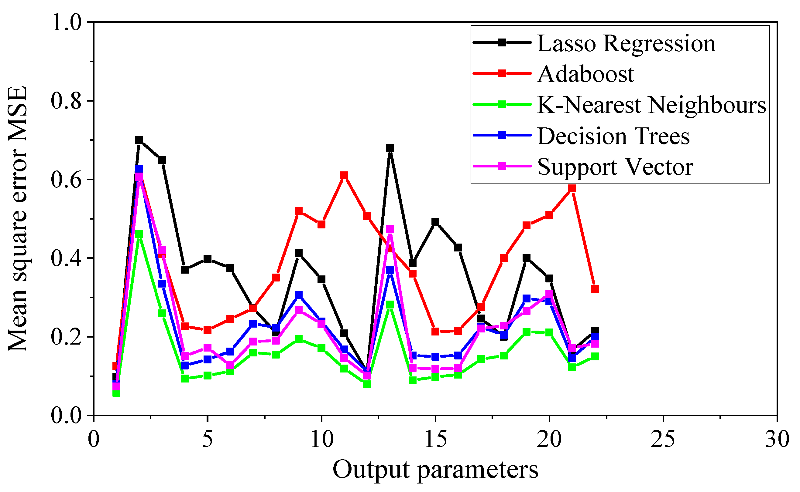
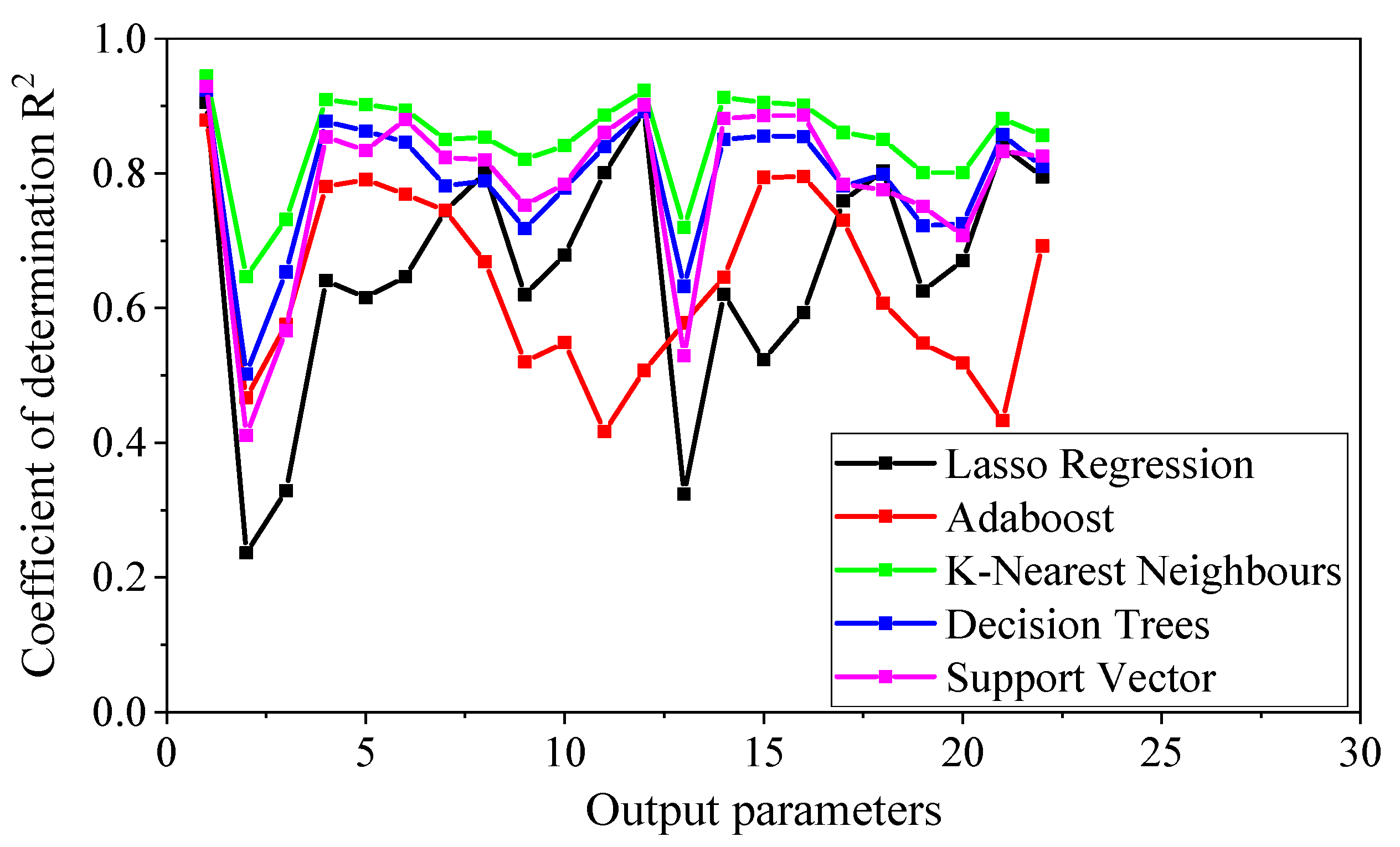
The predictive performance of various machine learning methods was systematically evaluated using mean squared error (MSE) and coefficient of determination (R²) metrics across all 22 output variables, with comparative results presented in Figure 2 and Figure 3.

As can be seen in these figures, among all machine learning algorithms, the K-nearest neighbors (KNNs) method demonstrates better performance compared to other methods, with MSE values approaching zero and R² values near unity across the output variables. For the majority of variables, R² values exceed 0.9, while MSE values remain below 0.1.

However, as further illustrated in Figure 2 and Figure 3, certain output variables show relatively lower predictive accuracy, warranting further investigation into the underlying causes. Specifically, the second, third, and thirteenth output variables correspond to the shear forces at points where the displacement drift is zero, +0.1%, and −0.1%, respectively, on the skeleton curve. The prediction performance for these points is not perfect. It may be attributed to the fact that these points represent the initial zero-displacement point or the residual displacement points on the skeleton curves of columns after earthquake loading. The coordinates of these points tend to be less stable compared to other points on the skeleton curves, often oscillating between positive and negative values. Consequently, accurately predicting the coordinate values near zero displacement is more challenging.

When applying the K-nearest neighbors (KNNs) method to predict the skeleton curves of seismically damaged RC columns, the predicted peak strength values are extracted and compared with the corresponding actual values, as shown in Figure 4. In the figure, the dashed line represents the 45-degree diagonal. The results demonstrate that the KNN method achieves excellent prediction performance for peak strength, with a mean squared error (MSE) of 0.022 and a coefficient of determination (R²) of 0.978. Furthermore, most of the data points are clustered around the dashed line, indicating a strong agreement between the actual and predicted values, as well as a positive correlation between them.

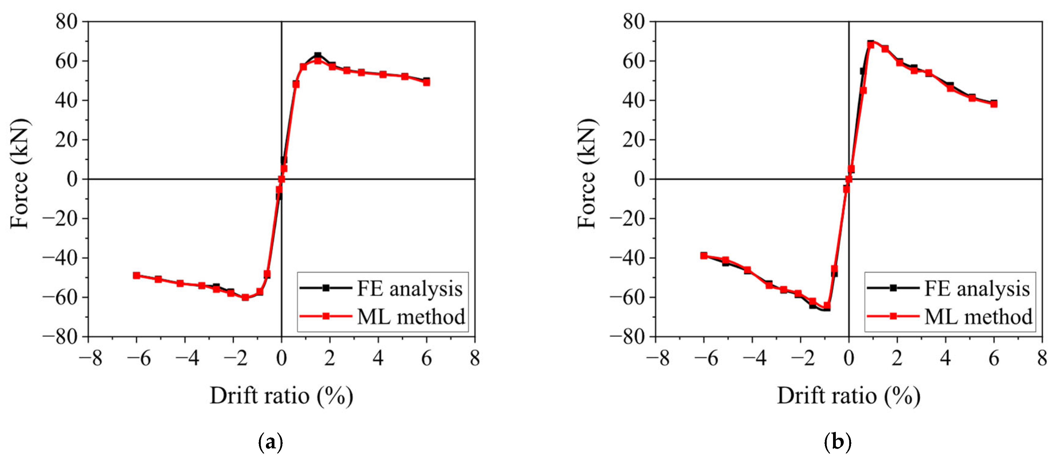
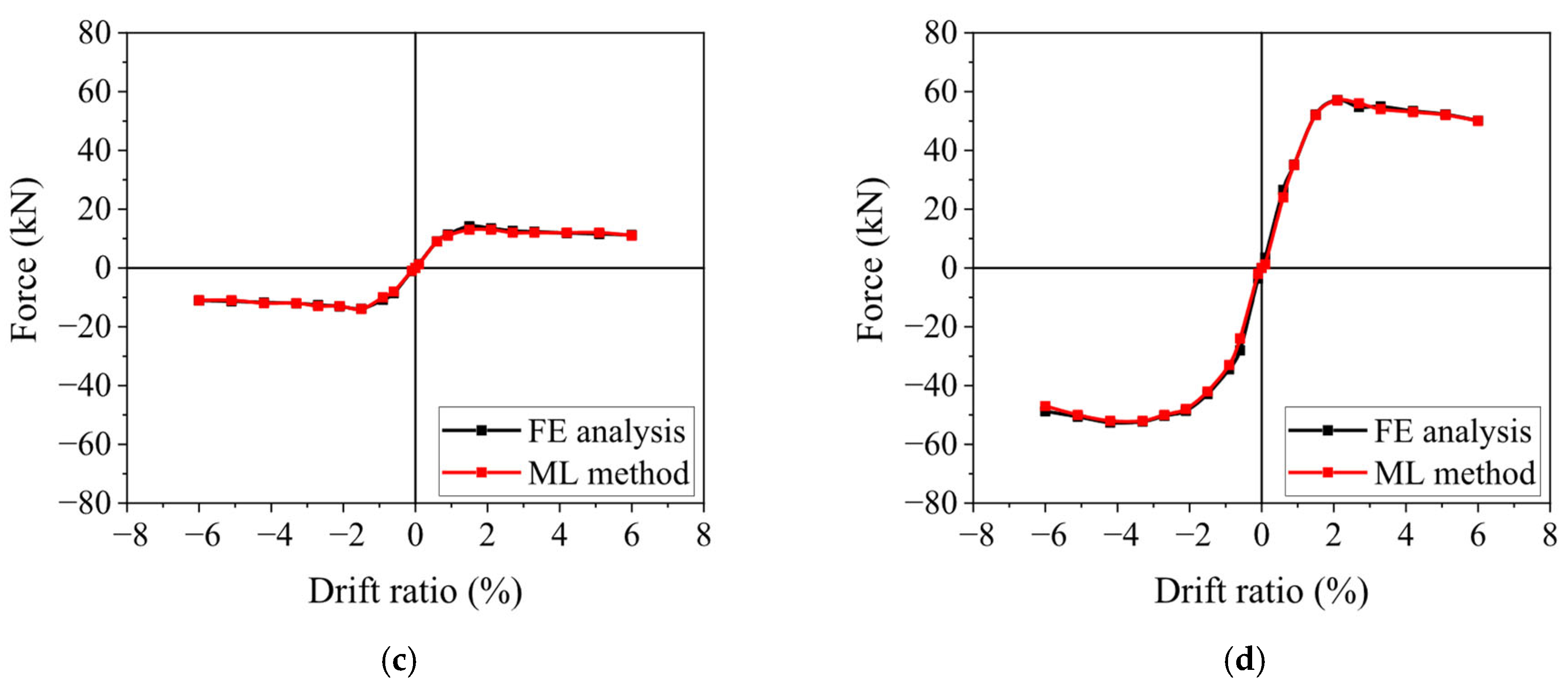
A comparison of the damaged skeleton curves predicted by K-nearest neighbors and those obtained from numerical analysis is shown in Figure 5. The results demonstrate that the K-nearest neighbors can accurately predict the skeleton curve of damaged columns, and the predicted skeleton curve aligns well with the analysis results from OpenSees. It highlights that, with sufficient sample data, the K-nearest neighbors method can produce highly satisfactory prediction results.

The damaged skeleton curves predicted by the K-nearest neighbors (KNNs) method are compared with those obtained from numerical analysis, as shown in Figure 5. The comparison demonstrates that the KNN method provides accurate predictions, with the predicted skeleton curves closely matching the results from OpenSees. It indicates that, given sufficient sample data, the KNN method is capable of delivering reliable and satisfactory prediction results.

4.2. Influence of Input Variables

It is crucial to understand which input variables have the most significant impact on predicting the damaged skeleton curves. In addition to selecting the best-performing machine learning algorithm, two methods—Principal Component Analysis (PCA) and Shapley Additive Explanations (SHAP)—were employed to evaluate the importance of each input variable to the output results.

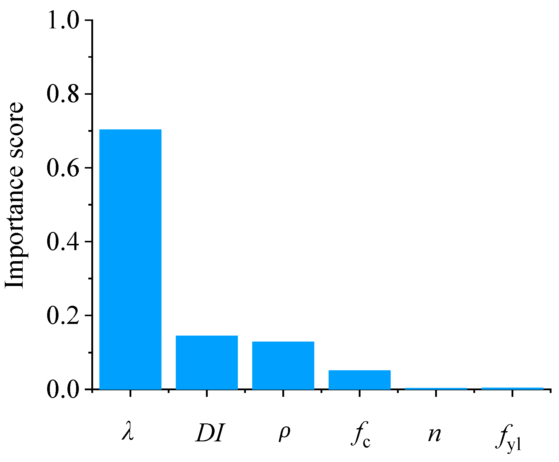
First, Principal Component Analysis (PCA), a widely used method for reducing the dimensionality of high-dimensional data, was adopted to eliminate features that had little impact on the results. By reducing the dimensionality, PCA ranks the importance of each feature. Taking the peak strength as an example, the importance scores of each input variable obtained through PCA are shown in Figure 6.

As seen in Figure 6, the importance ranking of the input features is as follows: aspect ratio, damage index, longitudinal reinforcement ratio, concrete compressive strength, yield strength of longitudinal reinforcement, and axial load ratio. The aspect ratio is the most significant factor affecting the output results, exerting a much greater influence than the other variables. The reason for these results is that the aspect ratio governs the size of the column section, and the column cross-section plays a dominant role in the column’s lateral resistance. The damage index ranks second, as expected, since the column’s bearing capacity is highly sensitive to its level of damage.

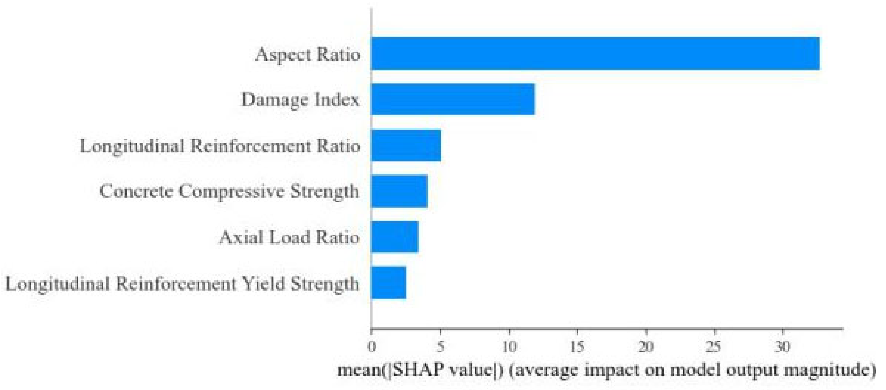
Additionally, Shapley Additive Explanations (SHAP) were applied to further explain the output of the machine learning models and to evaluate the importance of each input feature. The mean SHAP value results are presented in Figure 7, which reflect the average impact of the input variables on the output results (with peak strength as an example).

The results show that the importance rankings of input variables obtained from SHAP are almost consistent with those from PCA. The aspect ratio, followed by the damage index, is again identified as the most influential feature affecting the output results. Similarly, the other four features have relatively lower influence compared to the aspect ratio and damage index, although their importance scores differ slightly between the two evaluation methods.

4.3. Quantitative Analysis of Degradation Degree

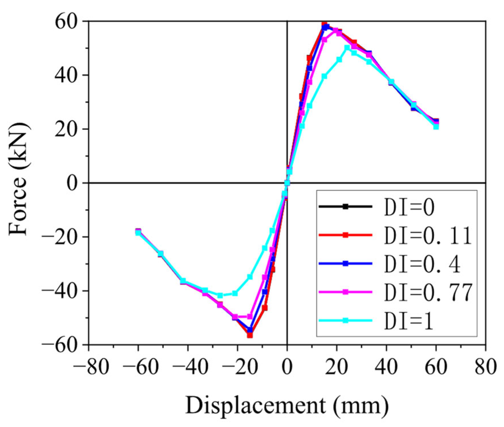
To further enhance the engineering utility and practical value of the machine learning approach, this study employs the validated KNN model as a representative example to systematically investigate the effects of damage progression on seismic behavior. Quantitative analysis of degradation degree aims to provide comprehensive insights into how skeleton curves evolve across different damage states and to generate practical engineering tools for post-earthquake assessment. Additionally, the skeleton curves at different damage levels were explored and compared to establish a comprehensive understanding of damage-induced behavioral changes. Figure 8 presents the comparison of skeleton curves across various damage levels. Taking an example with aspect ratio λ = 3, ρ_l = 1.55%, f_c = 26.8, f_yl = 400, and n = 0.2, the damage index (DI) varies from 0 to 1. The colored lines in the figure represent skeleton curves corresponding to DIs of 0, 0.11, 0.4, 0.77, and 1.0, which, respectively, correspond to intact, minor damage, moderate damage, severe damage, and collapse states. The key points shown in the figure include the zero point, yield point, peak point, and ultimate point.

As demonstrated in Figure 8, the skeleton curve for the minor damage level almost coincides with that of the intact state, suggesting that the seismic capacity of columns with minor damage is nearly equivalent to that of undamaged columns. As the damage level increases, the skeleton curves shift downward and to the right. The skeleton curves for the damaged states remain within the envelope of the intact state, clearly indicating a gradual decline in seismic capacity. The strength at the yield point decreases slightly while the yield displacement increases. At the peak point, the peak displacement gradually increases, and the degradation of peak strength becomes significantly more pronounced as the damage index increases. For the ultimate points, except for the case of maximum damage (DI = 1), the trends in ultimate strength and ultimate displacement are not particularly noticeable. However, when DI reaches 1, the ultimate strength drops sharply, and the ultimate displacement increases significantly.

Furthermore, the coordinates of the key characteristic points on the skeleton curves of RC columns at various damage levels are provided in this study and listed in

Table 4. The characteristic point coordinates of the skeleton curve of RC columns in various damage levels (λ = 3, ρ_l = 1.55%, f_c = 26.8, f_yl = 400, and n = 0.2).

DI	Damage Levels	Yield Point (kN, mm)	Peak Point (kN, mm)	Ultimate Point (kN, mm)
0	Intact	(43.93, 8.47)	(58.57, 15.00)	(46.86, 33.95)
0.11	Minor damage	(43.92, 8.50)	(58.56, 15.10)	(46.85, 33.80)
0.4	Moderate damage	(43.44, 9.37)	(57.92, 16.03)	(46.33, 34.53)
0.77	Severe damage	(42.41, 10.92)	(56.55, 19.47)	(45.24, 35.22)
1	Collapsed damage	(37.62, 13.24)	(50.16, 24.15)	(40.13, 38.36)

. These tabulated results represent a significant practical contribution, as they enable engineers to directly obtain skeleton curve parameters for damaged columns without requiring complex numerical simulations. In practical applications, when the damage state or the corresponding damage index is obtained from post-earthquake reconnaissance (such as through identification or empirical analysis), even if the damage did not necessarily result from the earthquake, the skeleton curves of columns in different damage states can still be conveniently derived from Table 4 without requiring additional calculations or simulations. The approach can also be used to evaluate the post-earthquake degradation of seismic capacity for columns at various damage levels, providing essential data for post-earthquake structural assessment and retrofitting decisions.

To provide a more detailed investigation of the residual seismic capacity of RC columns, the degradation ratios of strength and stiffness at different damage levels are presented in

Table 5. Seismic degradation ratios of RC columns in various damage levels.

DI	Damage Levels	Degradation Ratio of Strength γ1	Degradation Ratio of Stiffness γ2
0	Intact	100%	100%
0.11	Minor damage	99.9%	99.6%
0.4	Moderate damage	98.8%	89.4%
0.77	Severe damage	96.5%	74.9%
1	Collapsed damage	85.6%	54.8%

. From Table 5, it can be observed that for the minor damage level (DI = 0.11), the degradation of strength and stiffness is minimal. However, at the most severe damage level (i.e., collapse), the strength degradation ratio reaches 85.6%, while the stiffness degradation ratio is approximately 50%.

5. Conclusions

This study developed a comprehensive machine learning framework for predicting the skeleton curves of earthquake-damaged reinforced concrete columns, addressing a critical gap in post-earthquake structural assessment. The investigation utilized an extensive database derived from 1350 column models subjected to 250 seismic loading scenarios. Six input parameters were employed, with damage index as a key innovation, to predict 22 output variables representing complete skeleton curve coordinates and degradation parameters. Five machine learning algorithms were systematically evaluated. The main work and key conclusions are as follows:

• The research developed an extensive database comprising numerical simulations from common-size column models across all damage levels.
• A machine learning model was developed that predicted the skeleton curve of RC columns as a direct function of their pre-existing damage level, quantified by the damage index, enabling damage-informed prediction of residual structural performance. Machine learning demonstrated excellent ability to predict skeleton curves, particularly in the yielding and descending branches, though prediction performance for coordinate values near zero displacement was less accurate.
• Among the five machine learning algorithms evaluated, K-nearest neighbors achieved the best performance with exceptional accuracy (R² = 0.978, MSE = 0.022 for peak strength prediction). The approach could reconstruct entire damaged skeleton curves through 22 characteristic points, providing a comprehensive assessment of residual strength, stiffness, and ductility.
• PCA and SHAP identified the aspect ratio as the most influential parameter, followed by the damage index. This study established comprehensive degradation relationships showing negligible capacity reduction for minor damage (DI = 0.11: 99.9% strength retention, 99.6% stiffness retention) versus severe degradation at the collapse level (DI = 1.0: 85.6% strength retention, 54.8% stiffness retention), providing practical insights for post-earthquake evaluation and retrofitting decisions.

The demonstrated efficiency of the prediction framework suggests potential for developing real-time monitoring systems and expanding applications to broader seismic scenarios. Future research should focus on expanding the ground motion database beyond the current 50 records to include near-field effects, pulse-like motions, and diverse site conditions, while extending the framework to account for cumulative damage from multiple hazards, including earthquakes, wind, and fatigue loading. These developments would further enhance the practical applicability of ML-based approaches in post-earthquake structural assessment and contribute to more resilient infrastructure systems.

References

1. Naderpour, H.; Mirrashid, M. Proposed soft computing models for moment capacity prediction of reinforced concrete columns. Soft Comput. 2020, 24, 11715–11729. [Google Scholar] [CrossRef]
2. Ning, C.-L.; Wang, L.; Du, W. A practical approach to predict the hysteresis loop of reinforced concrete columns failing in different modes. Constr. Build. Mater. 2019, 218, 644–656. [Google Scholar] [CrossRef]
3. Luo, H.; Paal, S.G. A locally weighted machine learning model for generalized prediction of drift capacity in seismic vulnerability assessments. Comput. Civ. Infrastruct. Eng. 2019, 34, 935–950. [Google Scholar] [CrossRef]
4. Xie, Y.; Ebad Sichani, M.; Padgett, J.E.; Desroches, R. The promise of implementing machine learning in earthquake engineering: A state-of-the-art review. Earthq. Spectra 2020, 36, 1769–1801. [Google Scholar] [CrossRef]
5. Asim, K.M.; Martínez-Álvarez, F.; Basit, A.; Iqbal, T. Earthquake magnitude prediction in Hindukush region using machine learning techniques. Nat. Hazards 2016, 85, 471–486. [Google Scholar] [CrossRef]
6. Xiong, C.; Li, Q.; Lu, X. Automated regional seismic damage assessment of buildings using an unmanned aerial vehicle and a convolutional neural network. Autom. Constr. 2020, 109, 102994. [Google Scholar] [CrossRef]
7. Balz, T.; Liao, M. Building-damage detection using post-seismic high-resolution SAR satellite data. Int. J. Remote. Sens. 2010, 31, 3369–3391. [Google Scholar] [CrossRef]
8. Jiang, Y.; Yang, G.; Song, H. Dynamic optimization design of extradosed cable-stayed bridge under earthquake excitation. Eng. Mech. 2020, 37, 313–319. [Google Scholar] [CrossRef]
9. Pang, Y.; Dang, X.; Yuan, W. An Artificial Neural Network Based Method for Seismic Fragility Analysis of Highway Bridges. Adv. Struct. Eng. 2014, 17, 413–428. [Google Scholar] [CrossRef]
10. Giovanis, D.G.; Fragiadakis, M.; Papadopoulos, V. Epistemic uncertainty assessment using Incremental Dynamic Analysis and Neural Networks. Bull. Earthq. Eng. 2015, 14, 529–547. [Google Scholar] [CrossRef]
11. Su, L.; He, H.-J. Decision tree–based seismic damage prediction for reinforcement concrete frame buildings considering structural micro-characteristics. Adv. Struct. Eng. 2019, 22, 2097–2109. [Google Scholar] [CrossRef]
12. Kia, A.; Sensoy, S.; Xie, X. Classification of Earthquake-Induced Damage for R/C Slab Column Frames Using Multiclass SVM and Its Combination with MLP Neural Network. Math. Probl. Eng. 2014, 1, 734072. [Google Scholar] [CrossRef]
13. Morfidis, K.; Kostinakis, K. Seismic parameters’ combinations for the optimum prediction of the damage state of R/C buildings using neural networks. Adv. Eng. Softw. 2017, 106, 1–16. [Google Scholar] [CrossRef]
14. Morfidis, K.; Kostinakis, K. Approaches to the rapid seismic damage prediction of r/c buildings using artificial neural networks. Eng. Struct. 2018, 165, 120–141. [Google Scholar] [CrossRef]
15. Morfidis, K.; Kostinakis, K. Comparative evaluation of MFP and RBF neural networks’ ability for instant estimation of r/c buildings’ seismic damage level. Eng. Struct. 2019, 197, 109436. [Google Scholar] [CrossRef]
16. Harirchian, E.; Jadhav, K.; Kumari, V.; Lahmer, T. ML-EHSAPP: A prototype for machine learning-based earthquake hazard safety assessment of structures by using a smartphone app. Eur. J. Environ. Civ. Eng. 2021, 26, 5279–5299. [Google Scholar] [CrossRef]
17. Zhang, Y.; Burton, H.V.; Sun, H.; Shokrabadi, M. A machine learning framework for assessing post-earthquake structural safety. Struct. Saf. 2018, 72, 1–16. [Google Scholar] [CrossRef]
18. Mangalathu, S.; Sun, H.; Nweke, C.C.; Yi, Z.; Burton, H.V. Classifying earthquake damage to buildings using machine learning. Earthq. Spectra 2020, 36, 183–208. [Google Scholar] [CrossRef]
19. Palanci, M. Fuzzy rule based seismic risk assessment of one-story precast industrial buildings. Earthq. Eng. Eng. Vib. 2019, 18, 631–648. [Google Scholar] [CrossRef]
20. Han, X.; Wu, Z.; Yang, M.; Ji, J. Research on seismic damage assessment of regional RC frame structures based on deep learning. J. Build. Struct. 2020, 41, 27–35. [Google Scholar] [CrossRef]
21. Han, X.; Feng, R.; Ji, J.; Wu, Z. Research on parameters of the RC beam lumped plastic hinge model based on deep learning. Eng. Mech. 2021, 38, 160–169. [Google Scholar] [CrossRef]
22. Di Ludovico, M.; Polese, M.; D’aRagona, M.G.; Prota, A.; Manfredi, G. A proposal for plastic hinges modification factors for damaged RC columns. Eng. Struct. 2013, 51, 99–112. [Google Scholar] [CrossRef]
23. Li, L.; Luo, G.; Wang, Z.; Zhang, Y.; Zhuge, Y. Prediction of residual behaviour for post-earthquake damaged reinforced concrete column based on damage distribution model. Eng. Struct. 2021, 234, 141–296. [Google Scholar] [CrossRef]
24. Todorov, B.; Billah, A.M. Post-earthquake seismic capacity estimation of reinforced concrete bridge piers using Machine learning techniques. Structures 2022, 41, 1190–1206. [Google Scholar] [CrossRef]
25. Valente, M. Seismic Upgrading Strategies for Non-Ductile Plan-Wise Irregular R/C Structures. Procedia Eng. 2013, 54, 539–553. [Google Scholar] [CrossRef]
26. Valente, M.; Milani, G. Alternative retrofitting strategies to prevent the failure of an under-designed reinforced concrete frame. Eng. Fail. Anal. 2018, 89, 271–285. [Google Scholar] [CrossRef]
27. GB50010-2010; Code for Seismic Design of Buildings. Ministry of Housing and Urban-Rural Development of P.R. China: Beijing, China, 2010.
28. Kunnath, S.K.; Reinhorn, A.M.; Lobo, R.F. A Program for the Inelastic Damage Analysis of Reinforced Concrete Structures, Version 3.0. Technical Report NCEER-92-0022. National Center for Earthquake Engineering Research, SUNY: Buffalo, NY, USA, 1992.
29. Kempton, J.J.; Stewart, J.P. Prediction Equations for Significant Duration of Earthquake Ground Motions considering Site and Near-Source Effects. Earthq. Spectra 2006, 22, 985–1013. [Google Scholar] [CrossRef]
30. Rathje, E.M.; Abrahamson, N.A.; Bray, J.D. Simplified Frequency Content Estimates of Earthquake Ground Motions. J. Geotech. Geoenviron. Eng. 1998, 124, 150–159. [Google Scholar] [CrossRef]
31. Du, W. An empirical model for the mean period (Tm) of ground motions using the NGA-West2 database. Bull. Earthq. Eng. 2017, 15, 2673–2693. [Google Scholar] [CrossRef]
32. Tibshirani, R. Regression Shrinkage and Selection Via the Lasso. J. R. Stat. Soc. Ser. B Stat. Methodol. 1996, 58, 267–288. [Google Scholar] [CrossRef]
33. Freund, Y.; Schapire, R.E. A Decision-Theoretic Generalization of On-Line Learning and an Application to Boosting. J. Comput. Syst. Sci. 1997, 55, 119–139. [Google Scholar] [CrossRef]
34. Drucker, H. Improving regressors using boosting techniques. In Proceedings of the Fourteenth International Conference on Machine Learning 1997, Nashville, TN, USA, 8–12 July 1997; pp. 107–115. [Google Scholar]
35. Cover, T.; Hart, P. Nearest neighbor pattern classification. IEEE Trans. Inf. Theory 1967, 13, 21–27. [Google Scholar] [CrossRef]
36. Breiman, L.; Friedman, J.; Stone, C.J.; Olshen, R.A. Classification and Regression Trees; Chapman and Hall/CRC: Boca Raton, FL, USA, 2017. [Google Scholar]
37. Vapnik, V. The Nature of Statistical Learning Theory; Springer: New York, NY, USA, 1995. [Google Scholar]
38. Bergstra, J.; Bengio, Y. Random search for hyper-parameter optimization. J. Mach. Learn. Res. 2012, 13, 281–305. [Google Scholar]
39. Belete, D.M.; Huchaiah, M.D. Grid search in hyperparameter optimization of machine learning models for prediction of HIV/AIDS test results. Int. J. Comput. Appl. 2021, 44, 875–886. [Google Scholar] [CrossRef]
Figure 1. Sketch diagram of targeted output coordinate points on skeleton curves.
Buildings 15 03135 g001
Figure 2. The mean square error MSE of each output variable for different machine learning methods.
Buildings 15 03135 g002
Figure 3. The coefficient of determination R-Squared R2 of each variable for different machine learning methods.
Buildings 15 03135 g003
Figure 4. Peak strength distribution diagram predicted by the K-nearest neighbors method.
Buildings 15 03135 g004
Figure 5. Comparison between prediction results and numerical analysis results of skeleton curves of seismically damaged columns. (a) λ = 2, ρl = 1.15%, fc = 23.4, fyl = 500, n = 0.3, DI = 0.1; (b) λ = 2, ρl = 1.55%, fc = 26.8, fyl = 500, n = 0.8, DI = 0.4; (c) λ = 3, ρl = 1.15%, fc = 20.1, fyl = 400, n = 0.2, DI = 0.29; (d) λ = 2, ρl = 1.15%, fc = 23.4, fyl = 500, n = 0.3, DI = 0.86.
Buildings 15 03135 g005aBuildings 15 03135 g005b
Figure 6. Importance ranking of input variables by the PCA method (taking peak strength as an instance).
Buildings 15 03135 g006
Figure 7. Importance ranking of input variables by the SHAP method (taking peak strength as an instance).
Buildings 15 03135 g007
Figure 8. Comparison of skeleton curves of RC columns in various damage levels.
Buildings 15 03135 g008