Article

The Hydrogen Trade-Off: Optimizing Decarbonization Pathways for Urban Integrated Energy Systems

1
School of Thermal Engineering, Shandong Jianzhu University, Jinan 250101, China
2
Sichuan Institute of Building Research, Chengdu 610084, China
*
Author to whom correspondence should be addressed.
Buildings 2025, 15(17), 3014; https://doi.org/10.3390/buildings15173014 (registering DOI)
Submission received: 16 July 2025 / Revised: 8 August 2025 / Accepted: 22 August 2025 / Published: 25 August 2025
(This article belongs to the Special Issue Potential Use of Green Hydrogen in the Built Environment)

Abstract

Rapid socio-economic development has made energy application and environmental issues increasingly prominent. Hydrogen energy, clean, eco-friendly, and highly synergistic with renewable energy, has become a global research focus. This study, using the EnergyPLAN model that includes the electricity, transportation, and industrial sectors, takes Jinan City as the research object and explores how hydrogen penetration changes affect the decarbonization path of the urban integrated energy system under four scenarios. It evaluates the four hydrogen scenarios with the entropy weight method and technique, placing them in an order of preference according to their similarity to the ideal solution, considering comprehensive indicators like cost, carbon emissions, and sustainability. Results show the China Hydrogen Alliance potential scenario has better CO2 emission reduction potential and unit emission reduction cost, reducing them by 7.98% and 29.39%, respectively. In a comprehensive evaluation, it ranks first with a score of 0.5961, meaning it is closest to the ideal scenario when cost, environmental, and sustainability indicators are comprehensively considered. The Climate Response Pioneer scenario follows with 0.4039, indicating that higher hydrogen penetration in terminal energy is not necessarily the most ideal solution. Instead, appropriate hydrogen penetration scenarios should be selected based on the actual situation of different energy systems.

1. Introduction

In recent years, climate disasters such as increased global warming, frequent occurrences of extreme weather, the oil crisis, and nuclear accidents have triggered a profound reflection on the transformation of the energy mix [1]. Under the dual drive of global climate change and energy structure transformation, realizing the deep decarbonization of the integrated energy system (IES) has become a core issue in addressing environmental challenges and promoting sustainable development [2]. Hydrogen energy, as a zero-carbon energy carrier, is becoming increasingly strategic in the energy transition [3].
Hydrogen energy is at the forefront of research in the field of integrated energy systems due to its advantages; it is clean, efficient and renewable [4]. In-depth exploration of the optimal configuration of an integrated electric–hydrogen energy system is crucial to achieving net-zero emissions and managing the volatility of renewable energies. Recent studies have focused on optimizing the configuration and operation of such systems from multiple perspectives. For example, to balance the interests of multiple stakeholders, Zhang et al. [5] developed a multi-criteria decision-making framework and identified an optimal configuration for an industrial park combining natural gas, photovoltaics, and hydrogen storage, which achieved a significant 76% reduction in carbon emissions. Similarly, for achieving net-zero demand matching, Wada et al. [6] assessed a fully renewable-powered hydrogen system and concluded that while technically feasible, such projects currently require subsidies or additional revenue streams to be economically profitable, highlighting a key economic challenge. To specifically address renewable energy volatility, the integration of hydrogen storage has been proven effective. Wu et al. [7] demonstrated that configuring a system with hydrogen storage can increase the renewable energy consumption rate by 6.54% and reduce grid interaction by 45.01% compared to systems without any storage. Building on this, Xu et al. [8] further explored hydrogen’s role in a comprehensive demand response framework, showing that a coordinated power–gas–heat–hydrogen strategy can cut energy costs by 12~27%. Beyond configuration, researchers are also refining operational strategies and integrating advanced technologies. Yang et al. [9] tackled long-term supply–demand imbalances by proposing a nested optimization method, finding that integrating waste heat recovery with hydrogen storage could reduce total annual operational costs by 1.16% while significantly improving computational efficiency. Meanwhile, Wu et al. [10] proposed a coordinated planning model featuring high-temperature electrolysis powered by concentrated solar plants, developing a detailed framework to improve the overall efficiency of the power-to-hydrogen process. From a market perspective, Li et al. [11] revealed the substantial economic potential of these systems; their multi-level market model showed that by including income from hydrogen sales, the economic benefits of an IES with offshore wind could increase by as much as 205.64%.
With the rapid development and widespread application of artificial intelligence technology [12,13], a substantial body of research has focused on enhancing system efficiency and facilitating low-carbon development through the formulation of diverse optimization models and the utilization of various algorithms and mechanisms [14]. A primary focus of this research has been to develop optimization models that simultaneously minimize costs and carbon emissions, with studies reporting significant achievements. For instance, Dong et al. [15] demonstrated that a coordinated hydrogen-based IES in an industrial park could achieve a remarkable 95.44% reduction in emissions. The benefits of collaboration were further quantified by Wang et al. [16], whose cooperative game theory model showed that joint operation could reduce total costs by 22.96% and emissions by 80.11% compared to independent operation scenarios. To achieve these reductions, many studies incorporate market mechanisms and advanced technologies. Yang et al. [17] employed a ladder-type carbon trading mechanism and demand response, resulting in a 3.56% operational cost reduction and a 5.44% increase in Photo Voltaic (PV) consumption. Similarly, Zhan et al. [18] integrated fuel cell waste heat recovery with a tiered carbon trading model, leading to a 30.7% total cost reduction and an 18.8% decrease in carbon emissions. Beyond general optimization, researchers are tackling specific operational complexities and uncertainties. Sohani et al. [19] highlighted the critical impact of component degradation, showing that accounting for performance loss could necessitate increasing PV and electrolyzer capacities by over 11% and 38%, respectively, to meet system targets. To manage temporal challenges, Liu et al. [20] introduced a two-layer model with seasonal hydrogen storage, demonstrating its effectiveness in leveraging seasonal complementarities to reduce natural gas purchase costs by 9.10% under high renewable penetration. To handle real-time uncertainties, Fang et al. [21] proposed a multi-stage, multi-timescale energy management framework, proving its economic benefits in a system with inter-microgrid hydrogen trading. Furthermore, the state of the art includes advanced algorithmic contributions and strategic market analysis. Judge et al. [22], for example, developed an improved metaheuristic algorithm that outperformed several existing methods and designed a hybrid system projected to avoid 72.05% of carbon emissions. From a market investment perspective, Joseph et al. [23] used a game-theoretic model to analyze a liberalized energy market, concluding that a round-trip efficiency of at least 50% is crucial for the profitability of vector-coupling storage and quantifying its advantages over Li-ion batteries.
At present, the research on hydrogen energy in integrated energy systems is mostly limited to green hydrogen power generation and energy storage scenarios, with insufficient depth of scenario design, a lack of quantitative analysis of sub-gradient penetration rate, and neglect of the decarbonization potentials of terminal areas such as industrial fuel substitution and transportation energy transformation. These matters have not been fully explored, which results in the serious underestimation of the overall contribution of hydrogen energy to the integrated energy system. The overall contribution of hydrogen energy to the integrated energy system has been seriously underestimated, and the focus is mostly on a single sector of power or transportation, ignoring the synergistic effect between industry, transportation, and power systems, which makes it difficult to demonstrate the coupling characteristics of the integrated energy system and restricts the exploration of the overall optimization path of the system. Therefore, based on EnergyPLAN, we constructed a model of an integrated energy system coupled with the electric power, transportation, and industrial sectors, constructed four end-use energy penetration scenarios, and quantified the demand for hydrogen under different scenarios, which provides a more comprehensive assessment path for an integrated energy system to realize deep decarbonization at a cross-regional scale.

2. Energy Development Modeling

2.1. Model Building

The integrated energy system encompasses coal, oil, natural gas, electricity, heat, wind, and solar energy, which support economic and social operations. It has been transformed from a “traditional structure centered on a single network” to an “integrated system centered on electricity”, and the key to the transformation lies in the coordination of multisectoral supply and demand activities and the synergistic promotion of the efficient integration of traditional fossil energy sources and new clean energy sources [24]. Due to the seasonality and volatility of renewable energy, it is necessary to rely on hourly or even smaller scale time data to accurately characterize the annual output and energy use behavior of the system.

2.1.1. Modeling Framework

EnergyPLAN is an energy system analysis model developed by Aalborg University in Denmark, specifically designed for technical–economic simulation of multi-sector coupled systems such as electricity, industry, and transportation [25]. The model employs a deterministic input–output framework with hourly resolution [26], simulating the system’s annual operation based on user-inputted energy demand, renewable energy availability, technical costs, and other parameters, and outputting key indicators such as fuel consumption, carbon emissions, and total system costs. Its primary function is to conduct scenario comparison analyses to evaluate the comprehensive benefits of different energy strategies. However, the model also has limitations, primarily that it is a simulation tool rather than an optimization model and cannot automatically optimize solutions. Additionally, it simplifies the power grid into a single-node model without considering network congestion, so its analysis focuses on overall system balance rather than specific grid operation details. The constructed reference model framework is shown in Figure 1.

2.1.2. Mathematical Expression

i.
Electricity sector
The electricity sector is the core of the integrated energy system. The annual electricity demand of a region is the sum of the hourly electricity demands of various sectors. In order to cover a longer time period in the analysis and consider the minor impact that leap years may have, this study selected leap years as typical analysis years, with a total duration of 8784 h [25], as shown in Equation (1).
P e l = n = 1 8784 p e l ( n )
where Pel is the annual electricity demand; pel is the hourly electricity demand; and 8784 is the total leap year hours.
For renewable energy sources, the calculation function for power generation is shown in Equation (2).
P r e s = ε C r e s Q r e s m a x ( Q r e s )
where Pres is the renewable energy generation capacity; ε is the correction factor between capacity and production; Cres is the installed renewable energy generation capacity; and Qres is the distribution of electricity production under the 8784 h benchmark.
ii.
Transportation sector
The fuel demand in the transportation sector is intended to describe the potential changes in the sector, and there is no hourly distribution data for fuel demand within the model, which is calculated as a functional equation as shown in Equation (3).
P t r a n s = P d i + P p e + P j p + P h y
where Ptotal is the total fuel demand in the transportation sector, Pdi is the diesel demand, Ppe is the gasoline demand, Pjp is the jet fuel demand, and Phy is the hydrogen demand.
iii.
Industry sector
Fuel consumption in the industrial sector takes into account the demand for coal, oil, and natural gas as well as biomass, which is calculated as a function of Equation (4) [27].
P i n = P c o + P o i l + P n a + P b i
where Pin is the industry sector fuel demand, Pco is the coal demand, Poil is the fuel oil demand, Pna is the natural gas demand, and Pbi is the biomass demand.

2.2. Energy Forecasting Model

2.2.1. Energy Demand Projections

This paper employs a time series-based multiple linear regression (MLR) method. MLR is a classic statistical analysis technique that aims to quantify the relationship between a dependent variable and multiple independent variables by establishing a linear equation. This method not only explains historical data but also makes predictions based on future scenarios of the independent variables. First, based on economic and social development theory, we selected macroeconomic and social development indicators closely related to energy consumption as potential independent variables, constructing the following initial theoretical model (5) [28].
l n P i = a + b 1 l n G D P + b 2 l n P o p + b 3 l n S e c + b 4 l n U r b + b 5 l n E t e
where Pi is the energy demand, GDP is the GDP per capita, Pop is the population size, Sec is the share of secondary industry, Urb is the rate of urbanization, Ete is the consumer price index, and a, b1, b2, b3, b4, and b5 are the model parameters.
We collected historical indicator data for Jinan City, sourced from the “Jinan City Statistical Yearbook.” Subsequently, we used the statistical analysis software Statistical Package for the Social Sciences Statistics 27, which is distributed by IBM Corp (IBM SPSS Statistics 27) to solve the model parameters. Through regression analysis, we tested the explanatory power of each independent variable on the dependent variable and its statistical significance (typically measured by the p-value) and excluded non-significant variables to ultimately determine the optimal predictive model [29]. The detailed regression analysis process, data sources, and results verification are presented in Appendix A.

2.2.2. Renewable Energy Supply Projections

To make a prediction of the future renewable energy supply, mainly for Jinan City, we combined the potential of wind power, photovoltaic, and biomass with policy planning data and our scenario analysis method to predict the future installed capacity, assuming that the installed capacity from 2025 to the policy planning year will follow a path of linear growth. The resulting prediction model is shown in Equation (6).
C y = C 2025 + Q 5 C 2025 5 × y ,   0 y 5 C y = C 2025 + Q 10 C 2025 10 × y ,   5 y 10
where Cy is the installed capacity after year y, C2025 is the installed capacity in the base year, Q5 is the policy planning installed capacity target after 5 years, Q10 is the policy planning installed capacity target after 10 years, and y is the forecast year.

3. Hydrogen Energy Scenario Penetration Modeling

3.1. Modeling of Hydrogen End-Use Energy Penetration

Hydrogen energy needs more than ten years or even decades to be deeply integrated into the existing energy structure [30]. The sectors with high hydrogen energy penetration such as electric power, industry, and transportation were selected to be analyzed, and the scenario application analysis model was constructed based on the end-use energy penetration rate of hydrogen energy. Based on the energy demand and renewable energy supply prediction model, the development path of an integrated energy system in Jinan City in the coming 10 years under the basic scenario was simulated, as well as its end-use energy consumption. According to the output of the BEIS scenario simulation, the terminal energy consumption is shown by Equation (7).
F T C = E y E x p y + I m p y + i j f F T C , y , i , j
where FTC is the final energy consumption, Ey is the total electricity production, Expy is the exported electricity, Impy is the imported electricity, fFTC is the final fuel consumption, with subscript i for the energy-using sector and subscript j for the fuel type, and y is the year of simulation.
The amount of hydrogen used for each hydrogen energy scenario is shown in Equation (8).
H t o t a l , n = γ n × F T C y n = { C R P S , Q P D S , C H A P S }
where Htotal,n is the total annual hydrogen use and γy,n is the hydrogen end-use energy penetration rate.
i.
Modeling hydrogen penetration in the electricity sector
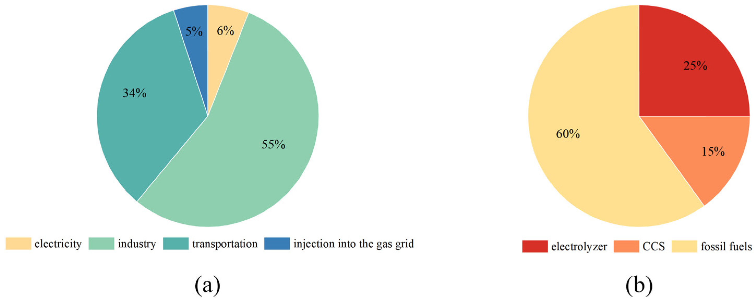
Hydrogen penetration in the electricity sector is mainly realized through gas turbine hydrogen doping [31] and coal power doping. The amount of fuel replaced by hydrogen is shown in Equations (10) and (11). The proportion of hydrogen in each of the demand–supply distribution application scenarios is shown in Figure 2.
H e l e c = α e l e c × H t o t a l , n
M e l e c , n g = H e l e c × β e l e c × μ n g
M e l e c , c o = H e l e c × β e l e c × μ c o
where Helec is the total hydrogen usage in the electricity sector, Melec,ng is the hydrogen blending ratio for gas turbines, Melec,co is the hydrogen blending ratio for coal-fired power generation, αelec is the percentage of hydrogen demand in the electricity sector, βelec is the percentage of hydrogen supply in the electricity sector, μng is the hydrogen substitution capacity for gas, which takes the value of 50%, and μco is the hydrogen substitution capacity for coal, which takes the value of 50%.
ii.
Modeling hydrogen penetration in the industry sector
Hydrogen penetration in the industry sector is mainly realized by substituting hydrogen for coal and natural gas. In order to simplify the analysis process, the substitution of natural gas in the industry sector is realized through hydrogen injection into the gas network. The amount of fuel that is replaced by hydrogen is shown in Equations (13)–(15).
H I n d = α I n d × H t o t a l , n
M I n d = H I n d × β I n d
H i n j = α i n j × H t o t a l , n
M i n j = H i n j × β i n j
where HInd is the total hydrogen use in the industry sector, αInd is the hydrogen demand share in the industry sector, and βInd is the hydrogen supply share in the industry sector. Hinj represents the total hydrogen consumption in the natural gas network, αinj represents the proportion of hydrogen demand in the gas network, βinj represents the proportion of hydrogen supply in the gas network, MInd represents the amount of hydrogen-based alternative fuels in the industrial sector, and Minj represents the amount of hydrogen-based alternative fuels replacing natural gas in the gas network.
iii.
Modeling hydrogen penetration in the transportation sector
Based on the difficulty of substituting hydrogen for different fuels in the transportation sector, the study considers only the substitution of diesel and gasoline. The amount of diesel and gasoline that is replaced by hydrogen in this sector is shown in Equations (17) and (18).
H t r a n s = α t r × H t o t a l , n
M t r , d i = H t r a n s × β t r × θ d i
M t r , p e = H t r a n s × β t r × θ p e
where Mtr,di is the amount of hydrogen replacing diesel fuel, Mtr,pe is the amount of hydrogen replacing gasoline, Htrans is the total hydrogen use in the transportation sector, αtr is the percentage of hydrogen demand in the transportation sector, βtr is the percentage of hydrogen supply in the transportation sector, θdi is the hydrogen substitution capacity for diesel fuel, which takes the value of 60%, and θpe is the hydrogen substitution capacity for gasoline, which takes the value of 40%.

3.2. Hydrogen Energy Application Scenario Construction

i.
Basic energy inertia scenario (BEIS)
As a comparison to the “inertia development” characteristic of the benchmark, assuming that Jinan maintains its current energy structure (coal-based power generation, zero application of hydrogen), the development path of the integrated energy system for the next 10 years was simulated, and the carbon emission intensity of the outgoing electricity remained unchanged. This was used to highlight the marginal improvement effect of hydrogen on the peak carbon pathway in the other scenarios.
ii.
Climate response pioneer scenario (CRPS)
The International Energy Agency (IEA) “Zero Emissions 2050: A Roadmap for the Global Energy Sector” [32] proposes that hydrogen energy should account for 2% of end-use energy consumption in 2030. This percentage will need to be further increased in 2035 to support the target of a 1.5 °C temperature rise. As a core city involved in the ecological protection of the Yellow River Basin, Jinan should strictly control the production of hydrogen from fossil energy sources and focus on promoting the integration of “wind, light, hydrogen, and storage” projects, which would set the penetration rate of hydrogen energy in terminal energy at 3%.
iii.
Policy-driven scenario (QPDS)
Jinan’s hydrogen industry development plan for the pilot zone for conversion of old and new dynamics explicitly proposes to build a 100-billion hydrogen industry cluster by 2035 and to construct a 20-square-kilometer “China Hydrogen Valley”. This goal should be supported by a significant increase in the penetration rate of hydrogen energy, which is set at 5% in terminal energy.
iv.
China Hydrogen Alliance Potential Scenario (CHAPS)
Directly related to the China Hydrogen Energy Alliance’s national forecast (5% of end-use energy by 2030), and in light of Shandong Province’s position as the core area of the “Northern Hydrogen Valley”, the penetration rate of hydrogen energy in this scenario was set at 6.5%. The input parameters for hydrogen energy penetration in 2035 for different scenarios are shown in Table 1.

4. Energy Evaluation Modeling

4.1. Construction of Evaluation Indicators

i.
Economic indicators
The total cost is used as the core economic indicator in integrated energy systems [33], which directly reflects the economics of system planning and operation and is a key constraint in balancing environmental and energy objectives. It is calculated as shown in Equation (19).
A T C = y A T C = y ( C i n v + C o s m + C e )
where ATC′ is the cumulative cost, ATC is the total annual cost, Cinv is the initial investment cost, Co&m is the fixed O&M cost; Ce is the energy cost, and y is the year.
Furthermore, to quantitatively assess the magnitude of the annual cost difference between the hydrogen penetration scenarios and the baseline scenario, especially when visual comparisons may not be remarkable, this study employs the root mean square error (RMSE). RMSE provides a single, aggregate measure of the deviation between two time-series datasets [34]. It is calculated as shown in Equation (20).
R M S E = 1 n t = 1 n ( A T C h y d r o , t A T C B E I S , t ) 2
where RMSE is the root mean square error of the cost, ATChydro,t is the annual total cost for a given hydrogen scenario in year t, ATCBEIS,t is the annual total cost for the BEIS scenario in year t, and n is the total number of years in the simulation period.
ii.
Environmental indicators
The environmental objective of the integrated energy system is to reduce the emission of greenhouse gases, especially carbon dioxide, which is evaluated in terms of the total annual carbon emissions of the system. These emissions include those from fuel combustion and from hydrogen production. Notably, our model incorporates emissions from coal-to-hydrogen production coupled with Carbon Capture and Storage [35]. This strategy is designed to scale up hydrogen supply in the initial decades, thereby avoiding exclusive reliance on more expensive green hydrogen produced via electrolysis. It is calculated as shown in Equation (21). The CO2 emission factors for fuel combustion, as listed in Table 2, were sourced from internationally recognized guidelines to ensure accuracy [36].
C E V = y C E V y = y [ i f u e l i × σ i + ( C O 2 , p r o C O 2 , C C S ) ]
where CEV′ is the cumulative carbon emissions, CEV is the annual carbon emissions, fuel is the fuel consumption, σ is the fuel carbon emission factor, CO2,pro is the carbon dioxide produced by hydrogen production from coal, CO2,ccs is the carbon dioxide captured by the combination of effective carbon reduction technologies (CCS), y denotes the year, and i denotes the fuel type.
iii.
Technical indicators
With the increase of installed renewable energy capacity in the integrated energy system, the energy consumption capacity is insufficient, resulting in the phenomenon of wind and light abandonment. The cumulative Critical Excess Electricity Production (CEEP) [37] and cumulative Renewable Energy Sources (RES) are used as the technical evaluation indexes. RES is used to measure the penetration rate of renewable energy sources and CEEP is used to measure the capacity of renewable energy consumption, and the calculation method is shown in Equations (22) and (23).
C E E P = y C E E P y = y ( P r e s P E l H i )
R E S = y P r e s
where CEEP′ is the cumulative critical excess power, CEEP is the annual critical excess power, Pres is the annual renewable power generation, PEl is the total annual power demand, Hi is the electrolyzer power consumption, and RES is the cumulative renewable power generation.

4.2. Empowerment Ranking Model Construction

4.2.1. Entropy Weight Method

The entropy weight method is an objective assignment method that determines weights based on the degree of dispersion of the indicator data [38]. The greater the data discrepancy, the smaller the entropy value and the higher the weight, which can reduce subjective bias and can handle multi-indicator evaluation. The mathematical model and calculation steps are shown below.
i.
Establish the original matrix [Xij]m×n with n evaluation objects and m evaluation indicators.
ii.
To eliminate the influence of dimensions, all indicators are first standardized. For positive indicators Yij+ and negative indicators Yij, the maximum–minimum value standardization method is typically used to map them to the [0, 1] interval.
Y i j + = Y i j m i n ( Y j ) max Y j m i n ( Y j )
Y i j = max Y j Y i j max Y j m i n ( Y j )
where Yij represents the value of the ith evaluation object in the jth evaluation indicator.
iii.
We need to calculate the indicator weight Dij and perform data translation. If the standardized data contains a value of 0 for Yij, this will result in a weight Dij of 0, rendering the entropy calculation meaningless. To ensure that all logarithmic values are meaningful, we perform a slight “translation” on the data, i.e., add a very small positive number d to all data.
D i j = Y i j + d j = 1 n ( Y i j + d ) ,   d = 0.001
iv.
Information entropy qj is a measure of information uncertainty. According to the definition of information theory, the formula for calculating the information entropy of the jth indicator is shown in Equation (27).
q j = k i = 1 n D i j ln D i j , k = 1 l n ( n )
v.
Perform the weight calculation as shown in Equation (28).
w j = 1 q i j = 1 n ( 1 q i )

4.2.2. Technique for Order Preference by Similarity to Ideal Solution (TOPSIS) Decision Theory

TOPSIS is a multi-indicator decision-making method. It ranks the objects by calculating the distance of each evaluation object from the optimal solution and the worst solution, which can objectively reflect the comprehensive advantages and disadvantages of each solution [39]. The mathematical model and calculation steps are shown below.
i.
The normalized initial matrix is constructed, in which the Euclidean quantum normalization method is used to construct the weighting method matrix and vector normalization, where each column element is divided by the current parameter of the column vectors to get the normalized normalized matrix Z.
Z i j = x i j i = 1 n x i j 2 ,   i = 1 ,   2 , ,   n ; j = 1 ,   2 , , m
In the processing of the Pareto solution set, the entire Pareto solution set constitutes the original data matrix X. The points on the Pareto front are denoted by xij, where i denotes each point located on the Pareto front and j denotes the number of dimensions on the target space.
ii.
The calculation of points and the normalization process is followed by decision-making. In decision-making, there are ideal and non-ideal points. Ideal point Z+ consists of the maximum value of the elements of each column in matrix Z, non-ideal point Z consists of the minimum value of the elements of each column in matrix Z. In deciding how to choose the best compromise program, the distance between the evaluation object and the two ideal points is considered comprehensively as an evaluation criterion. The distance between the evaluation object and the ideal point is calculated as shown in Equation (30).
d i ± = j = 1 m ω j ( Z i j Z j ± ) 2
where ωj is the weight of the jth attribute, i.e., each target weight.
The final calculation of the evaluation object and the optimal program closeness Yi, 0 < Yi < 1. The more convergent to 1, the better the evaluation object. The comprehensive evaluation parameters are shown in Equation (31).
Y i = d i d i + + d i

5. Example Results and Analysis

5.1. Results of Energy Demand Projections

Based on the multiple linear regression method constructed in the preceding section, we predicted the energy demand of the electricity, industrial, and transportation sectors in Jinan City. Referring to relevant government planning documents, the development experience of developed countries, and related research, we set the average annual growth rates of the independent variables for the policy scenarios over the next decade. Thus, the parameters were set as shown in Table 3 [40,41]. The robustness of these policy targets is corroborated by independent sources, including China’s economic growth forecast [42] and macroeconomic studies on China’s carbon neutrality pathways [43]. Using Equation (5) as the initial model, variable screening was conducted in IBM SPSS Statistics 27 to exclude independent variables with insignificant effects on the dependent variable, ultimately yielding optimized prediction models for each sector. The detailed regression statistical results for each model, including regression coefficients, significance levels, and R2 values, are fully listed in Appendix A.
i.
Electricity energy demand forecasting model
After regression analysis, the significant independent variables ultimately included in the electricity demand prediction model were per capita GDP, the proportion of secondary industry, urbanization rate, and consumer price index. The resulting prediction model is shown in Equation (32) below, with an adjusted R2 of 0.986, indicating a high degree of model fit.
l n D E l = 24.002 + 0.193 l n G D P + 1.378 l n S e c + 8.783 l n U r b 3.586 l n E t e
According to Equation (32) and Table 3, the total annual demand for electricity in Jinan City in the next 10 years is predicted as shown in Figure 3. For the years 2026–2035, the overall demand for electricity shows a growth trend, and the increase is relatively flat, though the increase in 2033 is larger. With the future energy structure adjustment and further promotion of energy-saving and emission reduction technologies, the proportion of electricity in terminal energy consumption is expected to gradually increase.
ii.
Industry energy demand forecasting model
The main factors influencing industrial fuel demand are also per capita GDP, the proportion of the secondary industry, urbanization rate, and the consumer price index. The prediction model obtained from the regression analysis is shown in Equation (33) below, with an adjusted R2 of 0.980, which also has strong explanatory power.
l n D I n = 14.001 + 0.733 l n G D P + 1.093 l n S e c 0.340 l n U r b + 4.020 l n E t e
The fuel demand forecast for the industrial sector is shown in Figure 4. From the perspective of qualitative analysis, the trend of energy demand changes over the next decade will be influenced by a number of factors such as economic growth, industrial restructuring, energy conservation, and emission reduction in an upward trend, with the increase slowing down by 2029, and the share of fossil energy in the structure of industrial energy consumption is expected to decline.
iii.
Transportation Energy Demand Forecasting Model
The energy demand of the transportation sector shows the strongest correlation with per capita GDP and the urbanization rate of the permanent population. Its prediction model is shown in Equation (34) below, with an adjusted R2 of 0.982.
l n D E T = 23.071 + 1.254 l n G D P + 1.354 l n S e c 1.997 l n U r b + 4.763 l n E t e
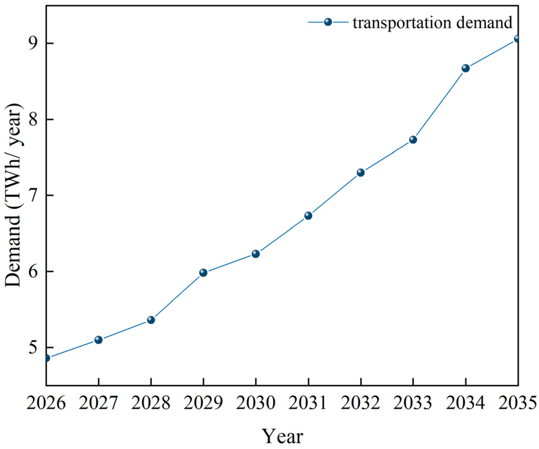
The results of the transportation sector energy demand forecast for the next 10 years are shown in Figure 5. From a qualitative analysis point of view, transportation energy demand shows a growth trend from 2026 to 2035. Gasoline and diesel, as traditional transportation energy sources, will continue to occupy an important position in the short term, with a slowing trend of growth from 2034 onwards, and their demand growth is expected to slow down due to the popularity of new energy vehicles and the optimization of the public transportation system.

5.2. Results of Renewable Energy Supply Projections

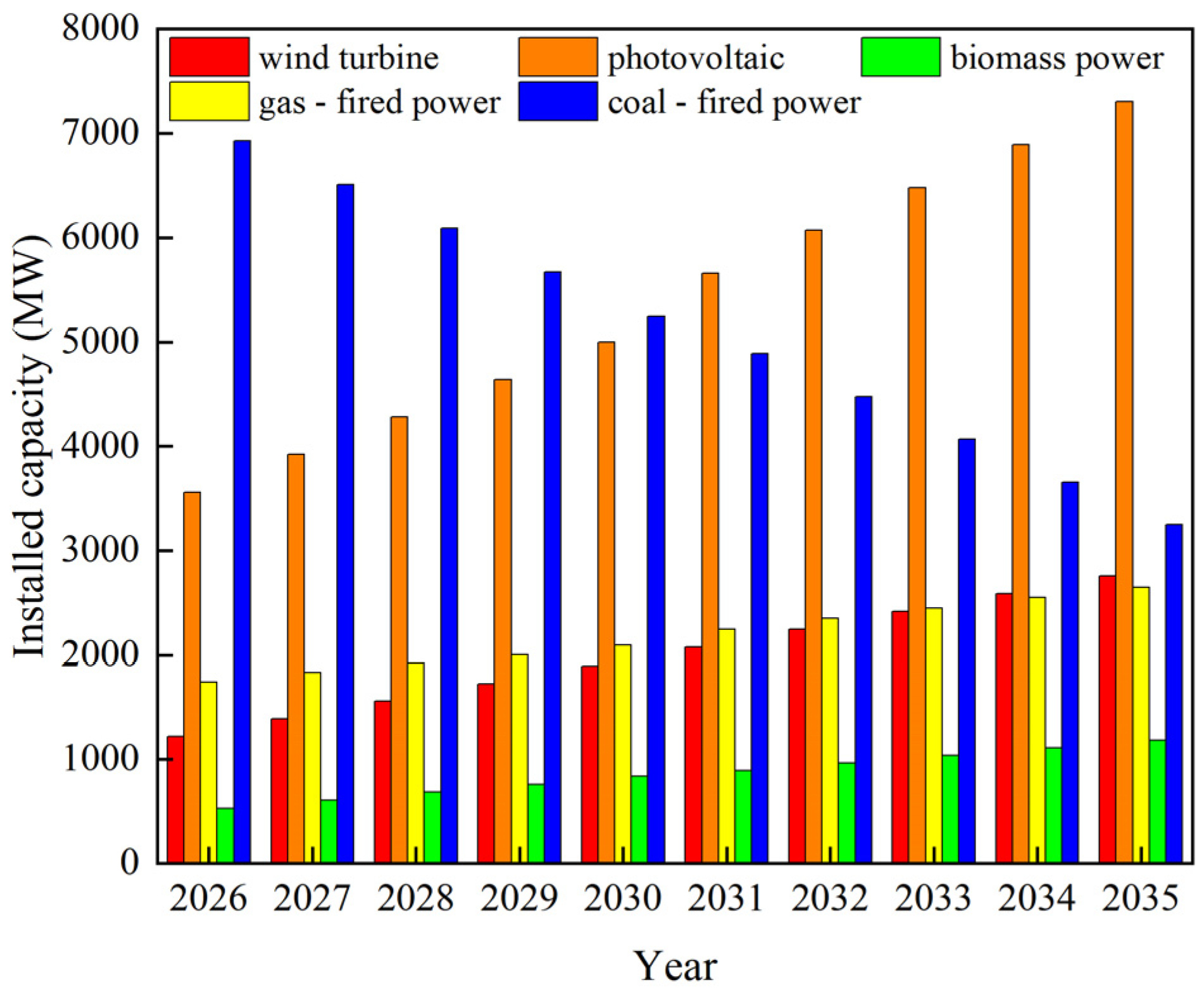
The projected growth of renewable energy capacity and the declining share of coal power are illustrated in Figure 6. The 2025 targets are based on Jinan’s “14th Five-Year Plan”. While policy-driven, these targets are well-aligned with China’s national ‘Dual Carbon’ strategy [44] and are corroborated by independent analyses. These analyses confirm the region’s high potential for solar and wind generation [45] and the compelling economic case for renewables, driven by their rapidly declining levelized cost of energy [46]. Accordingly, Figure 6 depicts the installed capacity of wind power, photovoltaics, and biomass reaching 3200 MW, 1050 MW, and 450 MW by 2025, respectively. This expansion of renewables corresponds with a projected gradual decrease in the share of coal power over the study period.
Although the share of coal power declines, its installed capacity is not immediately eliminated. This reflects the fundamental requirement for a stable energy transition. Conventional power plants provide essential grid services, including firm capacity and inertia, which are crucial for balancing the intermittency of variable renewable energy sources like wind and solar. Their continued, albeit decreasing, presence in the model ensures the energy system’s reliability and maintains the energy balance, especially during periods of low renewable generation or high demand. Therefore, the model represents a gradual phase-out process, where the role of conventional power will be progressively replaced by other dispatchable, low-carbon technologies as they mature.
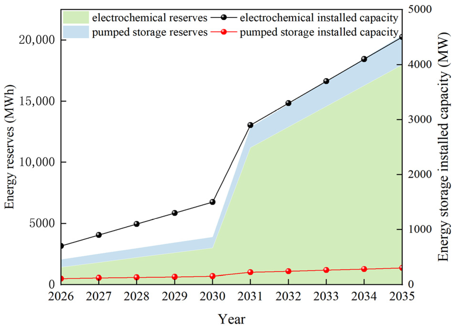
This study models the development of two primary long-duration electricity storage technologies: Pumped Hydro Storage and Battery Energy Storage Systems, with electricity as the stored energy carrier. The projected growth is illustrated in Figure 7. This projection is grounded in regional and national energy strategies aimed at achieving the ‘Dual Carbon’ goals, with targets derived from policy documents such as China’s “14th Five-Year Plan for New Energy Storage Development” [47]. The model assumes that the initial installed capacity in 2025 aligns with policy targets, with PHS at 100 MW/600 MWh. In the future scenario, electrochemical and pumped storage are both growing, with pumped storage increasing at a relatively flat rate. The increase in electrochemical energy storage expands significantly in 2030. In the future scenario, both electrochemical storage and pumped storage show a growth trend, with pumped storage increasing at a relatively flat rate.

5.3. Cost Projections

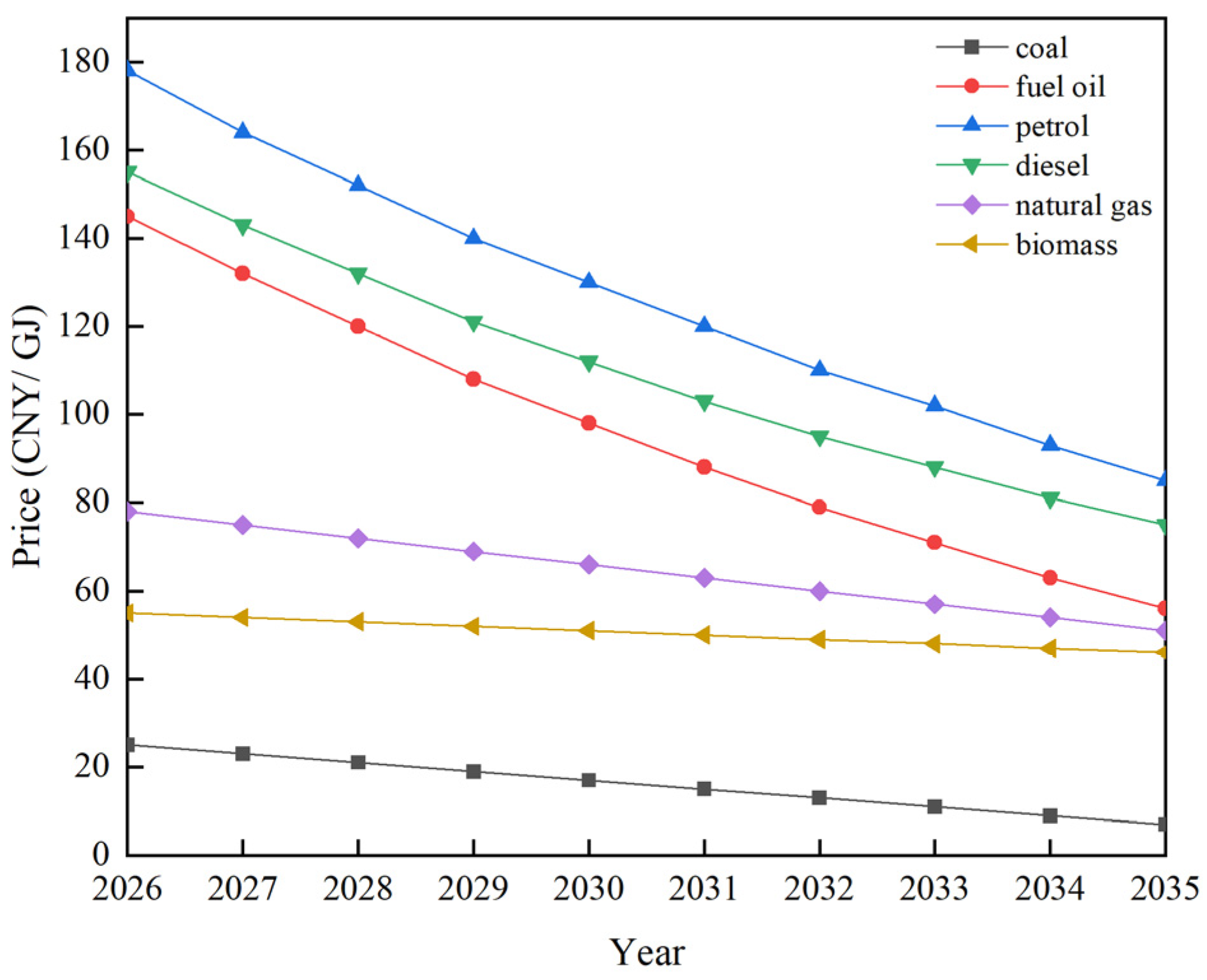
The variable costs of integrated energy systems are highly sensitive to fuel prices. Predicting future fossil fuel prices is inherently complex, as it is influenced by conflicting factors. In a future aligned with deep decarbonization goals, factors such as the large-scale deployment of renewable energy, significant improvements in energy efficiency, and robust climate policies aimed at reducing demand for carbon-intensive fuels are expected to suppress long-term fossil fuel prices. This study analyzes decarbonization pathways, which implicitly assume a future where strong and effective climate policies are implemented. Therefore, in the cost analysis, we adopt a policy-driven price scenario aligned with long-term climate goals, referencing predictions from authoritative institutions such as the IEA in its “Net Zero Emissions by 2050” scenario [48,49,50,51]. This scenario is a globally recognized and technically robust benchmark for modeling ambitious climate mitigation. It is not a simple extrapolation but is based on a comprehensive analysis of global energy markets under a paradigm shift toward clean energy. Its projection of declining fossil fuel demand and subsequently lower prices is a logical outcome of the modeled decarbonization efforts. The price trends adopted are shown in Figure 8.
The economic parameters of the main equipment are shown in Table 4. These parameters, including initial investment and fixed O&M costs, were compiled from a comprehensive review of recent industry reports, scholarly literature, and official policy documents to ensure they reflect China’s current and near-future economic landscape [52,53,54]. The selected investment costs for wind and photovoltaic power provide a conservative baseline for long-term modeling, accounting for potential fluctuations in supply chains and raw material prices. In contrast, thermal power technologies such as coal and gas have more complex system configurations, leading to higher O&M costs. Specifically, the higher investment cost for coal-fired power accounts for the deployment of high-efficiency, ultra-low emission technologies and carbon capture readiness, aligning with national deep decarbonization goals. These carefully chosen parameters establish a robust foundation for calculating total annual system costs and evaluating the economic viability of different decarbonization pathways.

6. Results

6.1. Analysis of Hydrogen Decarbonization Pathway Simulation Results

6.1.1. Analysis of the Evolution of the Energy Structure

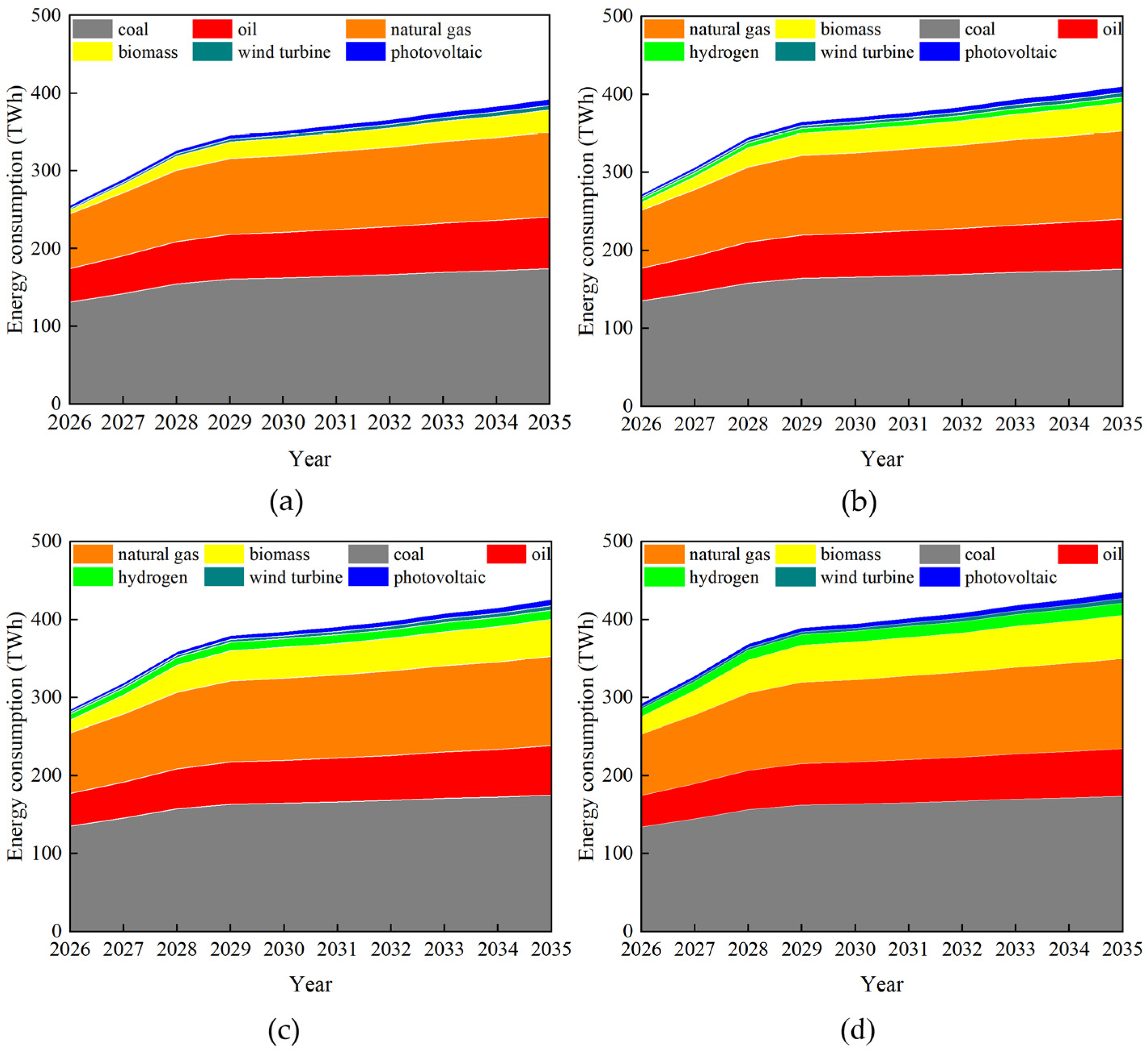
The evolutionary trend of end-use energy supply for each scenario of the integrated energy system in Jinan City is shown in Figure 9. The share of hydrogen energy in end-use fuel consumption in each sector gradually increases with the increase of hydrogen energy penetration in different scenarios. However, the proportion of hydrogen energy consumption in total energy consumption is small, reflecting the current cost and infrastructure challenges of hydrogen technology, but it shows some value in improving power system flexibility, promoting renewable energy utilization, and reducing carbon emissions, foreshadowing the potential growth of hydrogen technology in the future energy system.
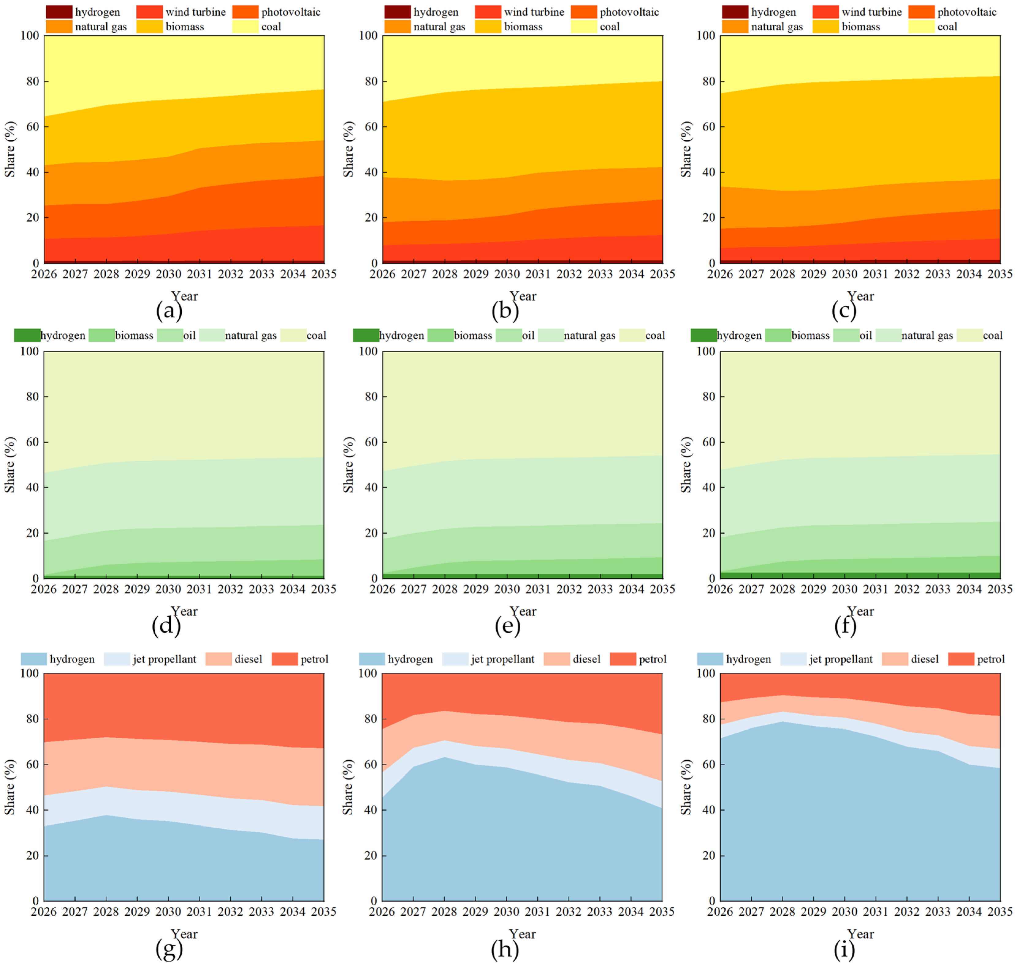
The energy consumption structure of the integrated energy system is divided into three major sectors, namely transportation, industry, and electricity, and the simulation results of the evolutionary trend of primary energy supply in each sector from 2026 to 2035 are shown in Figure 10. The simulation results show that the share of hydrogen fuel in the energy consumption of the transportation sector has increased significantly, and the energy consumption of the transportation sector is dominated by gasoline and diesel in the CRPS scenario, with a low penetration rate of hydrogen fuel. By contrast, the total energy consumption in the transportation sector is projected to decrease significantly in the CHAPS scenario because of the special emphasis placed on the core value of hydrogen fuel in promoting the development of sustainable transportation. This indicates that hydrogen fuel technology and related infrastructure development is crucial to achieving the energy transition and the goal of sustainable development in the transportation sector.
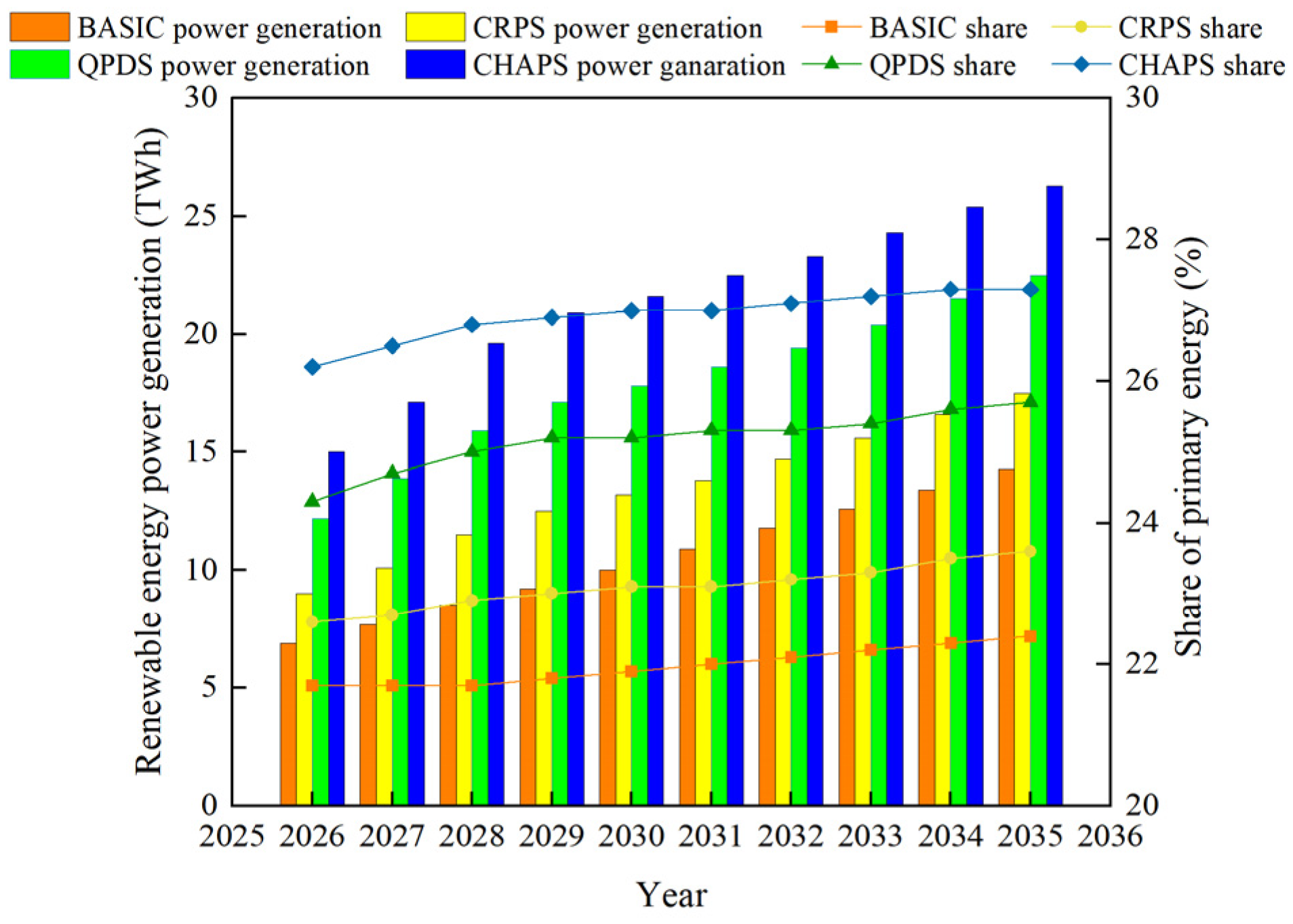
Figure 11 shows the amount and share of renewable energy generation under the different scenarios. With the increase of the installed capacity of wind power, PV, and biomass, the renewable energy generation in all scenarios shows an increasing trend year by year. The increase of renewable energy generation is more obvious in the QPDS scenario, and the CHAPS scenario shows the highest energy share, with 89.9% and 4.9% increases in the renewable energy generation and primary energy share in 2035, respectively. This change reflects the fact that as hydrogen penetration increases, the installed capacity of the electrolyzer increases and the system is able to consume more power.
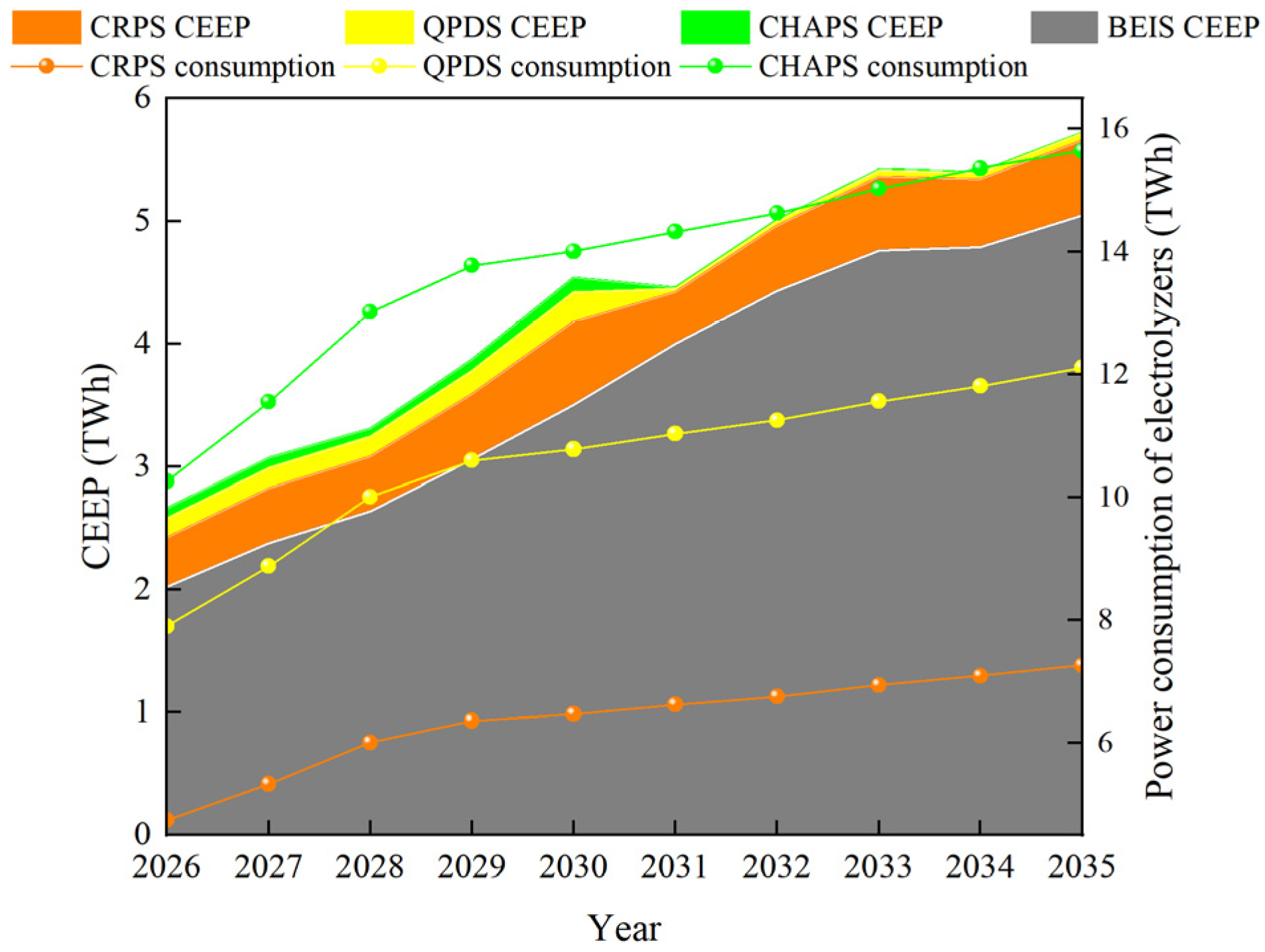
The critical excess electricity versus electrolyzer use for each scenario is shown in Figure 12. In the BEIS scenario, as the installed capacity of renewable energy sources rises, it is difficult for the integrated energy system to fully consume their power generation, resulting in a high share of CEEP. In the hydrogen energy application scenario, the CEEP decreases significantly due to the commissioning of the electrolyzer. In the CRPS, QPDS, and CHAPS scenarios, the higher the penetration of hydrogen in the terminal energy, the lower the CEEP, indicating that the rational allocation of the electrolyzer is significant in enhancing the stability of the integrated energy system.

6.1.2. Carbon Emission Analysis

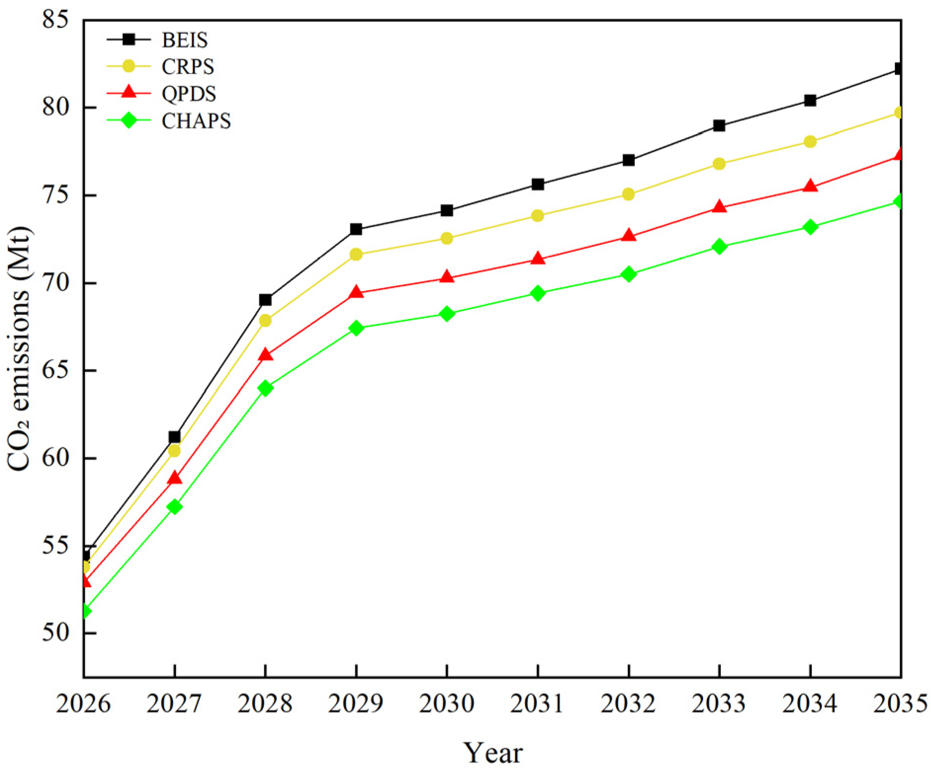
The trend of CO2 emissions in 2026–3035 under different scenarios is shown in Figure 13. Carbon dioxide emissions increase in all scenarios, and the increase slows down until 2029. Compared with the BEIS in 2030, the carbon emission reduction levels of the CRPS scenario, the QPDS scenario, and the CHAPS scenario reach 3.48%, 6.72%, and 10.08%, respectively, which indicates that with the increase of hydrogen penetration and CCS, carbon dioxide emissions can be effectively reduced.
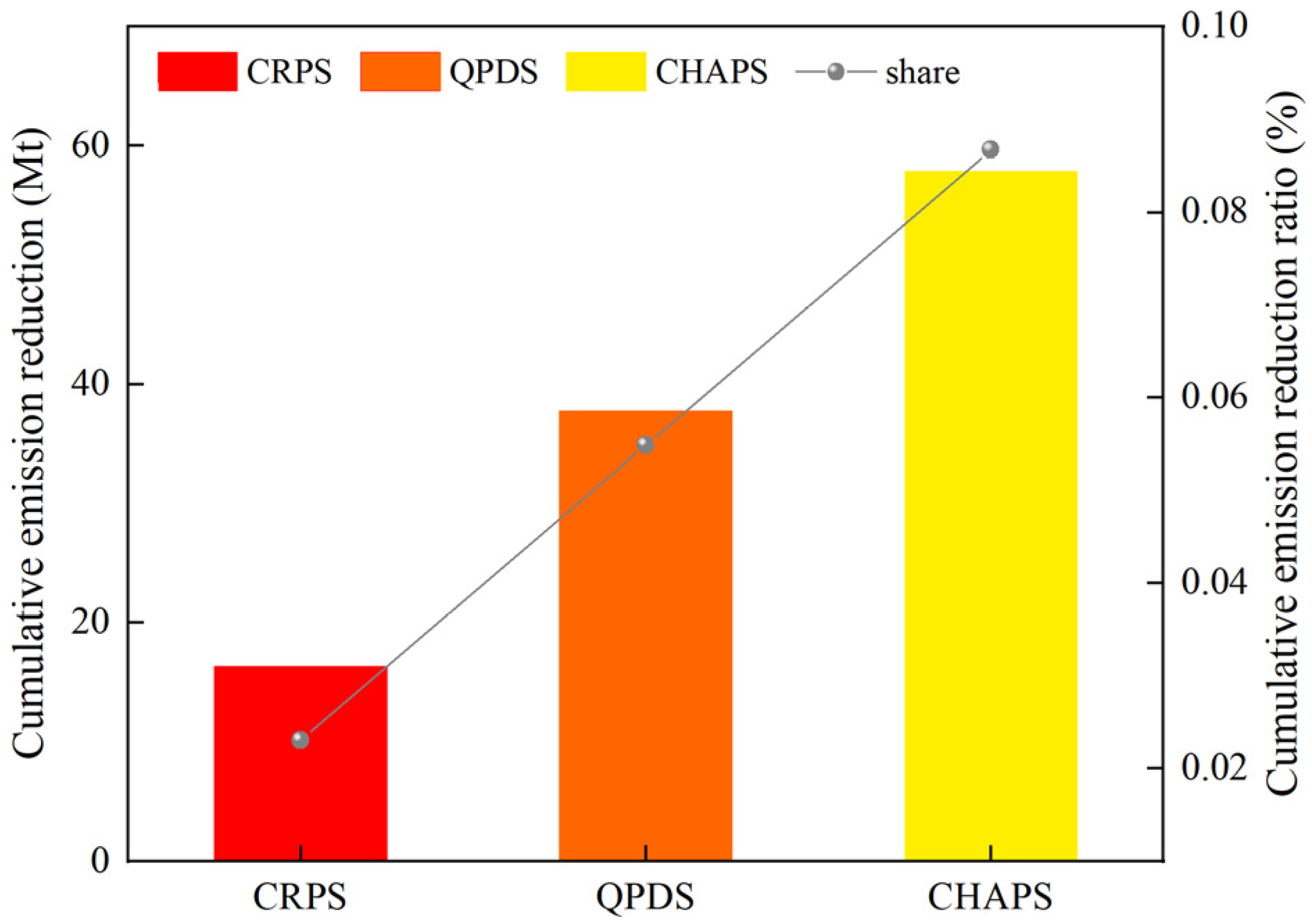
The cumulative carbon dioxide emission reductions and percentages of different scenarios are shown in Figure 14. With the increase of hydrogen energy penetration, the cumulative carbon dioxide emission reduction and the proportion of emissions reduction of each hydrogen energy scenario show an increasing trend, among which the cumulative carbon emissions reduction of the CRPS, QPDS, and CHAPS scenarios reaches 16.34 Mt, 37.74 Mt, and 57.93 Mt, respectively, and the proportion of cumulative carbon emission reduction is 2.30%, 5.48%, and 8.67%, respectively.

6.1.3. System Cost Analysis

Figure 15 shows a comparison of annual costs under different scenarios and quantitatively analyzes the evolution of annual costs over time. As the penetration rate of hydrogen energy in terminal energy increases, the annual costs of the CRPS, QPDS, and CHAPS scenarios gradually rise, and they are all higher than those of the BASIC scenario. The application of hydrogen production and coal-to-hydrogen with CCS technology is the main reason for the cost increase. Given that the proportion of coal, oil, and other fossil energy sources in future energy applications will gradually decline, and the cost of fuel consumption will be reduced accordingly, the annual cost of each scenario will show a decreasing trend after 2029.
To more accurately compare these cost discrepancies, we calculated the RMSE of each hydrogen scenario relative to the BEIS scenario, as shown in Table 5. The RMSE values for the CRPS scenario, QPDS scenario, and CHAPS scenario are 30.57 billion CNY, 53.40 billion CNY, and 67.09 billion CNY, respectively. These values quantify the growing cost gap as hydrogen penetration deepens.
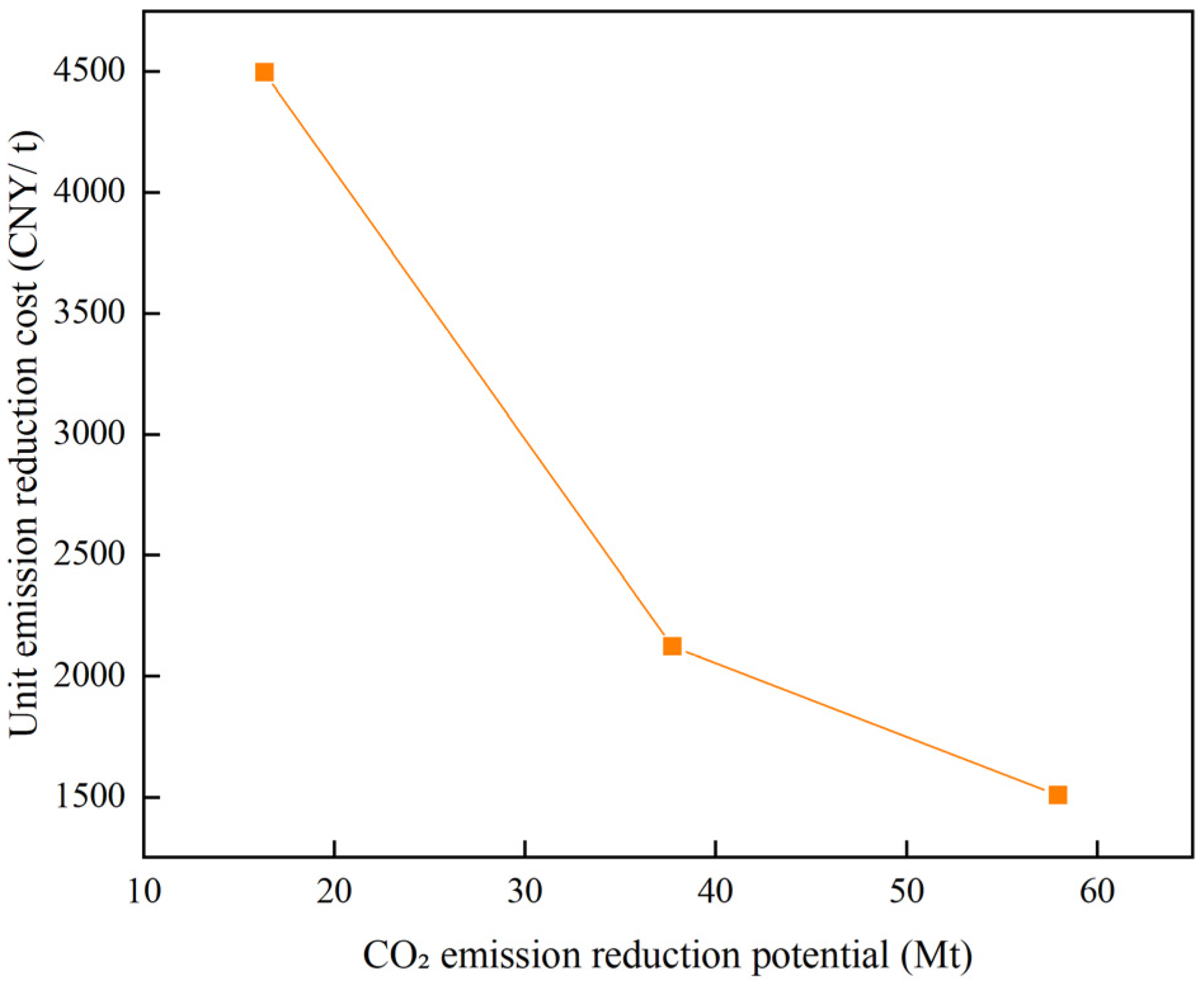
Figure 16 shows the CO2 abatement potential and unit abatement cost of the three hydrogen penetration scenarios compared to the BASIC scenario. The CHAPS scenario shows the lowest unit abatement cost and the highest carbon abatement potential, with reductions of 29.39% and 7.98%, respectively, which demonstrates the excellent abatement performance of its integrated energy system.

6.2. Evaluation of Hydrogen Decarbonization Pathway Simulation Results

The entropy weight method and TOPSIS methods were used to comprehensively evaluate the three different hydrogen energy scenarios of the integrated energy system, using cumulative cost, cumulative carbon emissions, cumulative CEEP, and cumulative renewable power generation as the evaluation indexes. The data of the simulation results of the hydrogen decarbonization pathway are shown in Table 6.
The weight distribution of the indicators is shown in Table 7. The weight distribution of each evaluation index is relatively balanced. Among them, the weight of cumulative cost is the highest, reaching 0.2814, which reflects the relative fairness of the decision-making process and the moderate focus on economic cost factors in the planning and operation of the integrated energy system, taking into account the multiple objectives of the environment, energy efficiency, and the optimization of the energy structure, which helps to achieve the sustainable development of the system on the basis of balancing the needs of all parties.
The simulation results of hydrogen decarbonization pathways under different scenarios are shown in Table 8, in which the CHAPS scenario ranks first with a score of 0.5961, which indicates that this scenario is the closest to the ideal state after considering all the indicators. The QPDS scenario has the lowest score of 0.3154, which indicates that the penetration rate of hydrogen in end-use energy is not as high as possible, but rather, it is necessary to select appropriate hydrogen penetration scenarios in accordance with the actual situation of different energy systems so as to realize the optimal economic, environmental, and sustainabilitybenefits.

6.3. Evaluation of Electricity Supply and Demand Simulation Results

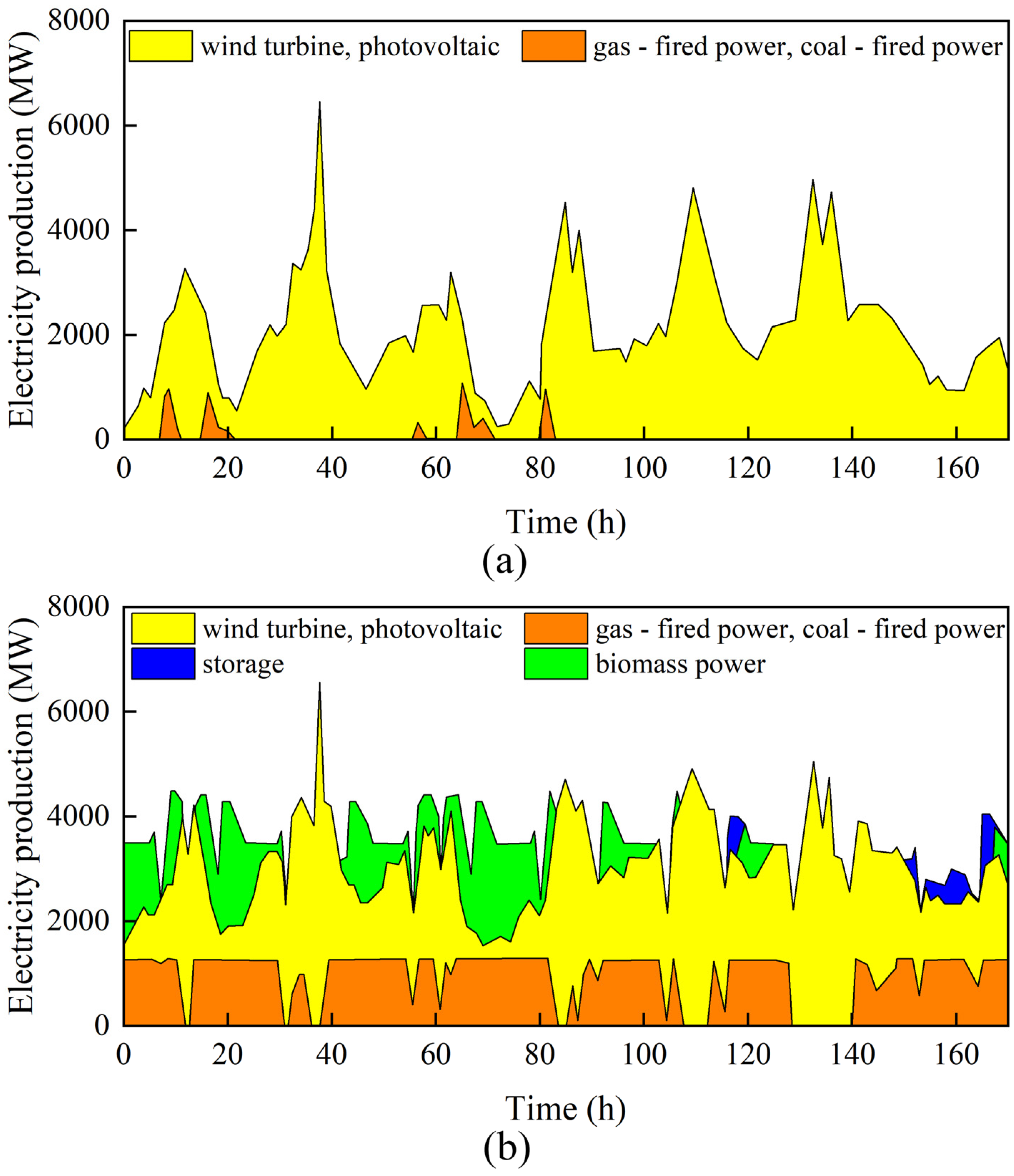
To provide a granular view of the system’s operational dynamics, this section analyzes the electricity supply and demand balance for a representative week in January 2035, comparing the BEIS and CHAPS scenarios. Figure 17 and Figure 18 highlight how hydrogen integration fundamentally alters grid operations.
Figure 17 presents the electricity demand composition. In the BEIS scenario (Figure 17a), the system struggles to absorb all the renewable energy generated. When generation from wind and solar exceeds the final electricity demand and export capacity, the surplus energy is curtailed, resulting in significant CEEP. This represents a substantial waste of clean energy potential. In contrast, the CHAPS scenario (Figure 17b) demonstrates a highly effective solution to this problem. The previously curtailed excess power is now channeled to power electrolyzers for green hydrogen production. This new, flexible demand from the electrolyzer almost entirely eliminates CEEP, effectively converting what would have been wasted energy into a valuable energy carrier, thereby significantly improving the overall system efficiency and renewable energy utilization rate.
Figure 18 presents the electricity supply composition. In the BEIS scenario (Figure 18a), the supply structure is heavily reliant on variable wind and solar, with coal and natural gas plants providing residual balancing and flexibility. This leads to periods of fossil fuel consumption to meet demand when renewable generation is low. The supply structure under the CHAPS scenario (Figure 18b) is markedly different and fully decarbonized. To complement the high penetration of variable renewables, dispatchable biomass power plants are introduced to ensure grid stability and meet residual load, particularly during periods of low wind and solar output. As defined in Section 5.2, biomass is a planned component of the future renewable energy mix. Its role here is crucial for providing the necessary firm capacity to balance the grid in a system without fossil fuels. This, combined with an expanded deployment of electricity storage, creates a resilient and flexible power system that can reliably match supply with the newly expanded demand, ensuring a dynamic balance.

7. Discussion

The study quantitatively analyzes and comprehensively evaluates the decarbonization pathways of urban integrated energy systems under different hydrogen penetration rates by constructing a coupled multisectoral EnergyPLAN model and combining the entropy weight and TOPSIS methods. The results of the study reveal the non-linear relationship between hydrogen penetration rate and comprehensive system benefits, especially the finding that the “Hydrogen Alliance Potential Scenario” is better than the “Policy-Driven Scenario”, which provides an important quantitative reference for cities to formulate hydrogen energy development strategies, challenging the assertion that the higher the hydrogen energy share is, the more the city’s energy system will be able to decarbonize. It challenges the intuitive perception that “the higher the proportion of hydrogen energy, the better”. However, in order to ensure the rigor and completeness of the study, it is necessary to discuss the limitations of this study in depth and to look forward to future research directions.

7.1. Research Limitations

i.
The use of a priori settings for cross-sectoral hydrogen allocation, with fixed hydrogen substitution efficiencies for fossil fuels, reduces hydrogen utilization in the industrial sector to coal substitution and injection into natural gas pipeline networks. Whereas hydrogen substitution efficiencies are closely related to specific application technologies (such as gas turbine hydrogen doping ratios) and are dynamic parameters, the use of fixed values makes it difficult to adequately capture the impact of technical details on system energy efficiency. The industrial sector has been neglected in terms of the use of hydrogen as a chemical feedstock or high-temperature process, which feature significant differences in economics and abatement potential, which in turn may underestimate the role of hydrogen in industrial decarbonization. Ideally, hydrogen allocation should be dynamically optimized based on the marginal abatement cost of each sector, and preset values make it difficult to achieve the global optimum of the system.
ii.
The model’s key technology costs and fossil fuel prices are projected using linear trends, and the selected future data and efficiency parameters are more optimistic. Whereas the cost reductions of hydrogen-related technologies show a non-linear “learning curve” characteristic, static or linear projections may overestimate the long-term costs of hydrogen penetration scenarios. At the same time, international fuel prices and future carbon pricing mechanisms are subject to large uncertainties, and a fixed forecast curve is difficult to make cover the risk of future fluctuations, all of which can affect the accuracy of the model’s economic assessment.
iii.
The core of this study is an EnergyPLAN-based energy flow balance simulation, which focuses on “hydrogen use side analysis”, but the hydrogen energy supply chain and infrastructure modeling is insufficient, and the costing and layout modeling of “hydrogen supply side” infrastructure, i.e., the whole chain of “production–storage–delivery–use”, has not been carried out in detail, and the model lacks a dynamic optimization mechanism for selecting among green, blue, and gray hydrogen sources. There is no detailed costing and layout modeling of the “hydrogen supply side” infrastructure, i.e., the whole chain of “production–storage–delivery–use”, and the existing models only consider hydrogen as a usable fuel input, which may underestimate the overall social costs required to realize each scenario.
iv.
The model analyzes Jinan as a single energy node without considering the spatial heterogeneity within the city, and there are limitations in the spatial resolution of the model, thus ignoring issues such as regional grid transmission bottlenecks, natural gas pipeline network hydrogen doping limitations, and mismatches between the geographic distribution of renewable energy sources, such as photovoltaics, and load centers, etc. In fact, the siting of large-scale electrolytic water-to-hydrogen plants is subject to stringent constraints in terms of grid access capacity and water resource conditions. Such spatial factors can adversely affect the overall layout and operating costs of the system.

7.2. Future Research Perspectives

i.
Future research will construct more refined sub-sector models and develop more refined sub-models for the characteristics of hydrogen use in different sectors. In the transportation sector, dynamic models will be constructed based on the ownership, penetration, and behavioral patterns of different vehicle types (fuel cell vehicles and hydrogen internal combustion engine vehicles). In the industrial sector, different uses of hydrogen as a fuel and raw material will be distinguished and modeled in conjunction with specific industrial processes to more accurately assess hydrogen’s emissions reduction potential and economic value.
ii.
In the future, we will embed dynamic learning curves for key technologies in our model, dynamically depicting how costs change over time and scale of deployment. At the same time, using stochastic planning or multi-scenario analysis to cope with the uncertainties in the external environment, such as fuel prices and carbon prices, to assess the robustness of different decarbonization paths, and ultimately to propose more adaptive strategic recommendations.
iii.
In the future, the existing energy system model will be deeply integrated with the geographic information system to carry out spatial and temporal optimization studies for the whole chain of hydrogen energy “production–storage–transmission–use”, and optimize the siting and scale of hydrogen production facilities, storage, and refueling stations, taking into account the endowment of renewable energy resources, water resources distribution, constraints of power grids and pipeline networks, land use, and safety distances. Thus, we will form a blueprint for the development of hydrogen energy infrastructure that is spatially feasible and economically reasonable.
iv.
Extend the research scope from technical and economic analysis to socio-economic areas, explore the effectiveness of subsidy policies, carbon trading mechanisms, and a hydrogen certificate system on the development of hydrogen energy, assess the pulling effect of the hydrogen industry on local employment and economic growth, and analyze the public’s acceptance of hydrogen energy infrastructure through questionnaire surveys, in order to provide more comprehensive support to policy formulation, a more accurate portrayal of the role of hydrogen energy in the urban energy transition, and guidance for the scientific operation of the path to achieve the “dual carbon” goal.

8. Conclusions

Based on the EnergyPLAN model to construct an integrated energy system coupled with electric power, transportation, and industrial sectors, four hydrogen energy penetration scenarios were set up with Jinan City as the research object. The entropy weight method and TOPSIS method were combined to evaluate the dimensions of cost, carbon emission, and sustainability and to explore the impact of hydrogen energy penetration rate changes on the decarbonization path of the urban integrated energy system. The main conclusions are as follows. Our work’s novelty stems from overcoming the limitations of common single-sector analyses by innovatively quantifying the effects of graduated hydrogen penetration, as opposed to a simple with/without comparison. This granular method reveals complex, non-linear trade-offs and synergies across end-use sectors, leading to a more realistic and actionable assessment for urban energy planning.
i.
The Hydrogen Alliance Potential Scenario has the best performance in decarbonization, with CO2 emission reduction potential and unit emission reduction cost improve by 7.98% and 29.39%, respectively, and renewable energy power generation and primary energy share increased by 89.9% and 4.9% in 2035 compared with the baseline energy inertia scenario, showing the strongest carbon emission reduction capability and renewable energy consumption potential.
ii.
The comprehensive evaluation results show that the Hydrogen Alliance Potential Scenario ranks first with a relative closeness of 0.5961, which is closest to the ideal state in terms of the balance of cost, environment, and sustainability indicators. The Policy-Driven Scenario has the lowest score (0.3154), which indicates that hydrogen penetration is not “the higher the better” and that the selection of an appropriate solution needs to be combined with the actual needs of the system.
iii.
Hydrogen penetration has a positive effect on the optimization of the energy structure. As the share of hydrogen in end-fuel consumption increases in all scenarios, the expansion of the installed capacity of electrolysis tanks effectively reduces the critical excess power and improves the stability of the system. However, the current proportion of hydrogen in the total energy consumption is still low, reflecting that the cost of the technology and the construction of the infrastructure are still the main constraints.
iv.
In terms of system costs, the annual costs of the hydrogen-containing scenarios are all higher than those of the baseline energy inertia scenario, mainly due to the inputs of hydrogen production and coal-to-hydrogen with CCS technology. However, the costs of the scenarios take on a downward trend after 2029, which predicts that with the decrease in the proportion of fossil energy sources, the economics of the hydrogen energy system will gradually improve.

Author Contributions

Conceptualization, H.W.; Data curation, Y.L.; Formal analysis, H.W. and X.Z.; Funding acquisition, J.L.; Investigation, H.W., Y.L., X.Z., B.G. and J.L.; Methodology, H.W. and J.L.; Project administration, B.G. and J.L.; Software, X.Z., Y.L. and X.Z.; Supervision, J.L.; Visualization, H.W.; Writing—original draft, H.W.; Writing—review and editing, H.W., Y.L., X.Z., B.G. and J.L. All authors have read and agreed to the published version of the manuscript.

Funding

This work was funded by the Chengdu Technology Innovation R&D Project (2024-YF05-00682-SN) and Sichuan Huashi Group Technology Project (HXKX2024/004).

Data Availability Statement

Data is contained within the article.

Acknowledgments

This work was also supported by the Plan of Introduction and Cultivation for Young Innovative Talents in Colleges and Universities of Shandong Province.

Conflicts of Interest

Author Dr. Bo Gao was employed by Sichuan Institute of Building Research. The remaining authors declare that the research was conducted in the absence of any commercial or financial relationships that could be construed as a potential conflict of interest.

Appendix A

Appendix A.1. Data Sources and Variable Descriptions

The historical data used for regression analysis in this study was obtained from the Jinan City Statistical Yearbook. The variables were the terminal energy consumption of various sectors, and the independent variables included per capita GDP, population size, the proportion of secondary industries, urbanization rate, and consumer price index.

Appendix A.2. Regression Analysis Methods

This study used a multiple linear regression model and IBM SPSS Statistics 27 for variable screening. This method automatically introduces or removes variables based on their contribution to the model, ultimately retaining the most statistically significant combination of variables. The model screening method is shown below:
i.
Perform significance tests on the model by first conducting t-statistic on each regression coefficient to calculate their significance p-values. Typically, the significance level α = 0.05. If p > 0.05, it is concluded that the independent variable has no significant effect on the dependent variable and should be removed from the model.
ii.
The F statistic reflects the extent to which all independent variables in the model collectively explain the variation in the dependent variable. The larger the F statistic, the more significant the linear relationship in the model. If the significance of the F-test < 0.05, it indicates that the regression model is statistically significant and meaningful overall.
iii.
Next, the goodness of fit of the model is assessed using the adjusted R2 to evaluate the model’s overall explanatory power. A higher adjusted R2 indicates better model fit to the data.

Appendix A.3. Regression Analysis Methods

Appendix A.3.1. Regression Results of the Electricity Demand Model

The results of the regression analysis of electricity demand are shown in Table A1 and Table A2. The population variable in the initial model was excluded because its p-value was 0.171 (>0.05), which was not statistically significant.
Table A1. Final model regression coefficient table for the electricity sector.
VariableCoefficient of RegressionStandard Errort-Statisticp-Value
lnDEl24.0029.6202.4950.014
lnGDP0.1930.0862.2440.027
lnSec1.3780.4922.8010.006
lnUrb8.7830.43320.284<0.001
lnEte−3.5861.379−2.6000.011
Table A2. Summary of the final model fit for the electricity sector.
IndicatorNumerical Value
R20.988
Adjusted R20.986
F statistic578.377
Significance of F-test<0.001
Note: Significance level α = 0.05

Appendix A.3.2. Regression Analysis Results of the Industrial Sector Energy Demand Forecast Model

The results of the regression analysis of energy demand in the industrial sector are shown in Table A3 and Table A4. In the initial model, the population variable was excluded because its p-value was 0.284 (>0.05) and was therefore not statistically significant.
Table A3. Final model regression coefficient table for the industrial sector.
VariableCoefficient of RegressionStandard Errort-Statisticp-Value
lnDIn−14.0013.931−3.5620.002
lnGDP0.7330.06611.106<0.001
lnSec1.0930.3692.9620.004
lnUrb−0.340.141−2.4110.025
lnEte4.020.9054.442<0.001
Table A4. Summary of the final model fit for the industrial sector.
IndicatorNumerical Value
R20.982
Adjusted R20.980
F statistic460.89
Significance of F-test<0.001
Note: Significance level α = 0.05

Appendix A.3.3. Regression Analysis Results of the Transportation Sector Energy Demand Forecast Model

The results of the regression analysis of energy demand in the transportation sector are shown in Table A5 and Table A6. In the initial model, the population variable was excluded because its p-value was 0.381 (>0.05), which was not statistically significant.
Table A5. Final model regression coefficient table for the transportation sector.
VariableCoefficient of RegressionStandard Errort-Statisticp-Value
lnDET−23.0717.967−2.8960.005
lnGDP1.2540.1339.429<0.001
lnSec1.3540.6132.2100.032
lnUrb−1.9970.287−6.966<0.001
lnEte4.7631.8352.5960.023
Table A6. Summary of the final model fit for the transportation sector.
IndicatorNumerical Value
R20.985
Adjusted R20.982
F statistic256.708
Significance of F-test<0.001
Note: Significance level α = 0.05

References

  1. Pu, Z.; Yi, T. Low-carbon economic energy sharing and revenue distribution strategy for multi-integrated energy systems considering the uncertainty of new energy output. Sustain. Energy Grids Netw. 2025, 43, 101757. [Google Scholar] [CrossRef]
  2. Wang, Y.; Zhou, H.; Ma, K.; Jiang, S.; Zhu, M. Dynamic pricing and low-carbon economy dispatch of multi-park integrated energy system based on mixed game. Electr. Power Syst. Res. 2025, 248, 111908. [Google Scholar] [CrossRef]
  3. Cordioli, E.; Maigret, J.d.; Testi, M.; Crema, L. Green hydrogen in the Alps: Mapping local stakeholders perspectives and identifying opportunities for decarbonization. Energy Rep. 2025, 14, 128–140. [Google Scholar] [CrossRef]
  4. Wang, Z.; Mu, X.; Ma, Y.; Liao, P.; Ji, Y.; Han, F. Advanced energy management and optimal scheduling for integrated offshore gas-hydrogen-electricity-heat systems. Energy 2025, 319, 135091. [Google Scholar] [CrossRef]
  5. Zhang, Z.; Xu, Y.; Yu, Y.; Chen, X.; Liao, H. Stochastic multiple criteria decision-making for configuration selection of electricity-hydrogen integrated energy systems with multiple stakeholder interest coordination. Eng. Appl. Artif. Intell. 2025, 157, 111323. [Google Scholar] [CrossRef]
  6. Wade, F.; Roche, R.; Chailan, A.; Bertrand, V.; Paire, D. Optimal sizing and energy management of an integrated energy system coupling a hydrogen-fueled gas turbine with storage for Power-to-Power and hydrogen supply. Int. J. Hydrogen Energy 2025, 135, 31–47. [Google Scholar] [CrossRef]
  7. Wu, K.; Jiang, M.; Huang, Y.; Dai, Z.; Wang, X.; Duan, Z.; Wang, Y.; Li, G. Optimization of multi-objective capacity allocation and performance analysis for integrated energy systems considering hydrogen storage. Energy 2025, 325, 136160. [Google Scholar] [CrossRef]
  8. Xu, X.; Wang, B.; Shi, M.; Li, G.; Zhang, Y.; Wang, Q.; Liu, D. Research on hydrogen storage system configuration and optimization in regional integrated energy systems considering electric-gas-heat-hydrogen integrated demand response. Int. J. Hydrogen Energy 2025, 135, 86–103. [Google Scholar] [CrossRef]
  9. Yang, S.; Yan, R.; Zhang, J.; Wang, J.; Bai, Z.; He, Y.; Hu, K.; Ao, X. Nested long-short-term temporal compression optimization for high-renewable integrated energy systems with hydrogen storage and heat recovery. Energy 2025, 333, 137423. [Google Scholar] [CrossRef]
  10. Wu, T.; Wang, J.; Zhao, T. Coordinated planning of integrated energy system with hydrogen hub. Appl. Energy 2025, 394, 126089. [Google Scholar] [CrossRef]
  11. Li, X.; Du, Y.; Tan, Z.; He, H.; Fan, W. Optimal operation model of electrothermal integrated energy system including hydrogen production from offshore wind power participating in multi-level market. Int. J. Hydrogen Energy 2025, 114, 250–266. [Google Scholar] [CrossRef]
  12. Lu, S.; Cui, M.; Gao, B.; Liu, J.; Ni, J.; Liu, J.; Zhou, S. A Comparative Analysis of Machine Learning Algorithms in Predicting the Performance of a Combined Radiant Floor and Fan Coil Cooling System. Buildings 2024, 14, 1659. [Google Scholar] [CrossRef]
  13. Ding, Y.; Lu, S.; Li, T.; Zhu, Y.; Wei, S.; Tian, Z. An indoor thermal environment control model based on multimodal perception and reinforcement learning. Build. Environ. 2025, 276, 112863. [Google Scholar] [CrossRef]
  14. Lu, S.; Zhou, S.; Ding, Y.; Kim, M.K.; Yang, B.; Tian, Z.; Liu, J. Exploring the comprehensive integration of artificial intelligence in optimizing HVAC system operations: A review and future outlook. Results Eng. 2025, 25, 103765. [Google Scholar] [CrossRef]
  15. Dong, X.; Zhao, Y. An economic way to reduce emissions of industrial parks with hydrogen-based integrated energy systems. Int. J. Hydrogen Energy 2025, 106, 1122–1133. [Google Scholar] [CrossRef]
  16. Wang, Y.; Qin, Y.; Ma, Z.; Wang, Y.; Li, Y. Operation optimisation of integrated energy systems based on cooperative game with hydrogen energy storage systems. Int. J. Hydrogen Energy 2023, 48, 37335–37354. [Google Scholar] [CrossRef]
  17. Yang, Z.; Cheng, L.; Min, H.; Lei, Y.; Yang, Y. Distributionally robust optimization-based scheduling for a hydrogen-coupled integrated energy system considering carbon trading and demand response. Glob. Energy Interconnect. 2025, 8, 175–187. [Google Scholar] [CrossRef]
  18. Zhan, Z.; Xu, J.; Zhang, T.; Kong, X.; Li, H.; Zhang, B. Optimal scheduling of integrated wind- photovoltaic-hydrogen energy system considering hydrogen application and waste heat recovery. Energy Rep. 2024, 11, 3684–3694. [Google Scholar] [CrossRef]
  19. Sohani, A. Time-dependent energy, economic, and environmental assessment of a PV-hydrogen integrated power system. Int. J. Hydrogen Energy 2025, 144, 964–976. [Google Scholar] [CrossRef]
  20. Liu, X.; Zu, L.; Wei, Z.; Wang, Y.; Pan, Z.; Xiao, G.; Jenkins, N. Two-layer optimal scheduling of integrated electric-hydrogen energy system with seasonal energy storage. Int. J. Hydrogen Energy 2024, 82, 1131–1145. [Google Scholar] [CrossRef]
  21. Fang, X.; Dong, W.; Wang, Y.; Yang, Q. Multi-stage and multi-timescale optimal energy management for hydrogen-based integrated energy systems. Energy 2024, 286, 129576. [Google Scholar] [CrossRef]
  22. Judge, M.A.; Franzitta, V.; Curto, D.; Marvuglia, A. Cost-effective optimization of energy system integrated with hybrid battery-hydrogen storage: A techno-economic and environmental analysis for the sustainable electrification of a university campus. J. Energy Storage 2025, 130, 117133. [Google Scholar] [CrossRef]
  23. Joseph, A.; Allahham, A.; Walker, S.L. Investment decisions in a liberalised energy market with generation and hydrogen-based vector coupling storage in Integrated Energy System: A game-theoretic model-based approach. Int. J. Electr. Power Energy Syst. 2025, 166, 110518. [Google Scholar] [CrossRef]
  24. Li, J.; Chen, H.; Qi, Y.; Wang, Y.; Lei, J. Collaborative optimization for cross-regional integrated energy systems producing electricity-heat-hydrogen based on generalized Nash bargaining. Energy 2025, 333, 137444. [Google Scholar] [CrossRef]
  25. Lund, H.; Thellufsen, J.Z.; Østergaard, P.A.; Sorknæs, P.; Skov, I.R.; Mathiesen, B.V. EnergyPLAN–Advanced analysis of smart energy systems. Smart Energy 2021, 1, 100007. [Google Scholar] [CrossRef]
  26. Amil, C.; Yılmazoğlu, M.Z. The importance of hydrogen for energy diversity of Turkey’s energy production: 2030 projection. Int. J. Hydrogen Energy 2022, 47, 19935–19946. [Google Scholar] [CrossRef]
  27. Koivunen, T.; Khosravi, A.; Syri, S. The role of power–to–hydrogen in carbon neutral energy and industrial systems: Case Finland. Energy 2023, 284, 128624. [Google Scholar] [CrossRef]
  28. Maaouane, M.; Zouggar, S.; Krajačić, G.; Zahboune, H. Modelling industry energy demand using multiple linear regression analysis based on consumed quantity of goods. Energy 2021, 225, 120270. [Google Scholar] [CrossRef]
  29. Nicoară-Farcău, O.; Wang, X.; Luo, X. Definition of SPSS: We need to speak the same language. J. Hepatol. 2020, 73, 463–464. [Google Scholar] [CrossRef]
  30. Wang, X.; Cheng, T.; Hong, H.; Guo, H.; Lin, X.; Yang, X.; Nie, B.; Hu, Z.; Zou, J. Challenges and opportunities in hydrogen storage and transportation: A comprehensive review. Renew. Sustain. Energy Rev. 2025, 219, 115881. [Google Scholar] [CrossRef]
  31. Ali, N.; Tormene, F. An innovative method for blending hydrogen into natural gas. Int. J. Hydrogen Energy 2025, 148, 150038. [Google Scholar] [CrossRef]
  32. IEA. Net Zero by 2050. 2021. Available online: https://www.iea.org/reports/net-zero-by-2050 (accessed on 27 May 2025).
  33. Prina, M.G.; Dallapiccola, M.; Moser, D.; Sparber, W. Machine learning as a surrogate model for EnergyPLAN: Speeding up energy system optimization at the country level. Energy 2024, 307, 132735. [Google Scholar] [CrossRef]
  34. Villasante, A.; Fernández-Serrano, Á.; Osuna-Sequera, C.; Hermoso, E. Methodology for stiffness prediction in structural timber using cross-validation RMSE analysis. J. Build. Eng. 2025, 107, 112767. [Google Scholar] [CrossRef]
  35. Bamisile, O.; Wang, X.; Adun, H.; Joseph Ejiyi, C.; Obiora, S.; Huang, Q.; Hu, W. A 2030 and 2050 feasible/sustainable decarbonization perusal for China’s Sichuan Province: A deep carbon neutrality analysis and EnergyPLAN. Energy Convers. Manag. 2022, 261, 115605. [Google Scholar] [CrossRef]
  36. IEA. Global Energy Review 2025. 2025. Available online: https://www.iea.org/reports/global-energy-review-2025 (accessed on 13 June 2025).
  37. Ross-Hopley, D.; Rahman, S.; Ugwu, L.; Ibrahim, H. Techno-economic opportunities for integration of renewable energy into the Saskatchewan energy system using EnergyPLAN. Energy 2025, 318, 134903. [Google Scholar] [CrossRef]
  38. Ouyang, Y.; Shen, Z.; Zuo, Q.; Li, Q.; Ma, Y.; Zhang, H. Investigation of rotary proton exchange membrane fuel cell performance optimization based on orthogonal experiment and entropy weight method. Appl. Therm. Eng. 2025, 272, 126362. [Google Scholar] [CrossRef]
  39. Wang, Y.; Zhong, K.; He, J.; Kang, Y. Numerical study on balancing air quality in streets and adjacent neighborhoods using combined porous media model and TOPSIS method. Build. Environ. 2025, 282, 113219. [Google Scholar] [CrossRef]
  40. Mi, Z.; Yuan, B.; Zhang, J. Study on the Scale of New Energy Development during the 14th Five-Year Plan Period. IOP Conf. Ser. Earth Environ. Sci. 2019, 371, 042059. [Google Scholar] [CrossRef]
  41. Su, Y.; Liu, H.; Su, H.; Sun, L. Coupling analysis of land space development and protection and economic and social development in Julu County. IOP Conf. Ser. Earth Environ. Sci. 2020, 602, 012014. [Google Scholar] [CrossRef]
  42. Wang, C.; Cao, Y. Forecasting Chinese economic growth, energy consumption, and urbanization using two novel grey multivariable forecasting models. J. Clean. Prod. 2021, 299, 126863. [Google Scholar] [CrossRef]
  43. Liu, Z.; Huang, X.; Qi, X. Economic effect of China’s carbon neutrality target under shared socioeconomic pathways. Sci. China Earth Sci. 2025, 68, 142–157. [Google Scholar] [CrossRef]
  44. Mallapaty, S. How China could be carbon neutral by mid-century. Nature 2020, 586, 482–483. [Google Scholar] [CrossRef] [PubMed]
  45. Dai, J.; Yang, X.; Wen, L. Development of wind power industry in China: A comprehensive assessment. Renew. Sustain. Energy Rev. 2018, 97, 156–164. [Google Scholar] [CrossRef]
  46. Franke, K.; Garcia, J.F.; Kleinschmitt, C.; Sensfuß, F. Assessing worldwide future potentials of renewable electricity generation: Installable capacity, full load hours and costs. Renew. Energy 2024, 226, 120376. [Google Scholar] [CrossRef]
  47. Wang, X.; Teng, F.; Yang, X.; Wei, R. Assessing the Role of Electricity Storage in China’s High Renewable Energy Penetration Future. Energy Procedia 2017, 105, 4084–4089. [Google Scholar] [CrossRef]
  48. Chepeliev, M.; van der Mensbrugghe, D. Global fossil-fuel subsidy reform and Paris Agreement. Energy Econ. 2020, 85, 104598. [Google Scholar] [CrossRef]
  49. Li, S.; Kong, W.; Wang, Y.; Yuan, L. Medium and long-term energy demand forecasts by sectors in China under the goal of “carbon peaking & carbon neutrality”: Based on the LEAP-China model. Energy 2024, 310, 133017. [Google Scholar]
  50. Mercure, J.F.; Pollitt, H.; Viñuales, J.E.; Edwards, N.R.; Holden, P.B.; Chewpreecha, U.; Salas, P.; Sognnaes, I.; Lam, A.; Knobloch, F. Macroeconomic impact of stranded fossil fuel assets. Nat. Clim. Change 2018, 8, 588–593. [Google Scholar] [CrossRef]
  51. Gugler, K.; Haxhimusa, A.; Liebensteiner, M. Carbon pricing and emissions: Causal effects of Britain’s carbon tax. Energy Econ. 2023, 121, 106655. [Google Scholar] [CrossRef]
  52. Zhang, M.; Cong, N.; Song, Y.; Xia, Q. Cost analysis of onshore wind power in China based on learning curve. Energy 2024, 291, 130459. [Google Scholar] [CrossRef]
  53. Zhao, C.; Zhang, W.; Wang, Y.; Liu, Q.; Guo, J.; Xiong, M.; Yuan, J. The economics of coal power generation in China. Energy Policy 2017, 105, 1–9. [Google Scholar] [CrossRef]
  54. Saravanan, A.; Yaashikaa, P.R.; Kumar, P.S.; Thamarai, P.; Deivayanai, V.C.; Rangasamy, G. A comprehensive review on techno-economic analysis of biomass valorization and conversional technologies of lignocellulosic residues. Ind. Crops Prod. 2023, 200, 116822. [Google Scholar] [CrossRef]
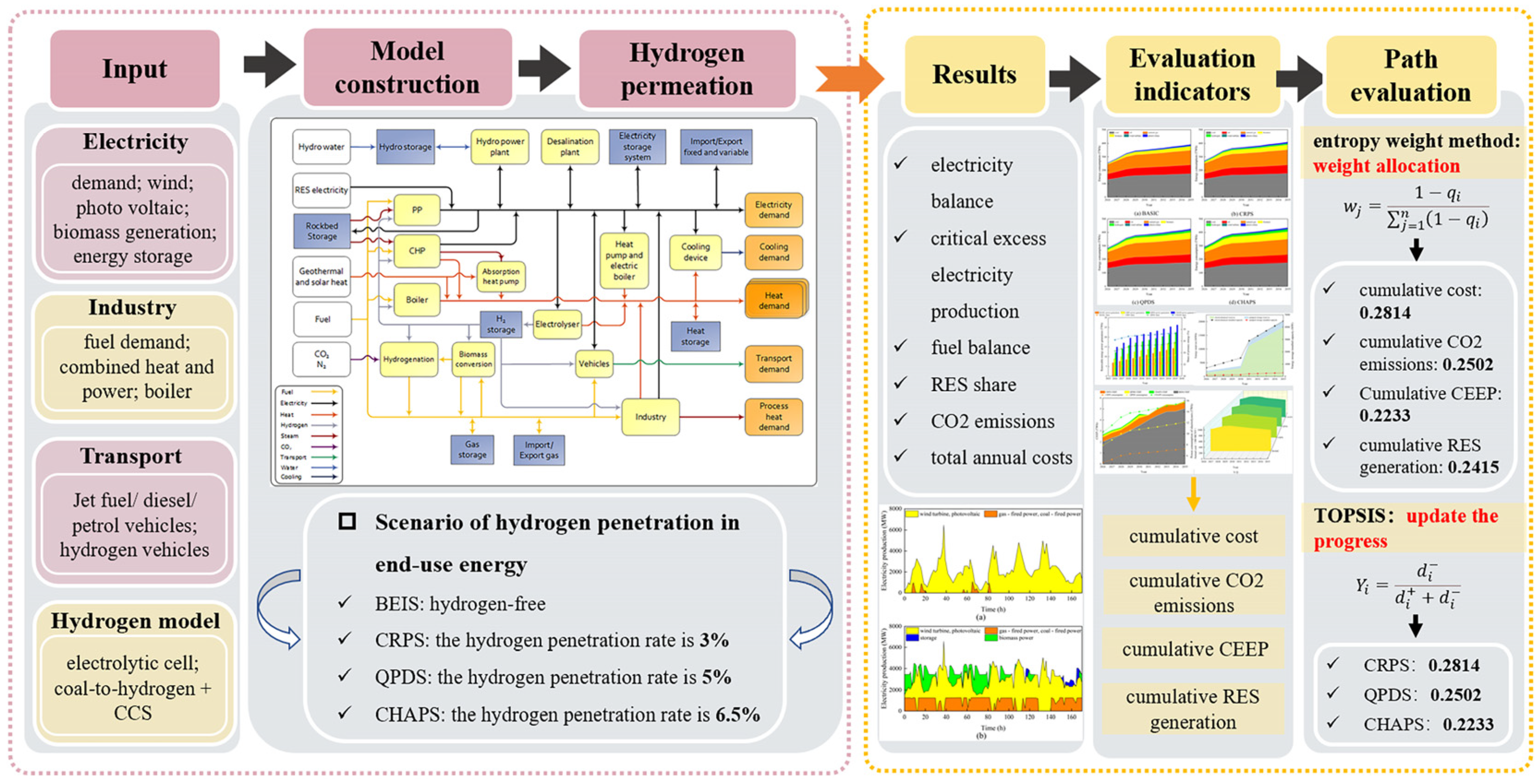
Figure 1. Model architecture for hydrogen application in integrated energy systems.
Buildings 15 03014 g001
Figure 2. Proportion of demand distribution in hydrogen energy application scenarios: (a) distribution of hydrogen demand and (b) distribution of hydrogen supply.
Buildings 15 03014 g002
Figure 3. Forecast of electricity demand over the next 10 years.
Buildings 15 03014 g003
Figure 4. Forecast of industrial fuel demand over the next 10 years.
Buildings 15 03014 g004
Figure 5. Forecast of transportation fuel demand over the next 10 years.
Buildings 15 03014 g005
Figure 6. Prediction of power–installed capacity in the next 10 years.
Buildings 15 03014 g006
Figure 7. Forecast of energy storage installed capacity and storage reserves in the next 10 years.
Buildings 15 03014 g007
Figure 8. Fuel–price forecast for the next 10 years.
Buildings 15 03014 g008
Figure 9. Trends in the evolution of end-use energy supply across scenarios: (a) BASIC, (b) CRPS, (c) QPDS and (d) CHAPS.
Buildings 15 03014 g009
Figure 10. Trends in primary energy evolution in the hydrogen scenario sector: (a) CRPS in electricity, (b) QPDS in electricity, (c) CHAPS in electricity, (d) CRPS in industry, (e) QPDS in industry, (f) CHAPS in industry, (g) CRPS in transport, (h) QPDS in transport, (i) CHAPS in transport.
Buildings 15 03014 g010
Figure 11. Renewable energy power generation and its share under various scenarios.
Buildings 15 03014 g011
Figure 12. CEEP and electrolyzer power consumption under various scenarios.
Buildings 15 03014 g012
Figure 13. Trends of carbon dioxide emissions under various scenarios.
Buildings 15 03014 g013
Figure 14. Cumulative CO2 emission reductions under different scenarios and their share.
Buildings 15 03014 g014
Figure 15. Comparison of annual costs under different scenarios.
Buildings 15 03014 g015
Figure 16. CO2 emission reduction potential and unit emission reduction cost under hydrogen scenarios.
Buildings 15 03014 g016
Figure 17. Comparative graph of electricity demand under different scenarios: (a) BEIS and (b) CHAPS.
Buildings 15 03014 g017
Figure 18. Comparative chart of electricity supply under different scenarios: (a) BEIS and (b) CHAPS.
Buildings 15 03014 g018
Table 1. 2035 hydrogen energy terminal energy penetration model parameters.
Hydrogen Energy in Different SectorsCRPS (TWh)QPDS (TWh)CHAPS (TWh)
FTC403.530
Htotal,n12.10620.17726.229
ElectricityHelec0.7261.2111.574
Melec,ng0.2180.3630.472
Melec,co0.2180.3630.472
TransportHtrans4.1166.8608.918
Mtr,di0.9881.6462.140
Mtr,pe1.4822.4693.210
IndustryHInd6.65811.09714.426
MInd3.9956.6588.656
Hinj0.6051.0091.311
Minj0.3630.6050.787
Table 2. CO2 emission factors for different fuels.
Fuel TypesCoalFuel OilNatural Gas
CO2 emission factors (kg/GJ)90.975.861.8
Table 3. Forecast and basis for economic and social development of Jinan in the next 10 years.
Independent VariableSetting BasisAnnual Growth Rate Setting
GDP per capitaJinan City “14th Five-Year Plan” economic and social development requirements to reach 7%.7.59~6.54%
PopulationThe Jinan Territorial Spatial Master Plan (2021–2035) proposes that by 2035, the resident population in the city area will be strictly controlled within 12 million people.5.23–6%
Percentage of secondary sectorResponding to the national energy-saving and emission reduction policy the proportion of secondary industry will decline.−0.36~−0.54%
Urbanization rateJinan City, “14th Five-Year Plan” economic and social development requirements to reach 58%.2.45~1.92%
Consumer price index CPIConsumer index increase controlled at around 3%.−4.06~−2.06%
Table 4. Economic parameters of main equipment.
EquipmentInitial Investment Cost (MCNY/MW)Fixed O&M Cost (MCNY/MW)Period (Years)
Wind turbine8.500.1210
Photo votaic3.800.0510
Biomass power3.500.3010
Gas-fired power5.500.1810
Coal-fired power12.00.2210
Table 5. RMSE comparison of each hydrogen energy scenario relative to the BEIS scenario.
Control GroupCRPS
(Billion CNY)
QPDS
(Billion CNY)
CHAPS
(Billion CNY)
RMSE30.5753.4067.09
Table 6. Hydrogen decarbonization simulation results data.
Hydrogen ScenarioCumulative Cost
(Billion CNY)
Cumulative CO2 Emissions (Mt)Cumulative CEEP (TWh)Cumulative RES Generation (TWh)
CRPS8744.43709.675.19134.5
QPDS8983.30688.271.15179.3
CHAPS9124.12668.080.49216
Table 7. Assignment of weights to objective assessment indicators.
Evaluation IndicatorsCumulative Cost
(Billion CNY)
Cumulative CO2 Emissions (Mt)Cumulative CEEP (TWh)Cumulative RES Generation (TWh)
Weighting factor0.28140.25020.22330.2451
Table 8. Evaluation results of hydrogen energy pathway simulation.
Evaluation IndicatorsCRPSQPDSCHAPS
Relative posting progress0.40390.31540.5961
Disclaimer/Publisher’s Note: The statements, opinions and data contained in all publications are solely those of the individual author(s) and contributor(s) and not of MDPI and/or the editor(s). MDPI and/or the editor(s) disclaim responsibility for any injury to people or property resulting from any ideas, methods, instructions or products referred to in the content.