Generative Design-Driven Optimization for Effective Concrete Structural Systems

Abstract

The process of designing reinforced concrete (RC) buildings has traditionally relied on manually evaluating a limited number of layout alternatives—a time-intensive process that may not always yield the most functionally efficient solution. This research introduces a parametric algorithmic model for the automated optimization of RC buildings with solid slab systems. The model automates and optimizes the layout process, yielding measurable improvements in spatial efficiency while maintaining compliance with structural performance criteria. Unlike prior models that address structural or architectural parameters separately, the proposed framework integrates both domains through a unified generative design approach within a BIM environment, enabling automated evaluation of structurally viable and architecturally coherent slab layouts. Developed within the parametric visual programming environment in Dynamo for Revit, the model employs a generative design (GD) engine to explore and refine various design alternatives while adhering to structural constraints. By leveraging a BIM-based framework, this method enhances efficiency, optimizes resource utilization, and systematically balances structural and architectural requirements. The model was validated through three case studies, demonstrating cost reductions between 2.7% and 17%, with material savings of up to 13.38% in concrete and 20.87% in reinforcement, achieved within computational times ranging from 120 to 930 s. Despite the current development being limited to vertical load scenarios and being most suitable for regular slab-based configurations, the results demonstrated the model’s effectiveness in optimizing grid dimensions and reducing material quantities and costs, and highlighted its ability to streamline early-stage design processes.

1. Introduction

The design of reinforced concrete (RC) buildings remains a complex and time-consuming task in the Architecture, Engineering, and Construction (AEC) industry, requiring a balance between structural performance, architectural functionality, and economic efficiency [1]. Understanding project objectives, scope, and budget is a necessary aspect of the building design procedure. The design team executes a preliminary analysis of the building’s location and analyzes different design options. Following this, the architect presents a design concept, which undergoes review by the structural engineer to ensure compliance with structural feasibility and relevant building codes [1]. Communication between the design team applies iterative exchanges to create a final design that aligns with functional and aesthetic necessities.

As urbanization accelerates and construction demands rise, there is growing pressure to adopt cost-effective, resource-efficient, and sustainable design strategies from the early stages of the building lifecycle [2,3]. Achieving these goals requires methodologies that streamline decision-making while ensuring engineering and architectural standards. Traditional structural design processes for RC systems are sequential and labor-intensive, involving repeated manual iterations between architects and structural engineers to align functional intent with structural feasibility. Although advancements in information and communication technologies (ICT) have enabled digital workflows, coordination between design disciplines often remains fragmented [4]. Parametric modeling and Building Information Modeling (BIM) have improved this process by allowing data-rich representations and dynamic relationships between components, but their use is still primarily focused on geometric configuration and documentation [5].

Recent studies have shown that BIM-based workflows significantly enhance project outcomes. For example, Hosny et al. [6] found that BIM integration reduced concrete waste by approximately 12% and steel reinforcement by 10% in RC components. Similarly, Chahroura et al. [7] demonstrated that BIM-driven clash detection and early coordination reduced design-induced cost overruns by 25% and improved project delivery timelines by up to 30%. These findings underscore the need to extend BIM’s role from documentation and coordination toward intelligent, automated decision-making in design.

In response to these challenges, parametric analysis and algorithmic optimization have emerged as promising approaches for automating structural design decisions [8]. By encoding design logic through visual programming and integrating performance criteria such as strength, stability, and material usage, these methods enable designers to generate and evaluate large-layout alternatives [9,10]. Specifically in RC slab systems, optimization techniques allow for key parameters, such as span length, slab thickness, and reinforcement ratios, to be adjusted in order to minimize material quantities and construction costs while preserving structural integrity [11].

Despite these advancements, the process of developing near-optimal and practical solutions during the early design phase of structural systems is often repetitive and time-consuming. Most existing frameworks either focus on architectural layout generation or structural analysis in isolation, and few provide integrated solutions that automate the simultaneous optimization of architectural and structural parameters. Furthermore, using generative design (GD) engines within BIM environments for structural layout optimization remains underexplored.

This study addresses these gaps by proposing a unified parametric framework for the automated optimization of solid RC slab systems. Developed using Dynamo for Revit, the framework integrates structural constraints and architectural considerations within a BIM environment, enabling the generation of cost-efficient and structurally compliant layouts. Unlike prior approaches, it supports simultaneous multidisciplinary optimization and is validated across multiple case studies, demonstrating measurable improvements in material usage, cost reduction, and computational efficiency.

2. Literature Review and Research Objective

The structural design of RC systems increasingly demands cost-effective, sustainable, and code-compliant solutions that integrate architectural and structural constraints [12]. Recent advances in design automation, particularly through BIM parametric modeling and GD, offer promising pathways to enhance decision-making and structural performance. This section outlines key developments in structural automation and RC design optimization and identifies remaining gaps that frame the current study’s contribution.

2.1. Structural Design Automation

Automation in structural design is essential for streamlining repetitive tasks, minimizing human error, and enhancing constructability, all while ensuring compliance with regulatory standards. However, the lack of full automation in design workflows poses significant risks, including inaccurate detailing, on-site conflicts, and expensive project delays [13].

To mitigate these issues, parametric and generative modeling approaches have been widely adopted, enabling systematic design space exploration through programmable, rule-based logic [14]. These tools offer a structured yet flexible design environment, particularly when integrated with analytical methods such as finite element analysis (FEA) [15]. Moreover, recent advances in artificial intelligence (AI) and machine learning (ML) have enhanced optimization capabilities by learning from large datasets, identifying patterns, and improving decision support in real time [16,17].

A growing body of literature has highlighted the transformative role of GD and AI in structural engineering innovation [18,19]. For example, Liao et al. [20] and Parekh [16] presented in-depth reviews showing how generative AI contributes to higher design efficiency, enhanced knowledge reuse, and reduced workflow redundancy. Complementary research has demonstrated the effectiveness of BIM-based collaborative environments in fostering interdisciplinary coordination [21], while generative adversarial networks (GANs) have been used to automate shear wall system design [22]. Other studies have leveraged data-driven optimization techniques to advance the automation of RC design processes [23].

Despite these developments, many existing models are either tailored to specific applications, such as façade systems or vertical elements, or remain inaccessible to non-specialist users due to their dependence on complex programming environments. As such, there is a continued need for more generalizable, user-friendly frameworks to bridge the gap between architectural constraints, structural logic, and practical usability in early design stages.

2.2. Optimization in the Concrete Design Domain

Optimization in concrete design focuses on achieving structurally sound and cost-efficient sections by fine-tuning parameters such as dimensions, reinforcement, and material usage. An increasing number of contemporary studies have adopted BIM-based and parametric frameworks and multi-objective optimization algorithms to automate design tasks and improve project outcomes. For example, Padala and Skanda [24] introduced a BIM-integrated model that optimized spatial volumes for thermal comfort, space efficiency, and constructability, resulting in improved building performance and reduced costs. Similarly, Wong et al. [14] applied genetic algorithms (GAs) to optimize structural components and envelope geometries, revealing trade-offs between structural efficiency and energy performance.

In reinforcement design, hybrid metaheuristic algorithms (e.g., Particle Swarm Optimization (PSO), GA) have enabled the automated generation of compliant rebar layouts, balancing material cost and constructability within design constraints [25,26]. These methods significantly reduce manual effort and improve detailing precision. Studies like that of De Albuquerque et al. [27] extended optimization to precast floor systems, incorporating costs across manufacturing, transportation, and erection phases. Other researchers, like Sahab et al. [28], focused on optimizing entire RC structures using analytical modeling techniques to minimize the total cost.

AI and machine learning advancements have enhanced optimization by enabling faster data processing and improved design prediction capabilities [29]. GD tools now support the rapid exploration of design alternatives, making the integration of architectural and structural goals more feasible. Nevertheless, several challenges remain: most existing models overlook lifecycle costs and struggle to reconcile aesthetic considerations with structural performance.

Table 1. Automated design models.

Study	Methodology	Application	Limitations
Liao et al. [22]	Generative adversarial networks (GANs)	Shear wall systems	Limited to tall buildings; excludes slab systems
Hamidavi et al. [21]	BIM-based collaborative modeling	High-rise buildings	Focuses on collaboration; lacks cost optimization
Sherif et al. [11]	Dynamo optimization	Conceptual slab design	Impractical for non-programmers; limited user flexibility
Current study	Parametric modeling with generative design	Concrete slab systems	Overcomes limitations of user flexibility and cost focus

presents a comparative overview of recent automated design frameworks, highlighting their methodologies, applications, and inherent limitations.

2.3. Research Objectives

Although automation in structural design has advanced in recent years, fundamental limitations remain; these are related to software interoperability, fragmented design coordination between architects and engineers, and restricted user accessibility, particularly for professionals without coding expertise. The primary objective of this research is to develop a flexible and integrated computational framework for optimizing RC slab systems. This is achieved by embedding parametric modeling into a GD environment within BIM and coupling it with a stochastic GA. The framework enables automated exploration of structural alternatives, targeting the minimization of material quantities while complying with structural design codes. The distinct contributions of the proposed study are as follows:

• Integrated Constraint Handling: This method balances architectural and structural requirements simultaneously during the optimization process in early design stages.
• Parametric Flexibility: This is a user-friendly and adaptable framework, even for users with minimal programming knowledge, allowing for intuitive design modifications.
• Holistic Cost Optimization: Beyond structural adequacy, the model incorporates multiple cost components—including materials, labor, and potential lifecycle considerations—to support informed decision-making.

It is important to note that the framework currently addresses only vertical load conditions and applies primarily to regular RC slab configurations; extending the model to seismic design and irregular geometries has been identified as a direction for future work.

By bridging the gap between conceptual modeling and structural optimization, this study offers a scalable and practical solution for automating early-stage RC design, paving the way for broader adoption of generative workflows in structural engineering practice.

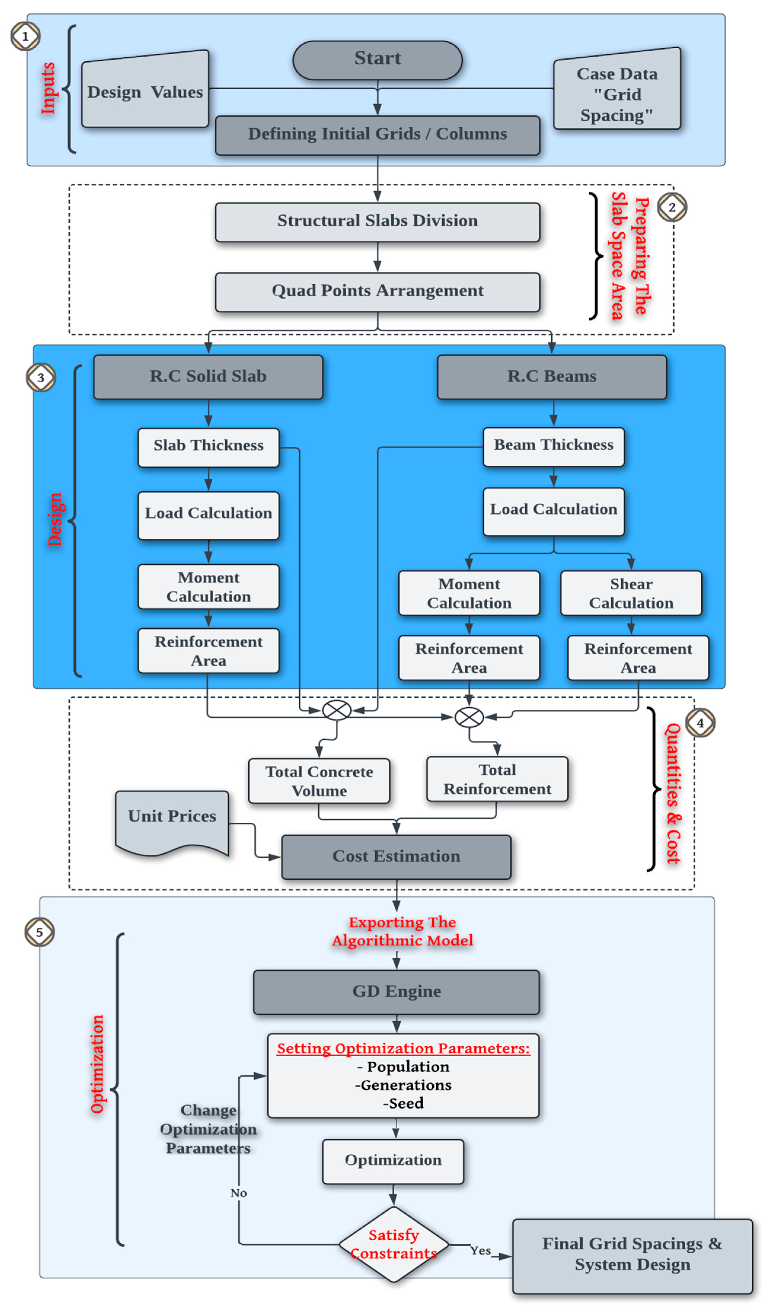
3. Model Development

This research presents a parametric model for optimizing the structural design of solid slab systems while maintaining architectural grid functionality. The model is developed within a BIM environment using Autodesk Revit 2024, with Dynamo^® 2.18.1 as the scripting platform and GD as the optimization engine. The algorithm is written in Design Script within the visual programming environment, enabling automated structural modeling and efficient design adjustments. The proposed framework follows a Cartesian grid system, where the architectural engineer defines space functions and dimensional constraints and the structural engineer inputs material properties, load limits, and design specifications based on industry codes (Figure 1). Column locations were predefined based on the architectural grid and integrated as fixed nodal supports within the structural model. These coordinates played a critical role in defining beam spans and support conditions throughout the optimization process, even though column sizing and detailing fell outside the scope of the current study. The model automates the generation of structural components, including grids, columns, floor spaces, slabs, and beams, while computing concrete volume, reinforcement quantities, and total system cost. In the optimization phase, a Genetic Algorithm (GA) integrated with GD refines the spatial layout to achieve optimal structural performance and material efficiency while preserving functional and architectural constraints. The subsequent sections detail the model development process. Although the current design rules are based on the Egyptian Code of Practice (ECP) [30], the proposed framework is highly adaptable and can be reconfigured to comply with other international codes, such as ACI 318 or Eurocode 2. This can be achieved by adjusting the input parameters and constraint values accordingly.

3.1. Conceptual Architectural System

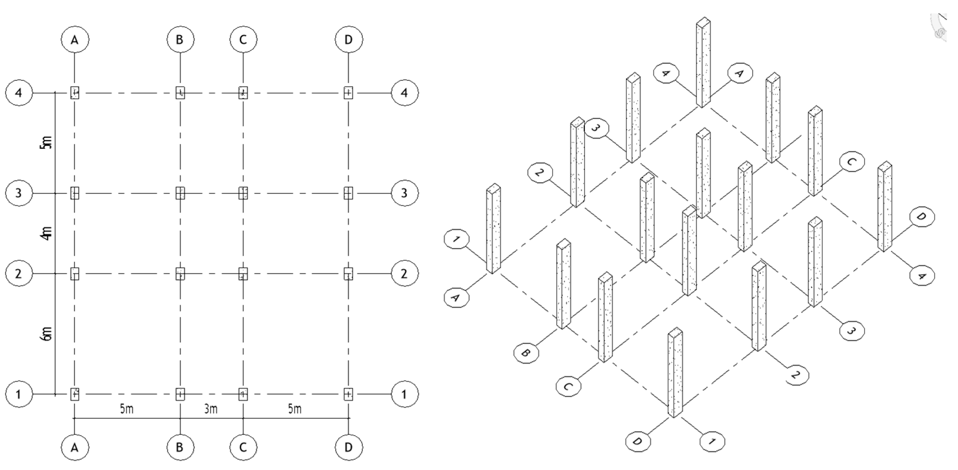
3.1.1. Defining Grids and Cartesian Points Arrangement

The model begins with defining a conceptual Cartesian grid system, where the architectural layout establishes the initial spatial configuration. Using Dynamo scripts within the Revit environment, horizontal and vertical grid lines are generated based on predefined spacing (Figure 2). These grids are then computationally interpreted as geometric vectors to determine column intersection points (IP). Each intersection point corresponds to a structural column location, forming the foundation for the subsequent placement of slabs and beams (Equation (1)). This automated grid generation ensures geometric consistency and alignment with architectural constraints, enabling a seamless transition to structural modeling (Figure 3).

$$IPs=\left[\begin{array}{ccc}{IP}_{11}& I_{12} \dots & I_{1z}\\ {IP}_{21}& I_{22} \dots & I_{2z}\\ ⋮& ⋮ \ddots & ⋮\\ {IP}_{r1}& I_{r2} \dots & I_{rz}\end{array}\right]$$

(1)

where z is the total IP number per grid line and r represents the total number of grids.

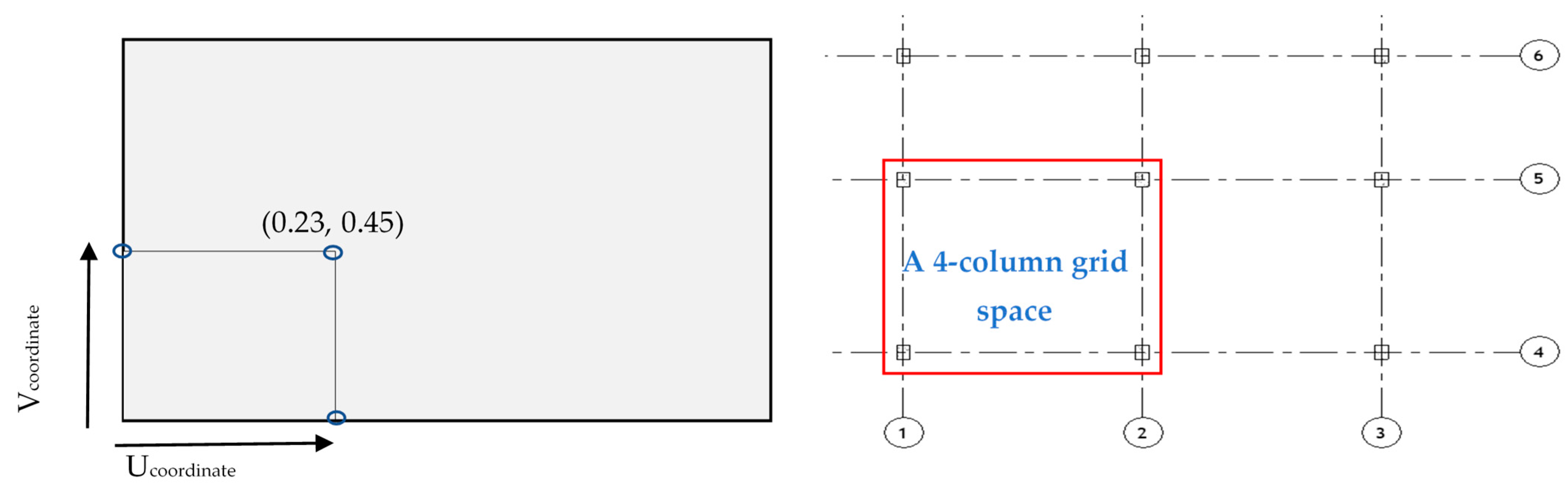
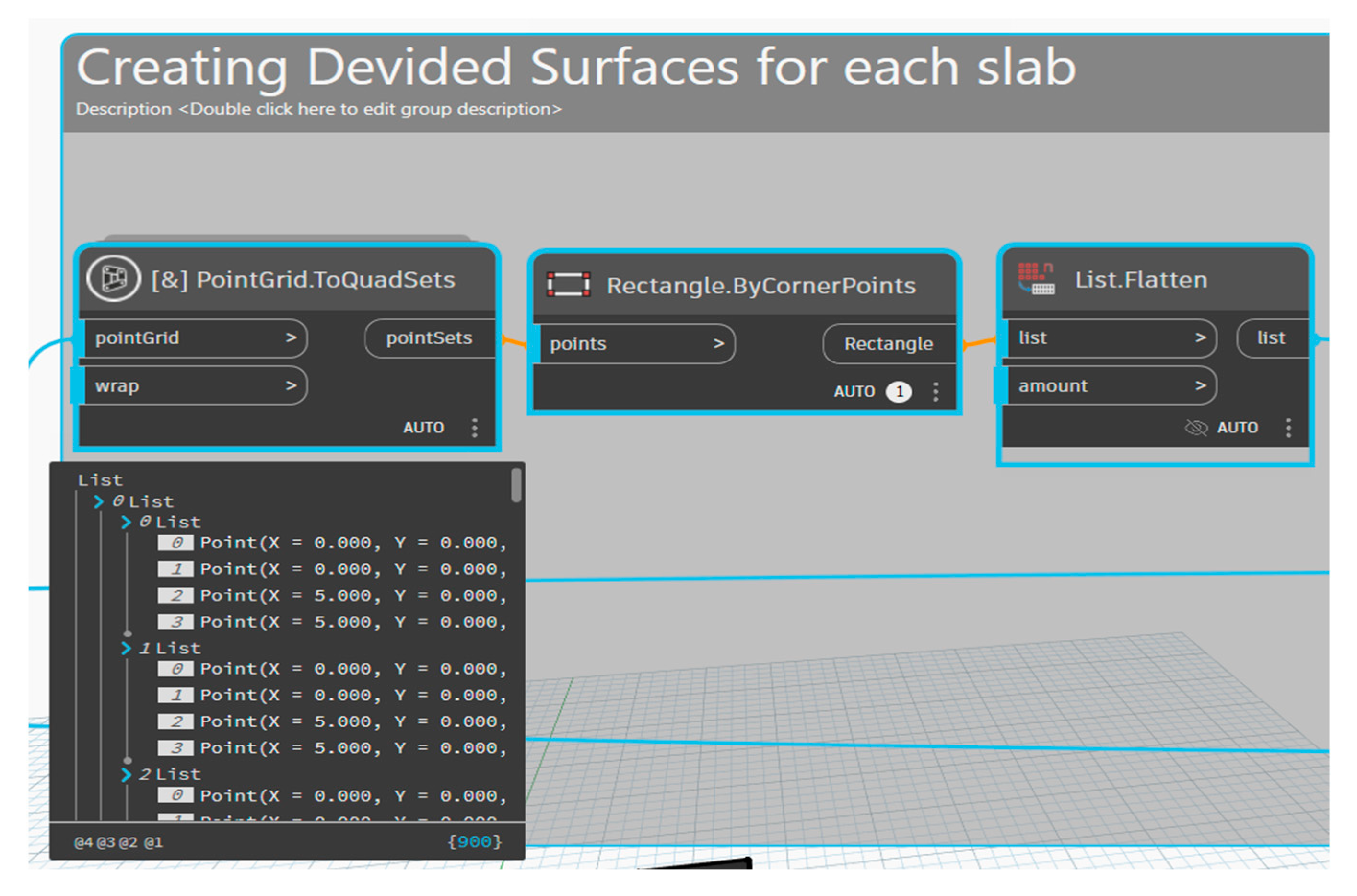
3.1.2. Structural Slab Division

The model divides the entire floor slab into smaller quadrilateral units, each bounded by four structural columns to facilitate structural analysis. This subdivision aligns with the predefined architectural grid and enables efficient assessment of loads, reinforcement, and slab thickness. The slab surface is parameterized to identify key geometric points, which are then grouped into quadrilateral sets representing individual slab panels [31]. This process ensures uniform structural discretization and supports subsequent automated calculations for design and optimization purposes, as illustrated in Figure 4 and Figure 5.

3.2. Structural Solid Slab Design

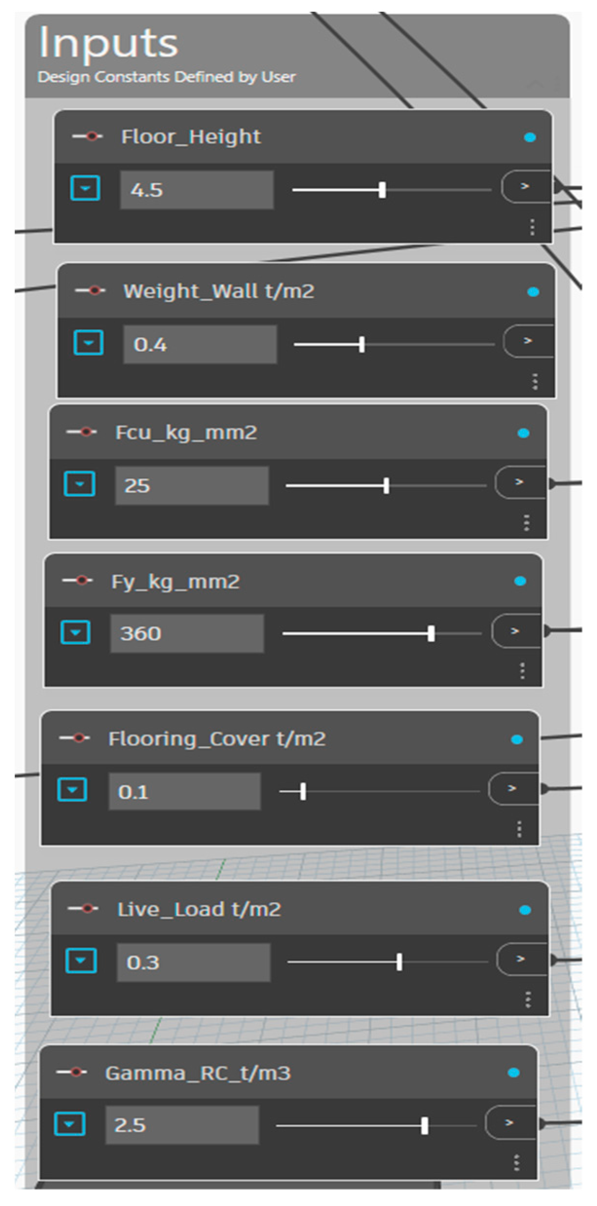
The structural design of the concrete solid slab system starts with the insertion of all design values, such as concrete properties, live load, flooring cover load, reinforcement properties, floor height, etc. (Figure 6). All input values can be customized according to the design needs; this customized change makes the model more generic so that it will apply to various architectural plans and structural design needs. The procedures followed in the design phase follow the ECP [30] and the computational analysis coding approach.

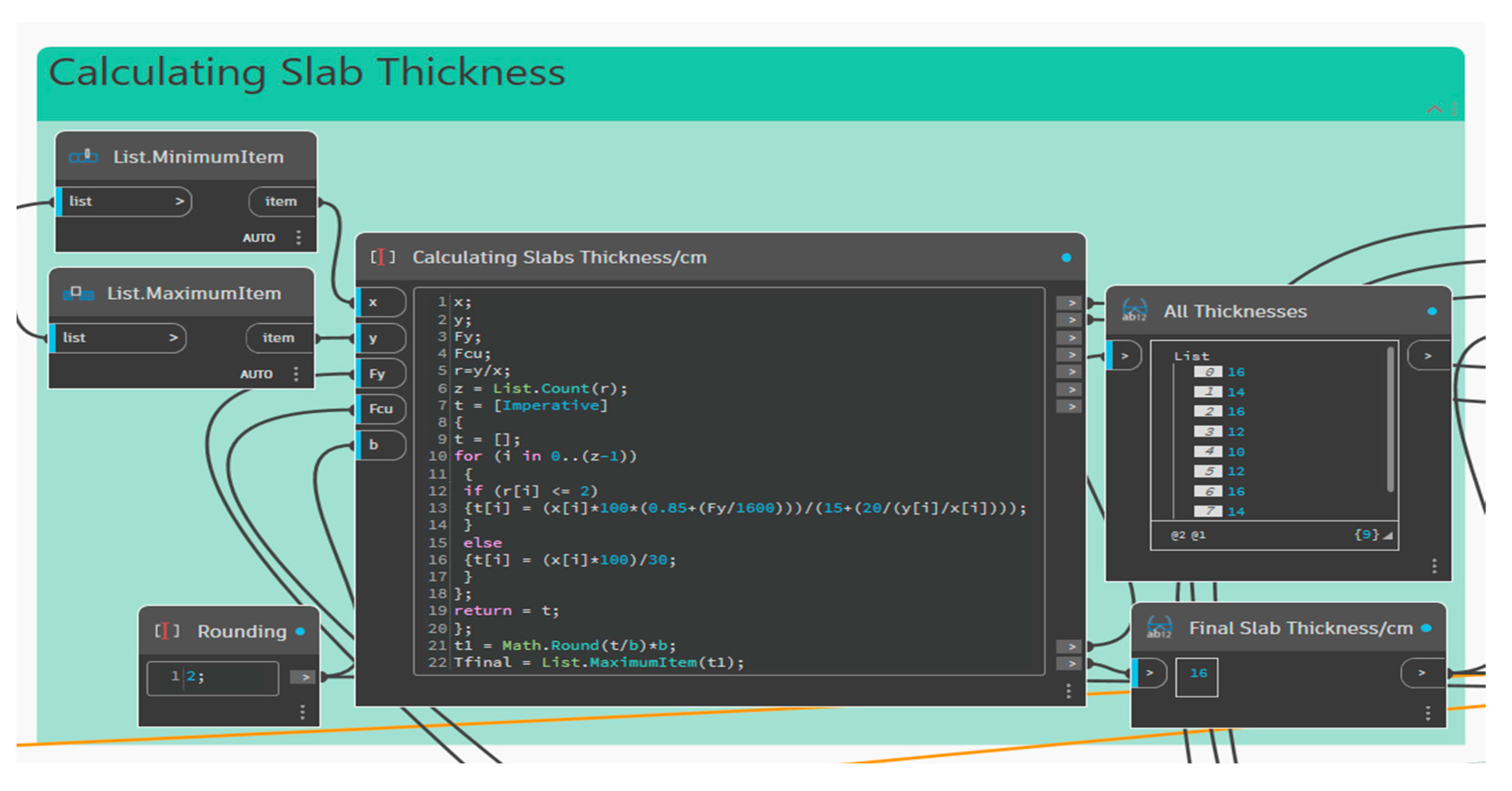
3.2.1. Structural Slab Thickness

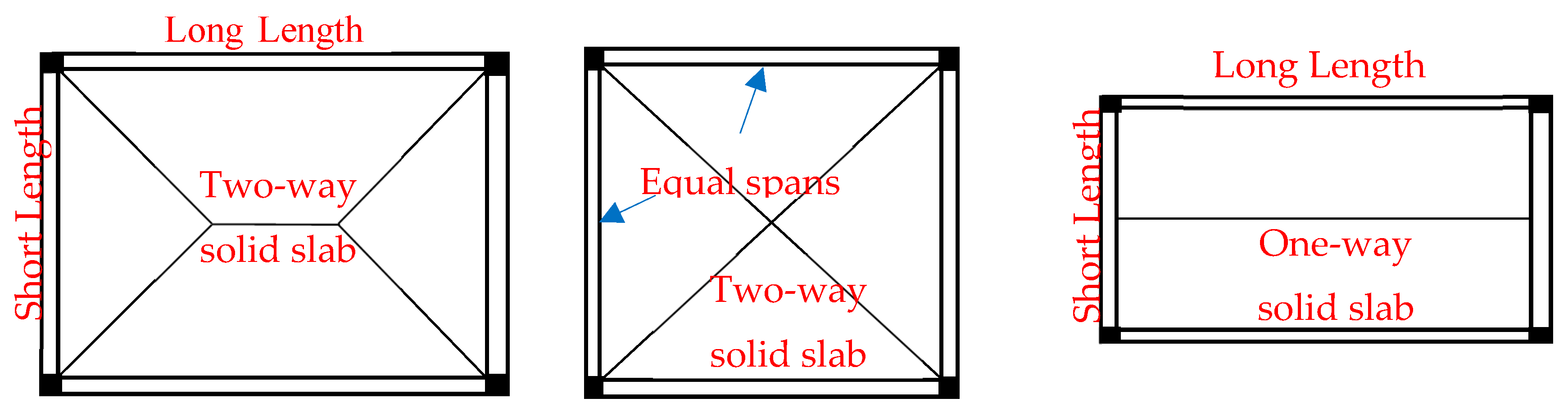
The width and length of each divided slab are retrieved to calculate the r-factor. According to the ECP [30], the r-factor is calculated by dividing the slab’s long dimension by its short one, and then this ratio is used to define the type of solid slab, which may be a one or two-way slab (Equation (2)). The type is determined according to the load distribution direction to the supporting beams within the context that each slab has four marginal beams. If the value of the r-factor is less than or equal to 2, then the slab is defined as a two-way slab. The slab is defined as one-way when the r-factor is more than 2.

$$r={\displaystyle \frac{L_l}{L_s}}$$

(2)

where L_l and L_s are the long and short slab dimensions.

According to the slab type, the structural thickness of each slab is calculated and rounded to the nearest 2 or 5 cm (Equations (3) and (4)). The floor slab system’s maximum thickness is unified (Figure 7).

$${\mathrm{t}}_{\mathrm{s}(\mathrm{one}-\mathrm{way})}=\left\{\begin{array}{c}\begin{array}{cc}{\displaystyle \raisebox{1ex}{$L$}\!\left/ \!\raisebox{-1ex}{$25$}\right.} & r>2, simple\end{array}\\ \begin{array}{cc}{\displaystyle \raisebox{1ex}{$L$}\!\left/ \!\raisebox{-1ex}{$30$}\right.}& r>2, continuous from one side \end{array}\\ \begin{array}{c}\begin{array}{cc}{\displaystyle \raisebox{1ex}{$ L$}\!\left/ \!\raisebox{-1ex}{$35$}\right.} & r>2, continuous from both sides\end{array}\\ \begin{array}{cc}{\displaystyle \raisebox{1ex}{$L$}\!\left/ \!\raisebox{-1ex}{$10$}\right.} & r>2, cantilever\end{array}\end{array}\end{array}\right.$$

(3)

where L is the short slab dimension.

$${\mathrm{t}}_{\mathrm{s}(\mathrm{two}-\mathrm{way})}={\displaystyle \frac{a(0.85+(\frac{F_y}{1600})}{15+\left(\frac{20}{\raisebox{1ex}{$b$}\!\left/ \!\raisebox{-1ex}{$a$}\right.}\right)+10\beta }}, r\le 2$$

(4)

where a is the short slab length, b is the long slab length, Fy indicates the yielding stress of the required steel, and β’ is the ratio of continuous edge length to the total perimeter of the slab.

3.2.2. Slab Load Calculation

According to the ECP, the RC solid slab’s ultimate load is calculated as illustrated in Equations (5) and (6) [30]. The load calculation depends on the summation of dead load (DL) and live load (LL) on the floor slab. The DL is the total weight of the concrete slab with its covering materials. The designer specifies the LL according to building type and usage.

W_u = 1.4 × DL + 1.6 × LL

(5)

DL = γ_concrete × t_s + F.C

(6)

where W_u is the total ultimate slab load, γ concrete represents the RC unit weight, ts is the solid slab thickness, and F.C is the flooring cover weight.

After the Wu has been calculated, the slabs are classified as “one-way” or “two-way” slabs according to another r′-factor value. As stated in Equation (7), the r′-factor is calculated considering the continuity of the slab in each direction (m₁ and m₂ values). In one-way slabs, all loads are transferred in a short direction. In two-way slabs, the loads are initially divided within the short direction and have the value of the ultimate slab load multiplied by a distribution factor “α” according to the ECP [30] (Equation (8)). The load transmitted through the long direction has the value of the ultimate slab load multiplied by a distribution factor “β” (Equation (9)). The r′-factor has a value of 1~2; if it is less than one, then use the reciprocal, and if it is more than two, then α will have a value of 1 while β will be equal to 0.

$$r\prime ={\displaystyle \frac{m_1\times L_l}{m_2\times L_s}}$$

(7)

α = (0.5 × (r′)) − 0.15

(8)

β = 0.35/(r′)²

(9)

where m₁ and m₂ are the distribution factors (equal to one if we are dealing with simple slab, 0.87 if continuous from only one edge, or 0.76 if continuous from both edges).

3.2.3. Calculations of Bending Moments in Solid Slabs

The model calculates the bending moment after determining loads on each slab direction. Figure 8 shows how the bending moment is calculated in solid slab strips according to the ECP for continuous and simple slabs.

3.2.4. Calculations of Areas of Steel Reinforcement in Solid Slabs

According to the ECP, the C₁-J curve calculates the required reinforcement area for sections subjected to the bending moment [30]. The developed model simplifies the curve into more usable values to complete the computational analysis by inserting the tabulated values next to the C₁-J curve as a list with a minimum limit of the C₁ value equal to 2.65 and a 4.85 maximum limit value (Equation (10)).

$$C_1-J \mathrm{values}=\left[\begin{array}{cc}{C}_{11}& J_{12}\\ \begin{array}{c}{C}_{21}\\ \begin{array}{c}⋮\\ C_{n1}\end{array}\end{array}& \begin{array}{c}{J}_{22}\\ \begin{array}{c}⋮\\ J_{n2}\end{array}\end{array}\end{array}\right]$$

(10)

where n is the number of C₁-J points (45 points from the chart).

The next step is calculating the required reinforcement area to withstand the applied moment. According to the ECP, Equation (11) is used to obtain the C₁ value, and then from the chart or table, the corresponding J value is obtained to be applied in Equation (12) and is used determine the total reinforcement area required [30]. The model rounds up all obtained C₁ values to the nearest “0.05” to obtain values close to those within the table.

$$d=C1\sqrt{{\displaystyle \frac{M_u}{f_{cu}\ast B}}}$$

(11)

$${\mathrm{A}}_{\mathrm{s}}={\displaystyle \frac{M_u}{f_y\ast J\ast d}}$$

(12)

where d is the adequate depth of the section (ts-slab cover), f_cu represents the ultimate stress of concrete, B is the moment strip width (slab = 1000 mm), and f_y represents the yielding stress of reinforcement steel.

3.3. Structural Beams Design

The developed model can be used to design the structural beam of the proposed slab system. It can calculate the loads transferred, the bending moment, and shear forces, and it can determine section dimensions with required reinforcement areas to withstand moment and shear. The following subsections describe the beams’ design process according to the ECP for concrete elements design.

3.3.1. Load Calculation

Concrete beams are the structural elements that carry the floor load and transfer it to the supporting columns. According to the ECP [30], the load on each beam is the sum of the beam’s weight, wall loads, and slab load (Equation (13)). As a one-way or two-way solid slab, the load area transferred from the slab to the beams depends on its type (Figure 9). The DL and LL from slab to beam are calculated by identifying the distributed area load and are summed according to the ECP ultimate limit method [30].

$$Bea{m}_{Loads}={\gamma }_{concrete}\ast t^{\prime }\ast b+Wal{l}_{Weight}\ast H_{wall}+g_s\ast \sum {\displaystyle \frac{Are{a}_{Load}}{L}}$$

(13)

where γ_concrete is the RC unit weight, t’ is the (beam depth − slab depth), b is the beam width, Wall_Weight is the user-defined weight of walls in t/m², H_wall is the (floor height − beam depth), g_s is the DL from the slab, Area_Load is the distributed area load from the slab to the beam, and L is the beam span.

3.3.2. Beam Bending Moment Calculation

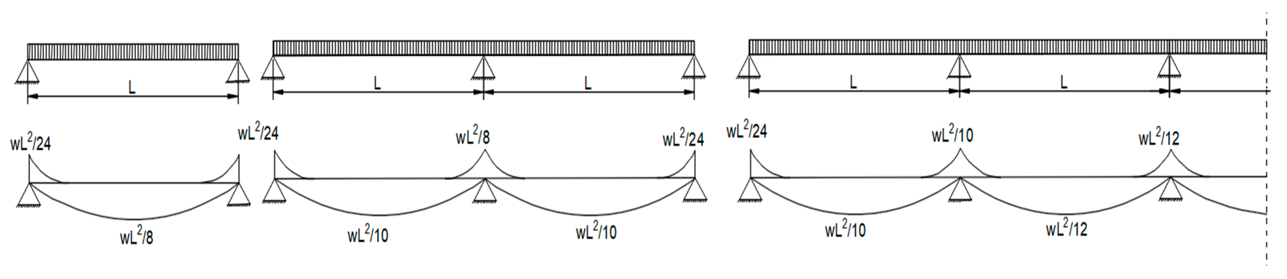
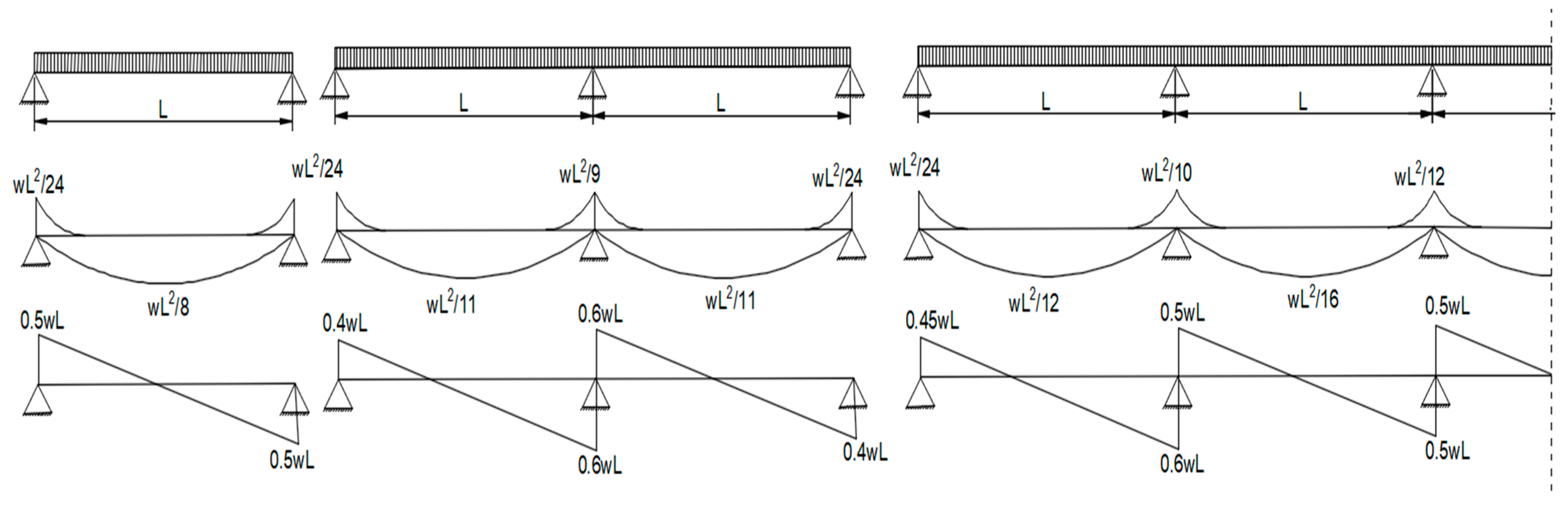
After defining the beam load, the next step is calculating the negative and positive moments. Figure 10 shows the ECP empirical values for moment and shear in concrete beams in the case of equal spans and loads. In the case of unequal spans or loads, negative moments are calculated according to the average values of consecutive lengths or load values.

3.3.3. Beam Reinforcement Area Calculation

Like the slab design procedures, beam design uses the C₁-J curve to calculate the required reinforcement area to withstand the applied bending moment (Equations (11) and (12)). The main differences are the “B” value (compression width from beam and slab) and “d” (beam depth) value used to calculate the C₁ value (Equation (11)).

$$q_{cu}=0.16\sqrt{{\displaystyle \frac{F_{cu}}{{\gamma }_c}}}$$

(14)

$$q_{u\_max}=0.7\sqrt{{\displaystyle \frac{F_{cu}}{{\gamma }_c}}}$$

(15)

$$q_u={\displaystyle \frac{Q_{max}}{bxd}}$$

(16)

$${\mathit{As}}_{\mathit{shear}}=\left\{\begin{array}{c}\begin{array}{cc}minimum 5@ 8/m\prime & q_u<q_{cu}\end{array}\\ \begin{array}{cc}{ q}_u-0.5 q_{cu}={\displaystyle \frac{{nA}_{st}\left(\raisebox{1ex}{$f_{yst}$}\!\left/ \!\raisebox{-1ex}{${\gamma }_s$}\right.\right)}{S.b}}& { q}_u>q_{cu} \&\& { q}_u<q_{u\_max} \end{array}\\ increase “d” { q}_u>q_{u\_max}\end{array}\right.$$

(17)

where $q_{cu}$ is the minimum shear stress on concrete sections, f_cu represents the ultimate stress of concrete, ${\gamma }_c$ is the concrete safety coefficient (equals 1.5), $q_{u\_max}$ is the maximum shear stress on concrete sections, d is the adequate depth of the beam’s section (t − cover), and $Q_{max}$ is the maximum shear force at the beam-critical section at a distance of d/2 from the column face. A_s shear represents the total shear reinforcement area, f_yst represents the yielding stress of reinforcement steel for the stirrups, and m is the number of spans in each beam in a specified direction.

Shear stresses are calculated according to the ECP [30], where the actual shear stress is compared to the minimum and maximum shear stresses on concrete sections to calculate shear reinforcement areas (Equations (14)–(17)). All calculated reinforcement areas are in square millimeters.

3.4. Preparing Quantities and Calculating Cost

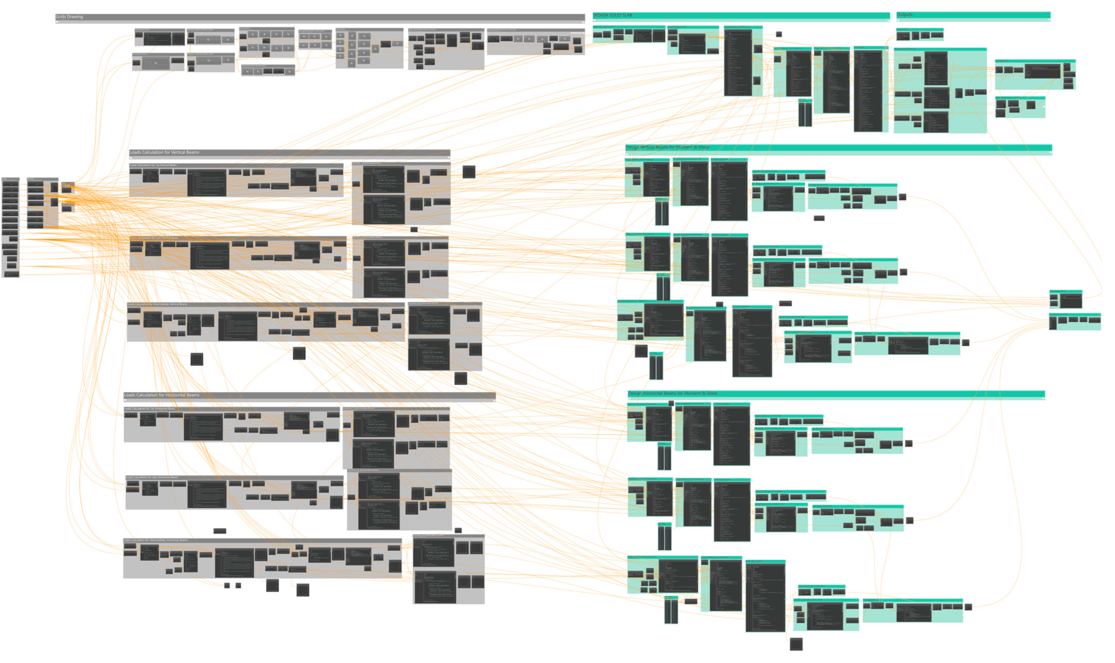
Figure 11 shows the parametric algorithm that has been developed to define, analyze, and design any solid slab system within the BIM environment. The Dynamo flows from left to right, starting with defining the design parameters, calculating slab thickness, loads, and moment, and then determining the reinforcement area needed to cover the slab area. To calculate the cost of the solid slab floor system (concrete and reinforcement), the model first calculates the concrete volume by multiplying the total slab area by its designed thickness.

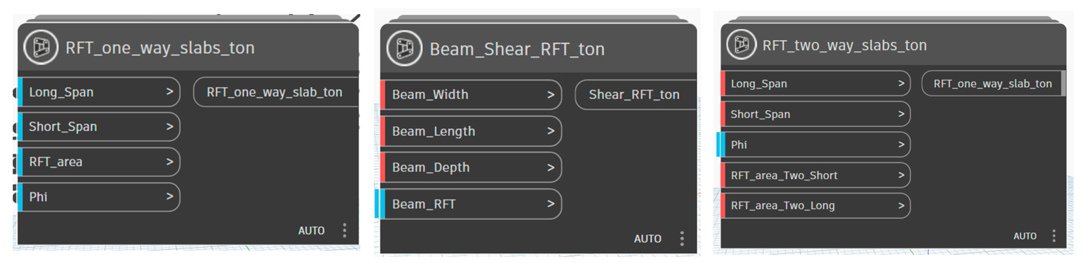
To calculate the reinforcement cost, all the reinforcement areas calculated for slabs and beams must be converted to weights in tonnage and multiplied by their market price. The authors have developed some ready-made custom nodes to complete this job and convert steel areas into weights (Figure 12). This is mainly achieved by multiplying the number, length, and unit weight of the reinforcement required for each section. The overall price is given by multiplying the quantity of reinforcement and the unit price (defined by the user). The designed reinforcement areas include steel required for slabs and beams used for bending and shear.

3.5. Generative Design Optimization

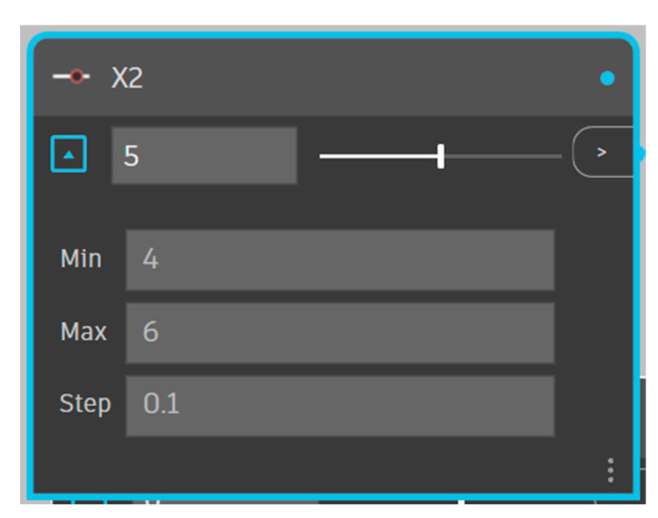
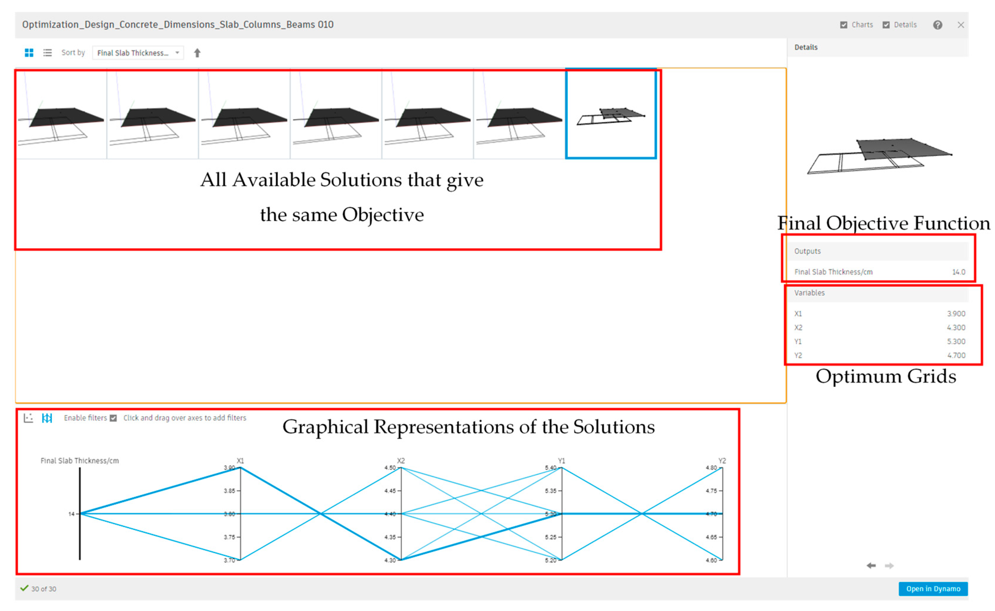
Generative design (GD) is an advanced optimization approach within the BIM environment that minimizes total system cost by refining grid spacing. The optimization algorithm adjusts X and Y dimensions within predefined upper and lower limits, which the architect sets based on functional requirements. The model evaluates concrete volume (m³) and reinforcement weight (tons) to determine the most cost-efficient configuration. Grid spacing variations are optimization variables, allowing the system to identify the optimal design iteratively. For instance, if the initial vertical grid spacing is 5 m, with a ±1 m tolerance, the algorithm explores values between 4m and 6m to achieve the lowest material cost (Figure 13).

Defining the Optimization Problem

In this study, the objective function is to minimize the total cost of material (Equation (18)), where the optimization engine changes the grid distances through predefined functional limits set by the architect.

TC = UR_concrete × V_concrete + UR_RFT × W_RFT

(18)

where TC is the total material cost of the slab system (concrete and steel), UR_concrete is the unit rate of concrete, V_concrete is the total concrete volume in the system (slabs + beams), URRFT is the unit rate of reinforcement, and WRFT is the total weight of reinforcement for slab and beams (moment and shear reinforcement).

The optimization variables are the grid distances (Equations (19) and (20)). The process gives all available optimum grid distances that provide the minimum objective (total material cost). The GD engine provided by Revit is very flexible and practical, and can be applied to any targeted optimization objective.

$$X_{\mathit{spacing}}=\left[\begin{array}{ccc}{x}_1& \begin{array}{cc}{x}_2& \dots \end{array}& x_s\end{array}\right]$$

(19)

$$Y_{\mathit{spacing}}=\left[\begin{array}{ccc}{y}_1& \begin{array}{cc}{y}_2& \dots \end{array}& y_t\end{array}\right]$$

(20)

where x and y represent the grid distances (variables) and s and t are the total number of spacings in both directions.

In this case, the constraint is to keep the overall width and length (L1 and L2) constant. To allow the model to satisfy the defined constraint, a penalty is applied to the total cost value by multiplying it by an enormous number so that the model tries to satisfy the constraint and obtain the length and width constant.

4. Application and Case Studies

4.1. Case Study 1

A floor plan example validated the proposed visual parametric model (Figure 14). The grid dimensions were set to 3.2 m and 5 m in the X-direction (total width: 8.2 m) and 6 m and 4 m in the Y-direction (total length: 10 m). To assess the model’s accuracy, the slab system was manually designed using the exact grid dimensions, and the results were compared with the model’s calculations for both slabs and beams. As shown in

Table 2. Model validation: “manual design vs. automatic design” case study 1.

No.	Manual Design	Automatic Design
Slab Design Values
Thickness	16 cm	16 cm
Loads	1.18 t/m2	1.18 t/m2
Reinforcement	Minimum (5 ɸ 10/m′)	392.69 mm2 (5 ɸ 10/m′)
Beam Design Values
Beam depth	45 cm	45 cm
Loads	3.44 t/m′, 4.56 t/m′	3.45 t/m′, 4.57 t/m′
Reinforcement	2 ɸ 12	113.1 mm2~2 ɸ 12
Shear Stirrups	Minimum (5 ɸ 10/m′)	Minimum (5 ɸ 10/m′)

Note: Beam validation was checked with the intermediate horizontal beam.

, the model’s output perfectly aligned with manual design values, confirming its validity and reliability for the structural design calculations. This configuration was intentionally simplified to serve as a controlled validation scenario, enabling precise benchmarking of the model’s performance.

The next step involved testing the practicality of the optimization process.

Table 3. Optimization case scenarios: “test the model”.

No.	Objective Function	Initial Value	Optimum Value	Variables
Case I	Minimize the slab thickness	16 cm	14 cm	X: (3.9, 4.3) Y: (5.4, 4.6)
Case II	Minimize the system design cost	EGP 76,513	EGP 63,488	X: (4, 4.2) Y: (5.4, 4.6)

Note: Unit rates are considered as follows: “EGP 10,000/ton for Reinforcement” and “EGP 2000/m³ for Concrete.”

presents two validation scenarios for the GD optimization engine. In each scenario, grid dimensions were allowed to vary by ±1 m, a range that can be adjusted based on the designer’s preferences.

• Scenario 1: Slab Thickness Optimization—the aim was to determine the optimal grid dimensions that minimize only the concrete slab thickness.
• Scenario 2: System Cost Optimization—the aim was to minimize the total system costs by optimizing concrete and reinforcement quantities.

The optimization process was applied on a computer desktop running the operating system Microsoft Windows 10, an Intel Core i7 processor at 2.7 GHz, and 32 GB of RAM. The Dynamo visual algorithm was exported to the GD engine, where key parameters were set:

• Thirty generations.
• One hundred and fifty individuals per generation.

The GD engine successfully identified the optimal grid configuration (Figure 15), yielding a 14 cm solid slab thickness as the most cost-effective solution for the first scenario (Table 2). The second optimization scenario focused on determining the optimal system dimensions to minimize the total design cost of the solid slab system. The model aimed to identify the optimal grid spacing, resulting in the lowest material consumption while maintaining structural integrity. The initial slab dimensions provided a system design with a slab thickness of 16 cm and EGP 76,513 for the total material cost (concrete and reinforcement). This design was successfully optimized to have a 14 cm slab thickness, a 17% reduction in material cost, and a total final cost of EGP 63,488. These results confirm that the proposed Dynamo-GD model is a practical and scalable solution for optimizing solid slab designs, with potential applications across various floor plans.

The optimization process was executed efficiently across all scenarios, with reasonable computational time and system performance. As the complexity of the optimization increased, the processing time rose from 120 s in the first scenario to 600 s in the second due to additional computational dependencies and variables.

4.2. Case Study 2

The second case study involves a one-story chalet, where the proposed structural system consists of a solid slab supported by 12 concrete columns (Figure 16). The architectural grid spacing and all of the design parameters were incorporated into the optimization algorithm to minimize total system costs, including concrete and reinforcement usage. The initial floor design featured a grid spacing of 3.5 m × 3.5 m in the X-direction and 4.5 m, 3.4 m, and 3.8 m in the Y-direction. Based on the designer’s preference, all dimensions were assigned an adjustable range of ±1 m to allow flexibility in the optimization process. The initial cost of the structural system was EGP 357,000. To refine the design, the optimization process was conducted through multiple trials, varying population sizes, and each trial iteration. As shown in

Table 4. Optimized targeted objective “% savings” case study 2.

	Variables	Material Cost (EGP)	Slab Thickness/cm	Concrete/m3	Reinforcement/ton
Original	X: (3.5, 3.5) Y: (4.5, 3.4, 3.8)	357,000	12	15.5	4.5
Optimized Values	X: (3.6, 3.4) Y: (4.1, 3.6, 4)	347,200	12	15	4.4
% Savings	--	2.7%	--	3.8%	2%

Note: Unit rates are considered as follows: “EGP 38,000/ton for reinforcement” and “EGP 12,000/m³ for concrete.”

, the final optimized design resulted in a total cost reduction of EGP 347,200, achieving a 2.7% cost savings. Material consumption was also optimized, leading to 3.8% savings in concrete and 2% in reinforcement. Given the structure’s scale, the savings percentages may vary for larger or more complex projects. However, the results confirm the model’s efficiency in reducing material costs and optimizing grid dimensions, demonstrating its applicability across different structural configurations.

4.3. Case Study 3

The third case study examined a multi-story building where the structural system consisted of a solid slab supported by concrete columns on each of its eight floors (Figure 17). The optimization aimed to minimize material costs by adjusting the grid spacing while maintaining structural integrity. The initial design had grid spacing of (5, 6, 5.5, 4) m in the X direction and (5, 5.2, 4.2) m in the Y direction, resulting in an 18 cm slab thickness. The material cost of this initial design was EGP 1,409,710.4 for each floor slab.

Twenty optimization trials were conducted to refine the design and determine the optimum grid dimensions, varying population sizes, and the total number of iterations. The optimum grid spacings were (5.1, 5.4, 5.2, 4.8) in the X direction and (4.6, 5.4, 4.4) in the Y direction. This reduced the slab thickness to 16 cm, decreasing the slab material cost to EGP 1,274,546.22 for each floor. The optimization resulted in a 9.58% reduction in total cost and savings of 9.69% in concrete volume and 9.43% in reinforcement quantity (

Table 5. Optimized targeted objective “% savings” case study 3.

	Variables	Material Cost (EGP)	Slab Thickness/cm	Concrete/m3	Reinforcement/ton
Original	X: (5, 6, 5.5, 4) Y: (5, 5.2, 4.2)	1,409,710.4	18	71.486	14.523
Optimized Values	X: (5.1, 5.4, 5.2, 4.8) Y: (4.6, 5.4, 4.4)	1,274,546.22	16	64.557	13.154
% Savings	--	9.58%	--	9.69%	9.426%

Note: Unit rates are considered as follows: “EGP 38,000/ton for reinforcement” and “EGP 12,000/m³ for concrete.”

). The processing time for this case study was 930 s due to the increased number of variables being considered.

5. Results and Discussion

The performance of the proposed Dynamo-based optimization framework was evaluated through three representative case studies, each exhibiting different spatial scales, design constraints, and load configurations. The results in

Table 6. Comparison of optimization results in case studies.

Optimization Factor	Case Study 1	Case Study 2	Case Study 3
Initial Cost (EGP)	76,513	357,000	1,409,710
Optimized Cost (EGP)	63,488	347,200	1,274,546
Total Cost Savings (%)	17%	2.7%	9.58%
Concrete Savings (%)	13.38%	3.8%	9.69%
Reinforcement Savings (%)	20.87%	2%	9.426%
Computational Time (sec)	120–600	620	930

reflect the model’s capacity to improve material efficiency and reduce structural costs through adaptive grid spacing optimization. The outcomes are interpreted in terms of material savings, computational behavior, and potential for broader structural application, within the scope and assumptions defined earlier in Section 3.

Using geometrically regular configurations in the presented case studies was a deliberate methodological choice to isolate the model’s optimization capabilities under controlled vertical load scenarios. These configurations reflect common early-stage design conditions, providing a reliable basis for validating material savings and cost-efficiency before extending the model to irregular or laterally governed systems.

5.1. Optimization Performance Across Case Studies

Table 6 presents the results of the initial and optimized scenarios across the three case studies. In each case, the optimization process yielded quantifiable reductions in total material cost, concrete volume, and reinforcement quantities. In case study 1, which featured a uniform grid layout and minimal architectural constraints, the optimization algorithm achieved the highest reduction in material usage, suggesting that early-stage models with greater geometric flexibility yield the most substantial improvements. Conversely, case study 2, a low-rise chalet with fixed spatial partitions, showed limited optimization potential. The lower savings percentages in that case highlight how architectural rigidity and functional zoning can constrain grid adaptability, thereby limiting structural optimization leverage. Case study 3, representing a multi-story commercial building, demonstrated intermediate performance gains and a longer processing time, reflecting the added complexity and design variables associated with vertical stacking and increased load scenarios. These results reinforce the model’s sensitivity to geometric and architectural variability and its practical capacity to deliver savings in typical mid- to large-scale structural layouts.

5.2. Interpretation of Computational Behavior

The algorithm maintained computational stability across design scenarios, with total optimization durations ranging from approximately 120 to 930 s. In case study 1, optimizing slab thickness and column locations converged rapidly due to the relatively constrained solution space. Case studies 2 and 3 required longer runtimes, and this was attributed to additional design constraints and a larger set of optimization variables.

Despite these differences, the model’s processing times remain acceptable within typical schematic design timelines, positioning it as a viable decision-support tool during early planning. The performance stability suggests that the GD algorithm, implemented within Dynamo, can handle moderate- to high-complexity optimization tasks without requiring significant hardware resources or computation tuning.

5.3. Structural Logic and Practical Insights

The model’s optimization strategy focused on grid spacing adaptation to reduce material usage, primarily by controlling slab spans and reinforcement patterns. While this approach does not incorporate advanced interaction effects, such as slab–column punching shear, torsional stiffness, or soil–structure interaction, it still provides a reliable proxy for early-stage material estimation and cost benchmarking. The simplifications adopted (e.g., exclusion of seismic, dynamic, or lateral forces) were deemed appropriate for the model’s scope as a conceptual optimization tool rather than a detailed structural analysis engine.

Although the current model primarily addresses rectilinear configurations, its parametric foundation allows future extensions to accommodate irregular load paths and unconventional column–beam interactions. Moreover, the selected case studies, while limited to orthogonal, regular grids, served to validate the model’s baseline functionality and optimization potential. The current implementation’s absence of irregular geometries, voids, or eccentric load paths represents a recognized limitation. Future extensions should incorporate structural irregularities, cantilevered slabs, or non-rectilinear layouts to assess the robustness of the optimization process under more diverse architectural conditions.

5.4. Broader Applicability and Future Extensions

Despite its constraints, the proposed optimization model demonstrates notable scalability, automation, and adaptability strengths. It maintained computational efficiency across different building scales and complexity levels, indicating its potential applicability to various structural design scenarios. Using a parametric workflow significantly reduced the need for manual intervention, enabling rapid and iterative exploration of alternative configurations. Although the present study focuses primarily on slab systems, minimal parameter modifications can readily adapt the underlying framework to other structural components, such as footings, beams, or precast elements. To further enhance the model’s generalizability and structural fidelity, when working on future developments, researchers should consider integrating nonlinear finite element solvers for detailed stress verification, adopting multi-objective fitness functions that balance cost, deflection, and environmental impact, and incorporating reinforcement-detailing algorithms to ensure automated compliance with relevant structural codes.

Also, future development of the framework will include handling structural irregularities such as eccentric supports and beam-supported columns, enabling the model to address a broader range of building typologies and design practices. Furthermore, extensions of the proposed model could involve the integration of alternative design codes. The flexible parametric structure supports this transition, making it applicable to a broader range of regulatory contexts and enhancing its global usability.

6. Conclusions

This study presents a parametric algorithmic model for designing and optimizing solid slab structural systems, integrating it with rectilinear architectural layouts to achieve efficient and functionally viable solutions. Developed within the Dynamo for Revit environment, the model leverages generative design (GD) as its optimization engine to explore multiple design alternatives while ensuring compliance with structural and architectural constraints. The proposed approach enhances design efficiency in reinforced concrete (RC) buildings by automating key processes and optimizing material usage and grid configurations. A case study evaluation validates the model’s feasibility, demonstrating its effectiveness in reducing material costs and refining grid layouts for improved structural performance. However, the methodology focuses exclusively on vertical load conditions and regular slab configurations; it does not incorporate seismic loading or account for complex, irregular geometries. These limitations define the scope of applicability for the current framework and represent areas for future enhancement. Future research could extend this model into a Revit add-in with a user-friendly interface, allowing designers to modify design parameters and constraints easily. Expanding its capabilities to more complex structural systems, such as footings, shear walls, and multi-story frameworks, would further enhance its applicability. Integrating advanced optimization techniques and AI-driven predictive analytics could also drive future advancements in automated structural design within the construction industry.