Interpretable Machine Learning Framework for Non-Destructive Concrete Strength Prediction with Physics-Consistent Feature Analysis

Abstract

Non-destructive concrete strength prediction faces limitations in validation scope, methodological comparison, and interpretability that constrain deployment in safety-critical construction applications. This study presents a machine learning framework integrating polynomial feature engineering, AdaBoost ensemble regression, and Bayesian optimization to achieve both predictive accuracy and physics-consistent interpretability. Eight state-of-the-art methods were evaluated across 4420 concrete samples, including statistical significance testing, scenario-based assessment, and robustness analysis under measurement uncertainty. The proposed PolyBayes-ABR methodology achieves R² = 0.9957 (RMSE = 0.643 MPa), showing statistical equivalence to leading ensemble methods, including XGBoost (p = 0.734) and Random Forest (p = 0.888), while outperforming traditional approaches (p < 0.001). Scenario-based validation across four engineering applications confirms robust performance (R² > 0.93 in all cases). SHAP analysis reveals that polynomial features capture physics-consistent interactions, with the Curing_age × Er interaction achieving dominant importance (SHAP value: 4.2337), aligning with established hydration–microstructure relationships. When accuracy differences fall within measurement uncertainty ranges, the framework provides practical advantages through enhanced uncertainty quantification (±1.260 MPa vs. ±1.338 MPa baseline) and actionable engineering insights for quality control and mix design optimization. This approach addresses the interpretability challenge in concrete engineering applications where both predictive performance and scientific understanding are essential for safe deployment.

1. Introduction

Concrete compressive strength (CCS) is fundamental to structural engineering, directly impacting infrastructure safety and durability [1,2]. While comprehensive concrete characterization encompasses multiple properties, including tensile strength, durability parameters, and permeability, compressive strength serves as the primary structural design parameter in concrete engineering practice [3,4]. This study focuses on compressive strength prediction as the most critical mechanical property for structural applications.

Non-destructive evaluation (NDE) of CCS presents challenges due to concrete’s inherent heterogeneity and complex nonlinear behavior. Traditional CCS evaluation relies on destructive testing methods that, while reliable, are time-consuming and damage structural components [5]. These methods cannot capture spatial variability across large concrete elements, which NDE techniques can address [6].

Individual non-destructive testing (NDT) methods have limited accuracy due to concrete heterogeneity, nonlinear behavior, and sensitivity to mix designs and moisture content [7,8]. Combined approaches using multiple NDT techniques enhance prediction accuracy, often integrating surface hardness, ultrasonic pulse velocity (UPV), and penetration resistance with statistical methods like response surface methodology [7]. However, such approaches typically employ simplified regression models that inadequately capture complex nonlinear interactions among material, environmental, and testing parameters.

Traditional linear and multivariate regression methods cannot model the complex nonlinear behavior in concrete materials, particularly under diverse curing conditions and mix designs [9]. Research by Sah and Hong [9] comparing four machine learning (ML) models for concrete strength prediction found artificial neural networks most effective, followed by support vector machines, regression trees, and multivariate linear regression, confirming the limitations of traditional linear methods. Polynomial regression techniques address these limitations. Imran et al. [10] demonstrated significant improvements in predictive performance through multivariate polynomial regression by capturing nonlinear interactions among critical variables.

ML has significantly advanced CCS prediction by effectively modeling nonlinear relationships within material behavior. Advanced algorithms like Random Forest, gradient boosting, and neural networks consistently outperform traditional models by capturing complex interactions [11,12]. These approaches have shifted structural health monitoring from reactive to proactive paradigms [1], with ensemble models particularly excelling at managing data noise [13,14,15]. Among ensemble techniques, AdaBoost has gained attention for iteratively refining weak learners, with Ahmad et al. [16] demonstrating its effectiveness for predicting concrete strength under various conditions.

Research by Kioumarsi et al. [11] and Nguyen and Ly [17] tested advanced models on high-performance concrete, achieving lower errors and higher accuracy than conventional approaches. Multiple investigations confirm that ensemble techniques deliver consistently higher prediction accuracy and generalizability [18,19,20,21,22,23].

Polynomial feature expansion effectively captures nonlinear correlations in complex datasets. Imran et al. [10] demonstrated the advantages of polynomial features over linear and support vector regression, while Leng et al. [24] integrated polynomial features into an AdaBoost framework to address concrete microstructure modeling challenges. Recent studies show advancements in ML for CCS prediction, with Hoang et al. [1] developing interpretable models using UPV and mix design parameters, and Elhishi et al. [13] demonstrating XGBoost performance while identifying cement content and age as dominant features.

Recent advances in computational modeling for concrete engineering have progressed through physics-informed neural networks (PINNs), hybrid ML approaches, and uncertainty-aware frameworks. Varghese et al. [25] demonstrate how embedding fundamental cement hydration principles directly into neural network architectures enhances strength prediction accuracy, achieving 26.3% RMSE improvement while maintaining robustness with limited training data. Lee and Popovics [26] leveraged wave propagation physics to characterize material inhomogeneity, enabling non-destructive Young’s modulus evaluation with sub-4% error for quality control in layered concrete systems.

Hybrid methodologies bridge computational efficiency and predictive reliability. Asteris et al. [27] developed an ensemble meta-model integrating five ML techniques, attaining a testing R² of 0.8894 while addressing physical consistency issues at extreme mix proportions. Chen et al. [28] combined support vector machines and artificial neural networks through genetically optimized weighting, reducing carbonation depth prediction errors by 50% compared to standalone models. However, PINNs often require extensive domain expertise for physics equation formulation, while hybrid mechanistic models may suffer from computational complexity in practical deployments.

The interpretability–performance trade-off in ML has been challenged by Kruschel et al. [29], who demonstrated that the assumed strict trade-off between model performance and interpretability represents a misconception, suggesting that high-performing models can maintain interpretability without significant performance degradation. However, achieving this balance requires careful feature engineering and validation approaches that align with domain knowledge. This finding is particularly relevant to concrete engineering, where Ekanayake et al. [30] treated SHAP (Shapley Additive Explanations) as a “novel approach” for explaining concrete strength prediction models, indicating underutilization of interpretability techniques in the field.

Uncertainty quantification has emerged as important for risk-sensitive structural decisions. Tamuly and Nava [31] established statistically rigorous prediction intervals via conformal frameworks, achieving 89.8% empirical coverage for high-performance concrete applications. Ly et al. [32] implemented Monte Carlo techniques within optimized neural networks, generating confidence bounds that enhanced reliability for self-compacting concrete applications.

Hyperparameter tuning is important for optimal performance in complex models. Bayesian optimization has emerged as a resource-efficient alternative to exhaustive searches, guiding parameter selection to mitigate overfitting [33,34]. Joy [34] applied this approach to enhance models for predicting concrete strength, improving prediction accuracy, while Abazarsa and Yu [6] reported that Bayesian optimization reduced tuning time while enhancing prediction outcomes.

Several gaps persist in current approaches to non-destructive concrete strength evaluation. Most existing models fail to capture the complex nonlinear interactions among material parameters, environmental conditions, and NDE measurements. Few studies effectively integrate multiple NDE techniques with categorical mix design information in a unified predictive framework. The balance between model complexity, interpretability, and computational efficiency remains inadequately addressed for practical field applications.

Most studies suffer from limited validation scope, typically comparing against 2–3 baseline methods without statistical testing, and insufficient comparison with state-of-the-art gradient boosting methods (XGBoost, LightGBM) that have become industry standards. An analysis by Altuncı [35] of over 2300 articles on ML-based strength prediction confirmed these gaps while highlighting persistent challenges in data scarcity and model explainability.

This research addresses these limitations through an interpretability framework that achieves competitive performance while providing physics-consistent insights for practical engineering applications. The study provides a comparison against eight state-of-the-art methods, including XGBoost, LightGBM, Random Forest, neural networks, and traditional approaches, supported by statistical significance testing and effect size analysis.

The methodology incorporates concrete materials science principles through feature engineering, considering cement hydration kinetics governing time-dependent strength development, microstructural evolution reflected in electrical resistivity (ER) measurements, elastic property development captured through UPV, and pore structure formation influencing both mechanical and transport properties. Post hoc analysis validates the physics-consistency of the discovered relationships, connecting statistical performance with engineering understanding.

Model performance is evaluated across diverse engineering scenarios, including high-strength concrete, early-age applications, extended curing, and low resistivity conditions to assess generalization capability. The analysis evaluates model behavior under measurement noise and compares robustness across different algorithms, providing practical insights for field deployment.

2. Methodology

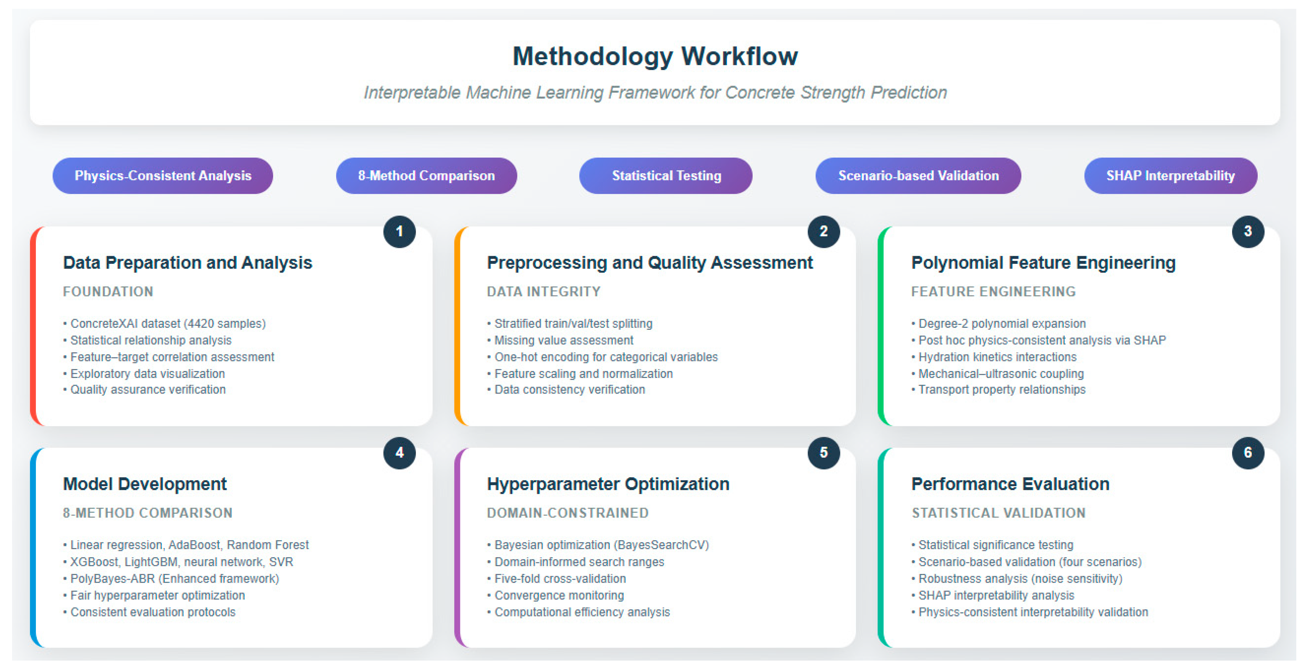
This section presents a framework for developing and validating interpretable ML for CCS prediction. The approach follows a structured workflow: (1) data preparation and analysis, (2) preprocessing and quality assessment, (3) polynomial feature engineering, (4) model development, (5) hyperparameter optimization, and (6) performance evaluation with physics-consistent interpretability analysis. Figure 1 illustrates the complete methodology workflow, emphasizing feature engineering with advanced ML techniques to achieve both accuracy and engineering interpretability.

2.1. Data Preparation

2.1.1. Dataset Characteristics

The analysis employed the ConcreteXAI dataset [36] consisting of 4420 concrete samples publicly available at https://github.com/JaGuzmanT/ConcreteXAI (accessed on 22 February 2025). This dataset provides diversity for model training and validation within the scope of the included concrete types, encompassing specimens with varying compositions, curing conditions, and strength properties across engineering applications.

Each data instance includes both categorical and numerical predictors collected through NDE and testing protocols. The integration of categorical mix design information (cement type, brand, additives, aggregate types) with quantitative measurements (design strength, curing age, ER, UPV) ensures representation of factors influencing concrete strength development.

Table 1. Comprehensive descriptive summary of dataset variables.

Feature	Type	Description	n	Missing Data
Type of cement	Categorical	CPC 30R (29.4%), CPO 30R RS BRA (29.0%), CPC 30R RS (21.7%), CPC 40R (19.9%)	4420	0%
Brand	Categorical	CEMEX (80.1%), Apasco (19.9%)	4420	0%
Additives	Categorical	No_additions (45.7%), Opuntia_ficus_indica (25.3%), Blast_furnace_slag_10% (14.5%), Starch_fluidizer (7.2%), fluidizer (7.2%)	4420	0%
Type of aggregates	Categorical	Crushed (34.8%), Rounded (29.0%), Recycled (29.0%), Volcanic (7.2%)	4420	0%
Design_F′c (MPa)	Numerical	Mean = 28.96, SD = 3.51, Range = [25.0–35.0], Skewness = 0.60, Kurtosis = −0.78	4420	0%
Curing_age (days)	Numerical	Mean = 40.44, SD = 33.31, Range = [3–120], Skewness = 0.94, Kurtosis = −0.23	4420	0%
Er (Ω·cm)	Numerical	Mean = 6.76, SD = 2.97, Range = [1.83–16.17], Skewness = 1.25, Kurtosis = 1.06	4420	0%
UPV (m/s)	Numerical	Mean = 3808.96, SD = 561.04, Range = [2345.98–4666.35], Skewness = −0.17, Kurtosis = −1.12	4420	0%
Cs (MPa)	Numerical	Mean = 31.19, SD = 9.59, Range = [5.08–55.71], Skewness = −0.03, Kurtosis = 0.15	4420	0%

Note: Percentages for categorical variables indicate distribution across categories. Numerical variables show comprehensive statistical characterization, including central tendency, variability, and distribution shape.

provides detailed descriptive statistics, including distributions, skewness, and kurtosis metrics, demonstrating the dataset’s suitability for robust modeling across diverse concrete applications.

Table 1 reveals that categorical variables show diverse, representative distributions. Type of cement shows balanced representation across four major categories: CPC 30R (29.4%), CPO 30R RS BRA (29.0%), CPC 30R RS (21.7%), and CPC 40R (19.9%). Brand displays a skewed distribution, heavily favoring CEMEX (80.1%) over Apasco (19.9%). Additives demonstrate significant variation, led by No_additions (45.7%), followed by Opuntia_ficus_indica (25.3%), Blast_furnace_slag_10% (14.5%), and Starch_fluidizer and fluidizer (7.2% each). Type of aggregates is represented by Crushed (34.8%), Rounded (29.0%), and Recycled (29.0%), with Volcanic aggregates comprising the smallest share (7.2%).

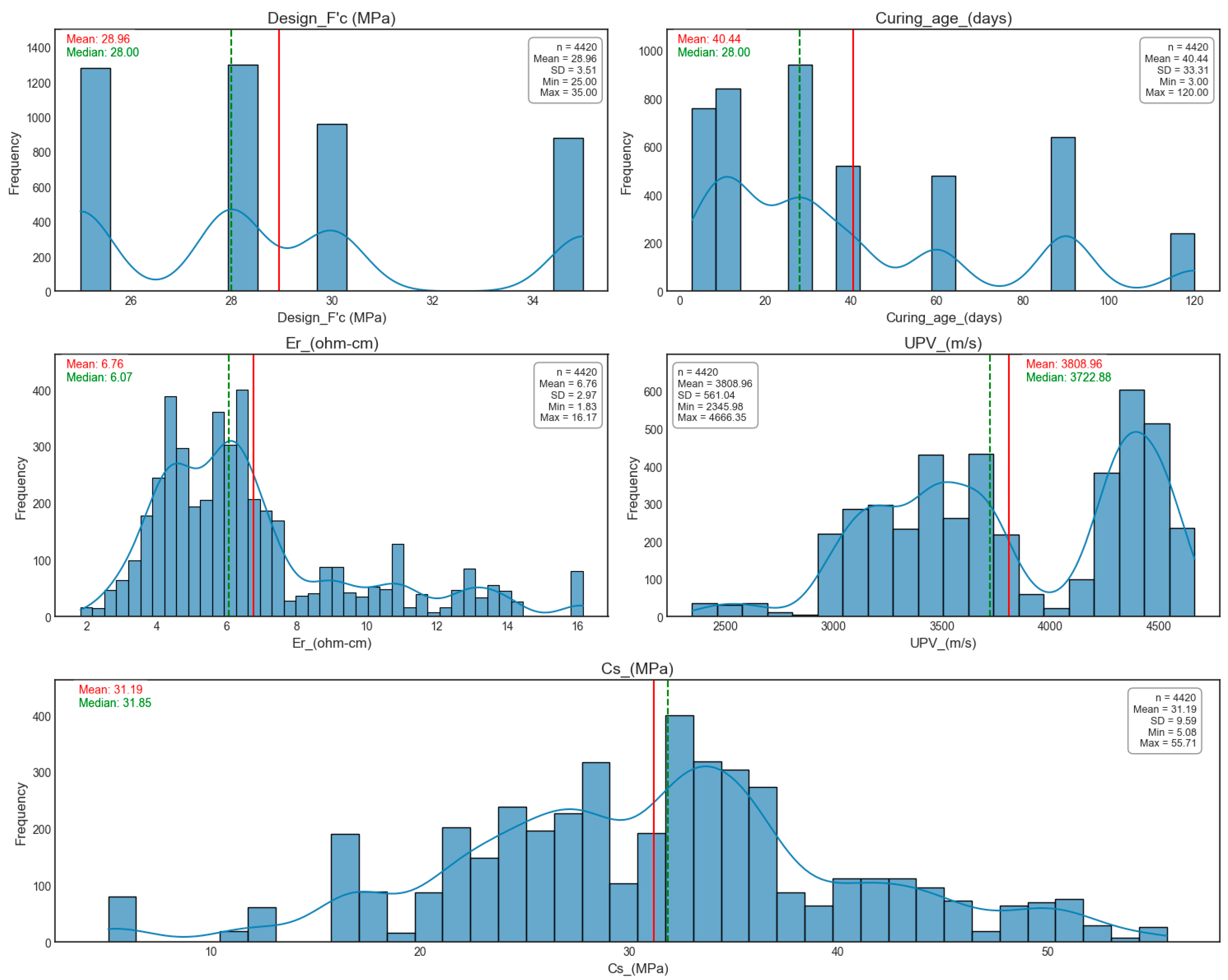
Numerical variables show characteristics typical of concrete engineering applications. Design_F′c has a moderate mean of 28.96 MPa (SD = 3.51) with moderate positive skewness (0.60) and a range of 25.0–35.0 MPa. Curing_age exhibits high variability, averaging 40.44 days (SD = 33.31), ranging from 3–120 days with moderate positive skewness (0.94). Er shows a mean of 6.76 Ω·cm and pronounced skewness (1.25), reflecting concentration at lower resistivity values. UPV displays near-symmetry (Skewness = −0.17) around its mean of 3808.96 m/s. The target variable, Cs, exhibits excellent balance with minimal skewness (−0.03) with a mean compressive strength of 31.19 MPa and substantial variability (5.08–55.71 MPa), confirming dataset suitability for regression modeling.

2.1.2. Feature–Target Relationship Analysis

Table 2. Statistical significance and effect size analysis for feature–target relationships.

Feature	Type	Parametric Test	Non-Parametric Test	p-Value	Effect Size	Significance
Type of cement	Categorical	ANOVA F = 2850.53	K-W H = 2973.80	<0.001	η2 = 0.659	***
Brand	Categorical	ANOVA F = 3174.47	K-W H = 1742.10	<0.001	η2 = 0.418	***
Additives	Categorical	ANOVA F = 1450.97	K-W H = 2277.61	<0.001	η2 = 0.568	***
Type of aggregates	Categorical	ANOVA F = 1518.28	K-W H = 2354.88	<0.001	η2 = 0.508	***
Design_F′c	Numerical	Pearson r = 0.7902	Spearman r = 0.80	<0.001	r2 = 0.624	***
Curing_age	Numerical	Pearson r = 0.7443	Spearman r = 0.80	<0.001	r2 = 0.554	***
Er	Numerical	Pearson r = 0.6813	Spearman r = 0.73	<0.001	r2 = 0.464	***
UPV	Numerical	Pearson r = 0.5610	Spearman r = 0.56	<0.001	r2 = 0.315	***

Note: For categorical variables, the ANOVA F-statistic and Kruskal–Wallis H-statistic are reported. For numerical variables, Pearson and Spearman correlation coefficients with Cs are provided. Effect size is represented as η² (Eta-squared) for categorical variables and r² for numerical variables. Higher values indicate stronger relationships with the target variable. Significance codes: *** p < 0.001.

systematically evaluates statistical significance and strength of relationships between each feature and the target variable, Cs, employing both parametric and non-parametric tests to ensure robust relationship assessment.

All investigated relationships demonstrate high statistical significance (p < 0.001), confirming the relevance of each feature for modeling concrete strength. Among categorical variables, Type of cement exhibits the strongest effect (η² = 0.659), underscoring its substantial role in strength optimization. Additives show robust effects (η² = 0.568), emphasizing chemical additions’ critical contribution to enhancing binding properties and durability. Type of aggregates also exerts a strong influence (η² = 0.508), confirming the relevance of aggregate gradation and mineral composition on mechanical integrity. Brand shows notable impact (η² = 0.418), reflecting manufacturing practices’ importance in cement performance consistency.

Among numerical variables, Design_F′c correlates most strongly with compressive strength (r² = 0.624), aligning with its role as a direct strength design parameter. Curing_age shows high influence (r² = 0.554), validating prolonged hydration time as a driver of crystalline microstructure development in concrete. Er demonstrates a strong correlation (r² = 0.464), reflecting its sensitivity to pore structure and chloride ingress resistance, which are indirect markers of long-term durability. UPV exhibits a moderate but significant correlation (r² = 0.315), supporting its utility in NDE by linking wave propagation speed to internal crack density and homogeneity.

2.1.3. Exploratory Data Visualization

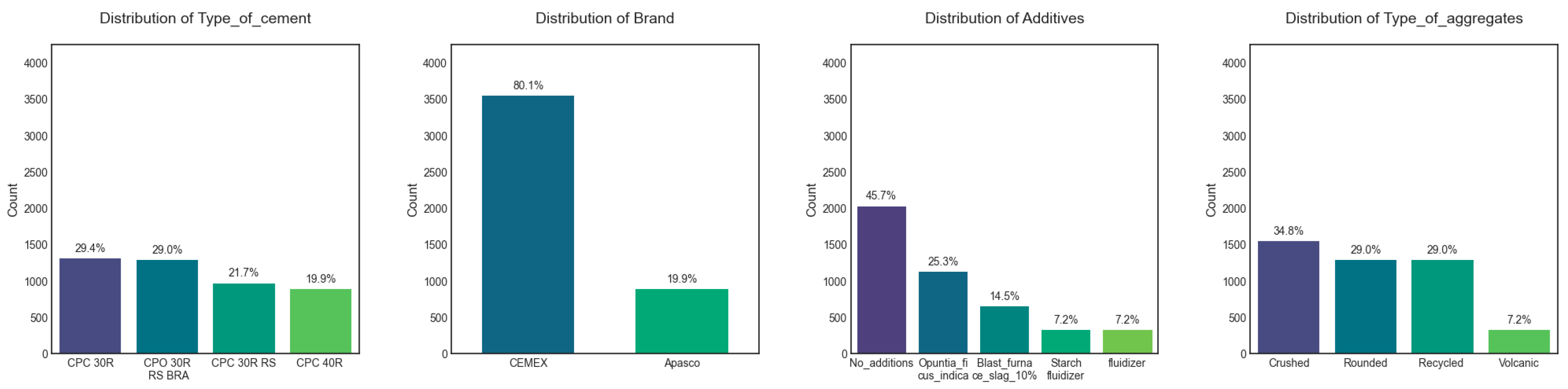
Figure 2 and Figure 3 present a comprehensive visualization of categorical and numerical variable distributions, providing visual insights into dataset characteristics and informing subsequent modeling decisions. The Type of cement variable is relatively balanced across its four categories, while the Brand variable is dominated by “CEMEX”. Among numerical variables, Cs spans a broad range (5–55 MPa), underscoring the dataset diversity.

Figure 2 shows that categorical variables exhibit distinct frequency distributions. Type of cement is fairly balanced across four categories, each representing approximately one-quarter of the samples. In contrast, Brand shows a strong predominance of “CEMEX” (80.1%), with the remaining 19.9% classified as “Apasco.” For Additives, 45.7% of samples are labeled “No additions,” followed by “Opuntia_ficus_indica” (25.3%), “Blast_furnace_slag_10%” (14.5%), “Starch_fluidizer” (7.2%), and “Fluidizer” (7.2%). Similar variability is observed in the distribution for Type of aggregates.

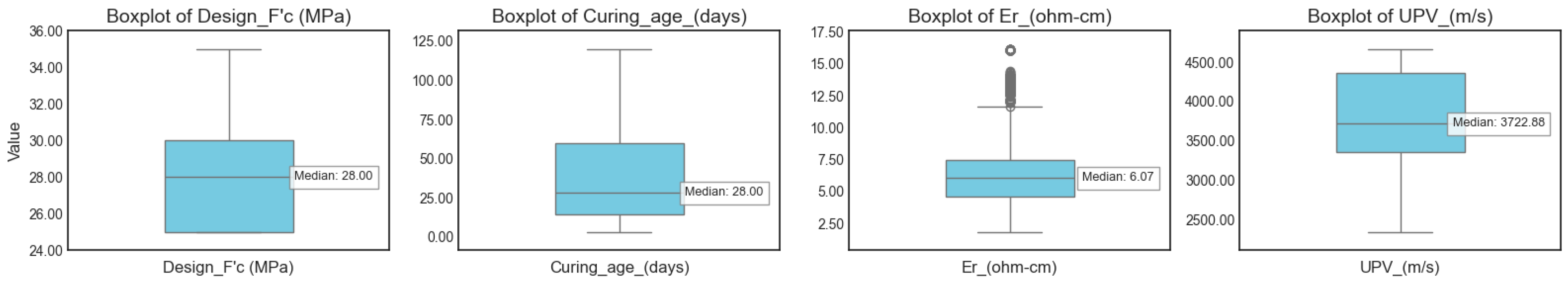
Figure 3 displays histograms of numerical variables, highlighting their key statistical properties. Design_F′c clusters around multiple peaks (e.g., 25, 28, 30, and 35 MPa), reflecting diverse mix design targets. Curing_age has a mean of nearly 40 days but is right-skewed due to significant samples cured for extended periods. Er has a mean of approximately 6.76 Ω·cm, with outliers at higher values. UPV shows a skewed distribution, averaging around 3809 m/s. The target variable, Cs, spans values, emphasizing dataset diversity.

2.1.4. Feature–Target Visual Analysis

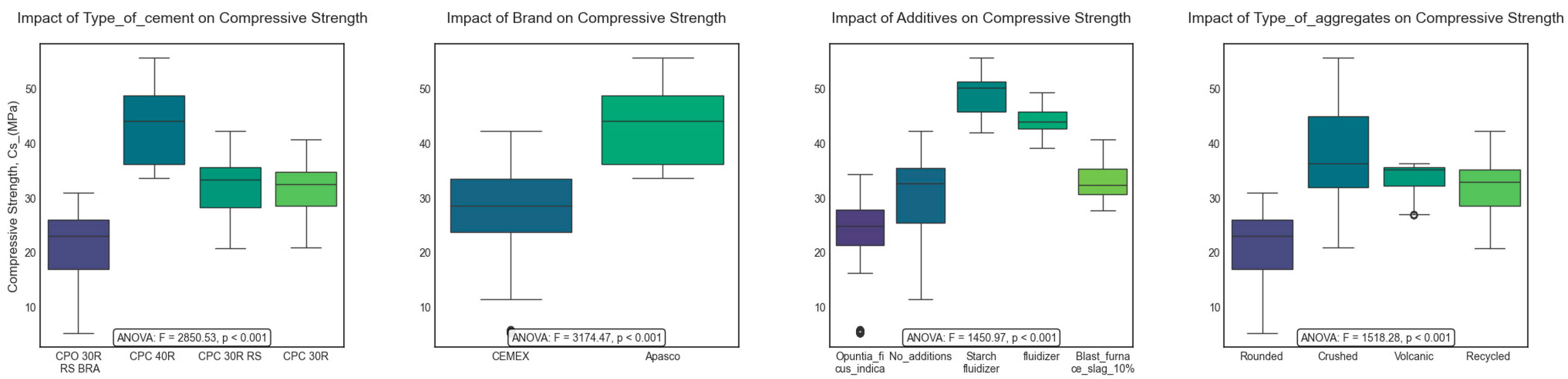
Figure 4 and Figure 5 illustrate quantitative relationships between features and compressive strength through systematic boxplot analysis, revealing the impact of categorical and numerical variables on strength development patterns. Figure 4 demonstrates distinct patterns across categorical variables: Type of cement exhibits a clear impact, with certain varieties showing higher median strengths and narrower interquartile ranges, suggesting consistent performance. Brand reveals systematic differences in strength distributions between manufacturers, reflecting variations in production quality or material composition. Additives cause distinct mechanical performance variations via microstructural modifications in the composite material. Type of aggregates significantly influences structural integrity, with different geometries and material properties leading to divergent performance outcomes.

For numeric features (Figure 5), Design_F′c, conceptually tied to nominal strength class, shows a median of nearly 29 MPa but displays noticeable variability, indicating deviations from theoretical expectations. Curing_age spans 7 to over 100 days, emphasizing the critical role of prolonged hydration in achieving target mechanical properties. Er varies widely across the dataset, with notable outliers linked to environmental or compositional anomalies. UPV exhibits significant variation and outliers, which may stem from specialized admixtures or inconsistencies in testing protocols. These observations collectively highlight how material choices, design parameters, and testing conditions shape compressive strength variability in concrete composites.

2.2. Data Preprocessing

2.2.1. Data Splitting and Stratification

The dataset was divided into three subsets using stratified sampling to maintain representative distributions across all strength ranges. The training set (70%; n = 3094) enables comprehensive model training and feature engineering optimization. The validation set (10%; n = 442) supports hyperparameter tuning and architecture selection without data leakage. The testing set (20%; n = 884) provides an unbiased final performance evaluation.

Stratified sampling maintains a consistent target variable (Cs) distribution across all subsets, preventing bias toward specific strength ranges and maintaining statistical representativeness. This approach enables reliable model comparison and robust generalization assessment across diverse concrete applications.

2.2.2. Data Quality Assessment

Comprehensive data quality verification ensures dataset integrity and identifies potential preprocessing requirements. Missing value detection using automated algorithms and manual inspection confirmed zero missing entries across all 4420 samples (Table 1), eliminating imputation requirements and maintaining complete data integrity.

Data consistency verification across categorical and numerical variables revealed appropriate value ranges and logical distributions. Categorical variables showed balanced representation without inappropriate categories, while numerical parameters remained within expected engineering ranges.

2.2.3. Feature Encoding and Transformation

Systematic feature transformation ensures optimal ML compatibility while preserving engineering interpretability. Categorical variables (Type of cement, Brand, Additives, Type of aggregates) underwent one-hot encoding to generate binary representations, avoiding artificial ordinality assumptions and ensuring proper algorithmic interpretation.

Numerical features (Design_F′c, Curing_age, Er, UPV) retained original scales to preserve engineering relevance while enabling polynomial feature generation. The preprocessing pipeline implementation follows a structured sequence: numerical polynomial expansion, categorical encoding, and horizontal concatenation into a unified feature matrix.

Implementation employs scikit-learn’s PolynomialFeatures (degree = 2, include_bias = False) for numerical expansion and OneHotEncoder (sparse_output = False, handle_unknown = ‘ignore’) for categorical transformation. Stratified sampling for train-validation-test splits (70%-10%-20%) uses the target variable (Cs) to maintain representative strength distributions across all subsets.

This systematic approach maintains complete traceability to original variables for interpretability analysis while ensuring algorithmic compatibility. The preprocessing pipeline generates 15 categorical binary features through one-hot encoding of the four categorical variables (Type of cement: four categories, Brand: two categories, Additives: five categories, Type of aggregates: four categories), which, combined with 14 polynomial numerical features, creates the final 29-dimensional feature space. The methodology balances informational fidelity with technical requirements, maximizing predictive potential without distorting inherent feature relationships.

2.3. Polynomial Feature Engineering

Polynomial feature engineering transforms raw measurements into expanded representations that systematically capture nonlinear relationships governing concrete strength development, enabling subsequent physics-consistent interpretation through feature importance analysis. The correlation patterns resulting from this approach are illustrated in Figure 6. Given the numerical feature vector x = [Design_F′c, Curing_age, Er, UPV], as defined in Table 1, degree-2 polynomial expansion systematically generates 14 polynomial terms, as expressed in Equation (1):

$$P\left(x\right)=\{x_1,x_2,x_3,x_4,x_1^2,x_2^2,x_3^2,x_4^2,x_1{x}_2,x_1{x}_3,x_1{x}_4,x_2{x}_3,x_2{x}_4,x_3{x}_4\}$$

(1)

where x₁ = Design_F′c, x₂ = Curing_age, x₃ = Er, and x₄ = UPV. This expansion enables systematic capture of linear effects, quadratic effects, and interaction effects without pre-selecting specific feature combinations based on theoretical assumptions.

Unlike true physics-informed approaches that embed domain knowledge directly into model architecture, this methodology employs polynomial expansion, followed by post hoc physics-consistent validation through interpretability analysis. This approach ensures objective feature discovery while maintaining alignment with established concrete science principles.

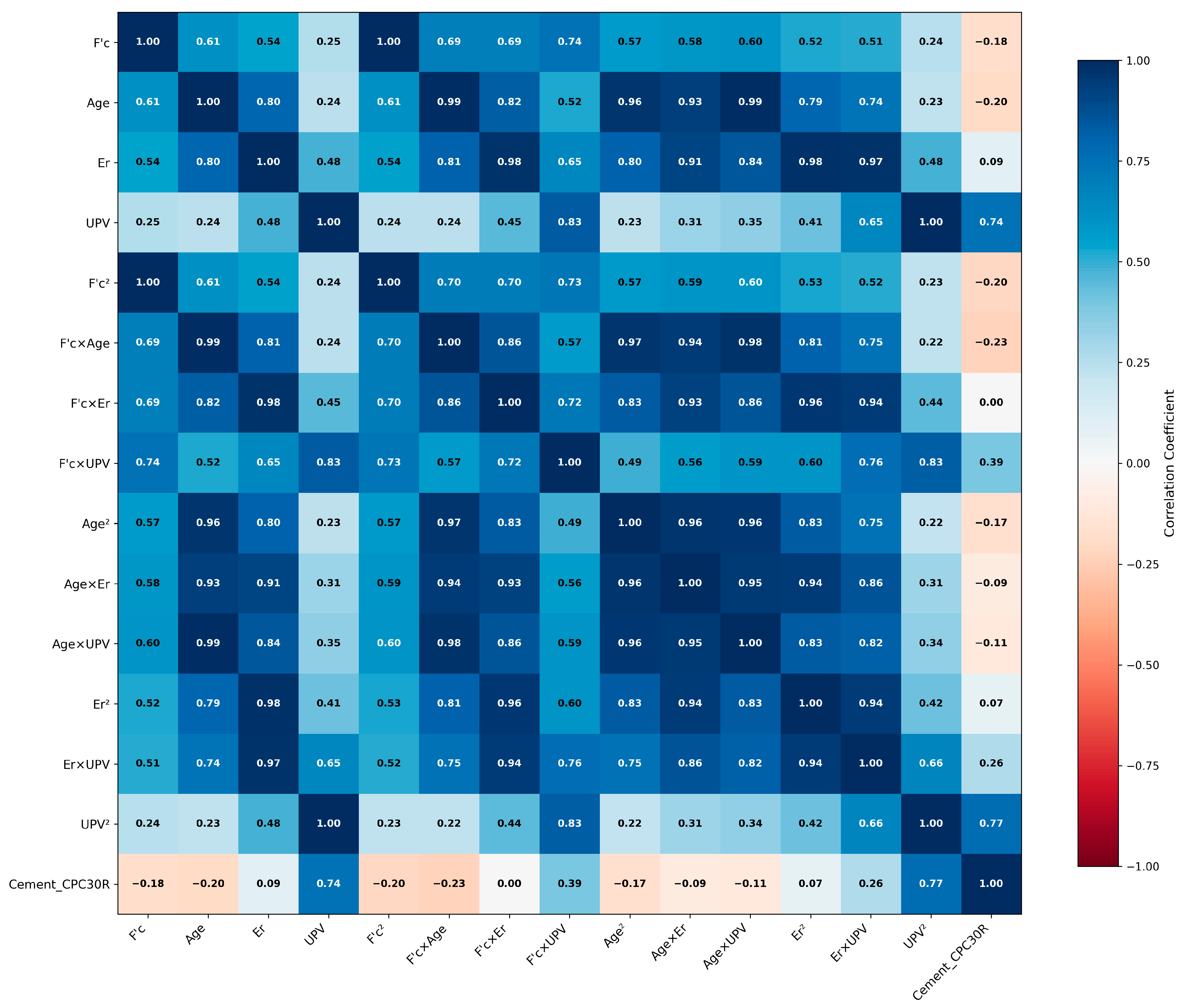
The 14 polynomial terms are combined with 15 categorical binary features (generated through one-hot encoding) to create the complete 29-dimensional feature matrix for model training. Correlation analysis of the original four numerical features reveals moderate intercorrelations: Design_F′c with Curing_age (r = 0.61), Curing_age with Er (r = 0.80), Er with Design_F′c (r = 0.54), and UPV showing weaker correlations (r = 0.24–0.48). All original feature correlations remain below the critical threshold of 0.9, confirming appropriate multicollinearity management.

Figure 6 presents the correlation matrix of the top 15 most important features, demonstrating the systematic correlation patterns resulting from polynomial expansion. This methodology creates expected correlations among derived features (25 pairs with |r| > 0.9), which are mathematically inherent: quadratic terms naturally correlate with their linear counterparts (e.g., Design_F′c vs. Design_F′c²: r = 1.00), while interaction terms exhibit strong relationships with constituent features.

Rather than eliminating correlated features, the ensemble learning approach inherently handles multicollinearity through feature subsampling and regularization while maintaining the rich feature space necessary for capturing complex concrete behavior. This approach aligns with established practices in materials science where polynomial expansions are used to model complex physical phenomena, and multicollinearity among derived features is expected and beneficial for capturing system behavior.

SHAP analysis identifies which generated features contribute most significantly to model predictions, providing objective feature importance assessment without confirmation bias while validating that the most important features are interaction terms reflecting concrete physics principles.

2.4. Model Development

Model development integrated polynomial feature engineering, ensemble learning, and systematic optimization frameworks. All experiments used Python 3.10.13 with scikit-learn 1.3.2, pandas 2.0.3, and NumPy 1.24.3 on a Windows 10 workstation (Intel i7-4770, 16 GB RAM).

Reproducibility was ensured through comprehensive random seed management with random_state = 42 applied consistently across data splitting, model initialization, cross-validation procedures, and hyperparameter optimization processes.

Model-specific preprocessing involved selective application of StandardScaler normalization exclusively to neural networks and support vector machines for optimal convergence, while tree-based ensemble methods utilized raw preprocessed features to preserve interpretability and leverage their inherent scale robustness.

2.4.1. Baseline Architecture

Seven state-of-the-art algorithms were implemented (with the AdaBoost methodology detailed in Algorithm 1), representing diverse ML paradigms spanning interpretability levels from highly interpretable to complex. Traditional methods include linear regression using ordinary least squares, providing interpretable baseline performance, and AdaBoost regression, implementing sequential ensemble learning with decision tree base learners. Advanced ensemble methods comprise Random Forest using parallel ensemble with bootstrap aggregation, XGBoost implementing gradient boosting with advanced regularization techniques, and LightGBM providing efficient gradient boosting with histogram-based optimization. Neural and kernel approaches encompass neural networks using multi-layer perceptrons with adaptive learning capabilities, and support vector regression employing kernel-based regression with Radial Basis Function (RBF) kernel.

To ensure fair comparison across all baseline methods, systematic hyperparameter optimization was applied to all models except linear regression, which uses deterministic ordinary least squares requiring no optimization. Bayesian optimization using BayesSearchCV was employed for ensemble methods with search spaces derived from the established literature and domain expertise, while Grid search optimization was applied to the neural network and support vector regression. The optimization process evaluated 50–100 parameter combinations per model using five-fold cross-validation with negative mean squared error as the scoring metric. Complete optimization specifications, parameter ranges, and theoretical justifications are provided in Appendix A (

Table A1. Comprehensive hyperparameter optimization specifications for baseline models.

Model	Parameter	Range	Justification	Best Parameters
AdaBoost Regression	n_estimators	[50, 200]	Sequential learner optimization	70
	learning_rate	[0.1, 1.5]	Weak learner contribution	1.5
	max_depth	[3, 9]	Base learner complexity	7
	min_samples_split	[2, 10]	Split significance	3
	min_samples_leaf	[1, 5]	Leaf node constraints	1
Random Forest	n_estimators	[50, 200]	Bias–variance balance	180
	max_depth	[5, 20]	Complexity management	16
	min_samples_split	[2, 10]	Statistical significance	10
	min_samples_leaf	[1, 5]	Terminal node reliability	1
XGBoost	n_estimators	[50, 200]	Ensemble size optimization	138
	learning_rate	[0.01, 0.3]	Convergence control	0.043
	max_depth	[3, 10]	Tree complexity	7
	subsample	[0.6, 1.0]	Regularization through sampling	0.879
	colsample_bytree	[0.6, 1.0]	Feature sampling regularization	0.914
LightGBM	n_estimators	[50, 200]	Ensemble optimization	142
	learning_rate	[0.01, 0.3]	Gradient step control	0.198
	max_depth	[3, 15]	Tree depth management	6
	num_leaves	[10, 100]	Leaf complexity control	100
	subsample	[0.6, 1.0]	Sample regularization	0.773
Neural Network	hidden_layer_sizes	[(50,), (100,), (100,50), (150,)]	Architecture exploration	(100,50)
	alpha	[0.0001, 0.001, 0.01]	L2 regularization strength	0.01
	learning_rate_init	[0.001, 0.01, 0.1]	Initial learning rate	0.001
Support Vector Regression	C	[0.1, 1, 10, 100]	Regularization parameter	C = 100
	gamma	[‘scale’, ‘auto’, 0.001, 0.01]	RBF kernel parameter	‘scale’
	epsilon	[0.01, 0.1, 0.2]	Error tolerance	0.2

), ensuring methodological transparency and reproducibility.

2.4.2. PolyBayes-ABR Framework

The PolyBayes-ABR model (as outlined in Algorithm 2) integrates three key components: polynomial feature integration for nonlinear relationship capture, AdaBoost ensemble framework providing robust learning through iterative refinement, and systematic hyperparameter optimization applied consistently across all methods. The AdaBoost algorithm implements iterative learning where base learners h_i are decision trees and weights α_i emphasize difficult training instances according to Equation (2):

$$H\left(x\right)={\sum }_i{\alpha }_i{h}_i\left(x\right)$$

(2)

Algorithm 1 AdaBoost Regression (ABR Model)

1: procedure BasicAdaBoostRegression(X_train, y_train, X_test) 2:  base_estimator ← DecisionTreeRegressor(max_depth = 7) 3:  model ← AdaBoostRegressor(estimator = base_estimator, n_estimators = 70, learning_rate = 1.5) 4:  model.fit(X_train, y_train) 5:  predictions ← model.predict(X_test) 6:  return model, predictions 7: end procedure

Algorithm 2 Polynomial AdaBoost Regression with Bayesian Optimization (PolyBayes-ABR Model)

1: procedure PolyBayes-ABR(X_train, y_train, X_val, y_val, X_test, y_test) 2:  X_num ← numeric_features, X_cat ← categorical_features 3:  poly ← PolynomialFeatures(degree = 2, include_bias = False) 4:  X_train_poly ← poly.fit_transform(X_train_num) 5:  if X_cat exists then 6:    encoder ← OneHotEncoder(sparse_output = False) 7:    X_train_cat ← encoder.fit_transform(X_train_cat) 8:    X_train_final ← concatenate(X_train_poly, X_train_cat) 9:  else 10:    X_train_final ← X_train_poly 11:  end if 12:  //Same transformations applied to X_val and X_test 13:  base_estimator ← DecisionTreeRegressor(random_state = 42) 14:  model ← AdaBoostRegressor(estimator = base_estimator) 15:  param_space ← {n_estimators: [50, 200], learning_rate: [0.1, 1.5], max_depth: [3, 9], 16:    min_samples_split: [2, 10], min_samples_leaf: [1, 5]} 17:  best_params ← BayesSearchCV(model, param_space).fit(X_train_final, y_train) 18:  best_model ← AdaBoostRegressor with best_params 19:  best_model.fit(X_train_final, y_train) 20:  return best_model, metrics, feature_importance 21: end procedure

2.4.3. Hyperparameter Optimization Framework

Hyperparameter optimization uses domain-informed search ranges based on ensemble learning theory to ensure systematic parameter exploration.

Table 3. Hyperparameter search space configuration.

Parameter	Range	Justification
n_estimators	[50, 200]	Bias–variance trade-off optimization
learning_rate	[0.1, 1.5]	Convergence speed vs. overfitting prevention
max_depth	[3, 9]	Interaction complexity management
min_samples_split	[2, 10]	Statistical significance of splits
min_samples_leaf	[1, 5]	Terminal node reliability

presents the comprehensive hyperparameter search space configuration with theoretical justifications for each parameter range.

Bayesian optimization with Gaussian process modeling explores the hyperparameter space defined in Table 3. The optimization used five-fold cross-validation with negative mean squared error as the scoring metric to evaluate each parameter combination during the search process. The domain-informed ranges balance model complexity with computational efficiency while avoiding regions known to produce suboptimal performance.

2.5. Performance Evaluation Framework

2.5.1. Statistical Metrics

Five complementary regression metrics provide performance assessment [37]. Primary metrics include Coefficient of Determination (R²) for evaluating explained variance proportion and Root Mean Square Error (RMSE) for quantifying prediction residual magnitude. Secondary metrics comprise Mean Absolute Error (MAE) for measuring average absolute deviation and Mean Absolute Percentage Error (MAPE) for expressing relative accuracy. The engineering A20 index quantifies predictions within ±20% tolerance, representing industry-standard acceptable accuracy according to structural engineering validation protocols [38]. For model comparisons, R² and RMSE serve as primary performance indicators, while MAE and MAPE provide supplementary error characterization.

2.5.2. Validation Protocol

The evaluation framework uses validation across multiple dimensions to ensure robust performance assessment. A two-stage cross-validation approach is employed: hyperparameter optimization five-fold cross-validation for computational efficiency during parameter selection, while model comparison uses ten-fold cross-validation to ensure robust statistical evaluation across multiple independent data partitions. Statistical significance testing and Cohen’s d analysis provide a comprehensive comparison assessment.

Scenario-based validation across four engineering applications assesses model performance across typical concrete engineering scenarios within the test dataset, including high-strength concrete applications (F′c > 40 MPa), early-age assessment during critical construction periods (Curing_age < 14 days), extended curing for long-term property development (Curing_age > 60 days), and low resistivity conditions (Er < 5 Ω·cm). These scenarios are consistent with established engineering principles for concrete performance and durability [3,4,39]. This approach provides insights into model behavior across diverse concrete characteristics but should be distinguished from true external validation, which would require independent datasets from different sources, time periods, or geographical regions [40,41]. The scenario-based approach represents internal validation across different application domains within the same dataset, providing valuable insights for practical deployment. External validation across independent datasets from different regions and time periods represents a critical future research priority for establishing broader generalizability beyond the current dataset scope.

2.6. SHAP Analysis for Physics-Consistent Interpretability

The SHAP framework provides feature importance assessment through game-theoretic principles, enabling model-agnostic analysis [42]. Implementation employs an automatic explainer selection strategy with fallback mechanisms to ensure analysis across different model types. The analysis prioritizes TreeExplainer for ensemble methods due to computational efficiency and exact SHAP value calculation. When TreeExplainer encounters compatibility issues, the framework automatically transitions to general Explainer with background dataset sampling, and finally to KernelExplainer as the most compatible option.

Implementation conducts analysis on the complete test set (884 instances) rather than random sampling to ensure representative feature importance assessment. Multiple random seeds (42, 123, 456) were tested to verify SHAP value stability across ensemble iterations, confirming consistent interpretability results for the top-ranked features.

The analysis employs post hoc validation to identify physics-meaningful interactions by comparing SHAP-derived feature importance with established concrete materials science principles. Feature importance rankings undergo validation against concrete hydration kinetics, microstructural evolution theory, and transport property relationships to ensure both predictive accuracy and physical interpretability.

The framework implements dual importance assessment comparing SHAP-based importance (mean |SHAP value|) with traditional tree-based feature importance from the AdaBoost model. This comparison provides insights into model behavior and feature utilization patterns. SHAP values demonstrate stability for the top-ranked features across different random seeds, enabling reliable interpretability analysis for engineering applications.

3. Results

This section presents an evaluation of the PolyBayes-ABR framework through systematic comparison with state-of-the-art methods, statistical analysis, and detailed interpretability assessment. Results demonstrate competitive performance while providing physics-consistent insights for concrete engineering applications.

3.1. Performance Comparison

Table 4. Comprehensive model comparison with statistical analysis.

Model	R2 Test	RMSE Test (MPa)	A20 Test (%)	Cross-Val R2 (±SD)	Cross-Val RMSE (±SD)	vs. PolyBayes-ABR (p-Value)	Cohen’s d
Linear Regression	0.9364	2.459	93.55	0.9300 ± 0.0067	2.525 ± 0.090	<0.001 ***	−23.36
AdaBoost	0.9951	0.683	100.00	0.9946 ± 0.0010	0.699 ± 0.060	0.018 *	−0.29
Random Forest	0.9950	0.687	100.00	0.9949 ± 0.0008	0.678 ± 0.060	0.888	0.03
XGBoost	0.9952	0.672	100.00	0.9950 ± 0.0009	0.676 ± 0.060	0.734	0.08
LightGBM	0.9950	0.693	100.00	0.9949 ± 0.0009	0.682 ± 0.065	0.899	−0.03
Neural Network	0.9911	0.921	99.89	0.9919 ± 0.0013	0.860 ± 0.067	<0.001 ***	−2.70
SVR	0.9904	0.955	98.87	0.9903 ± 0.0016	0.938 ± 0.074	<0.001 ***	−3.69
PolyBayes-ABR	0.9957	0.643	100.00	0.9949 ± 0.0009	0.681 ± 0.066	Reference	Reference

Note: Statistical significance: *** p < 0.001, * p < 0.05. All models use optimized hyperparameters for fair comparison.

presents a detailed performance comparison across eight methods representing diverse ML paradigms, from traditional linear approaches to advanced ensemble techniques. The evaluation integrates test set performance, cross-validation robustness, and statistical analysis with effect size assessment. All models except linear regression underwent hyperparameter optimization to ensure fair comparison.

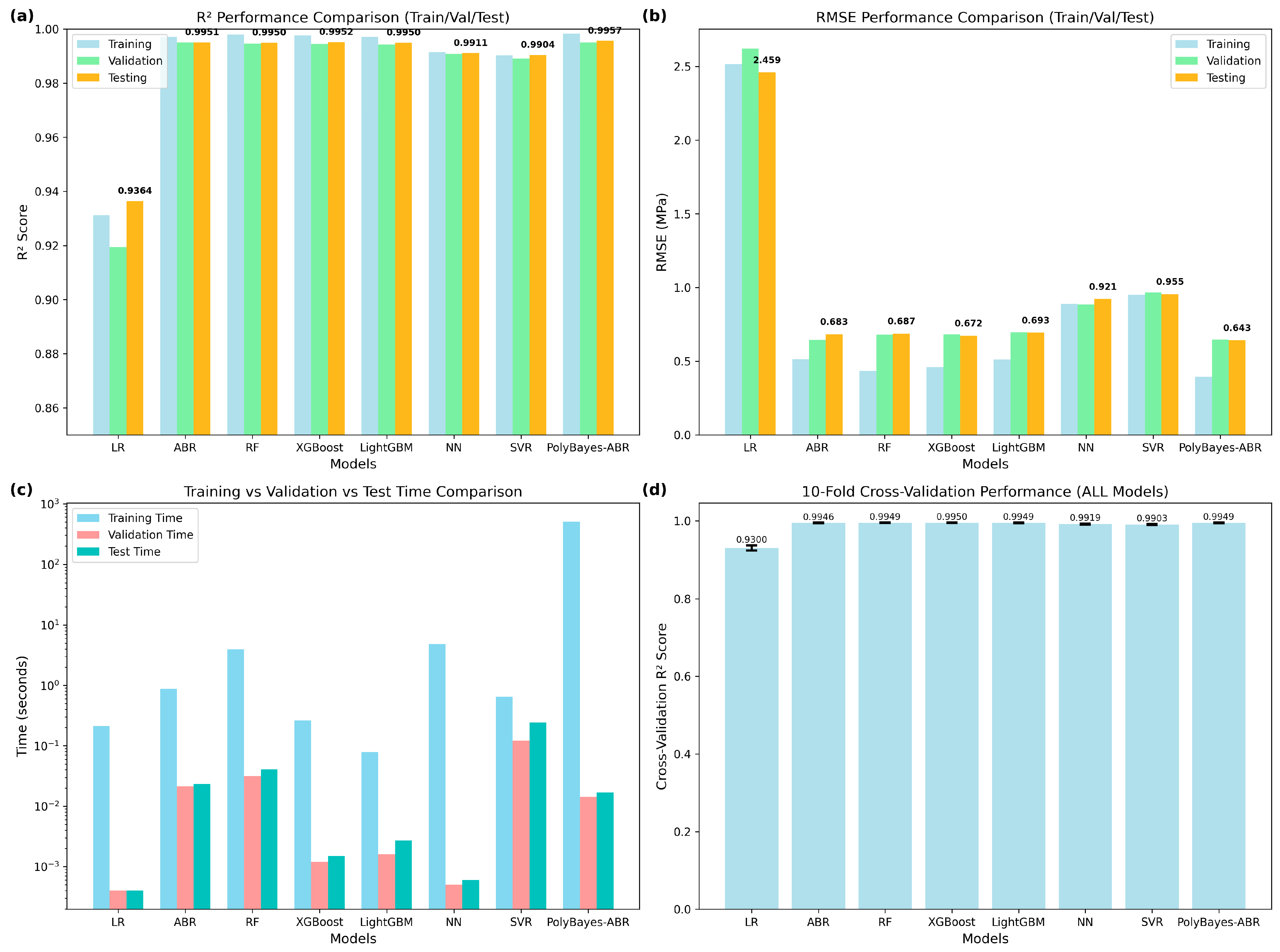
Performance evaluation reveals distinct tiers among the evaluated methods. Traditional approaches, including linear regression, achieve moderate accuracy with R² = 0.9364 and RMSE = 2.459 MPa, with an A20 index of 93.55%. Advanced ensemble methods, including XGBoost, Random Forest, LightGBM, and PolyBayes-ABR, show good performance, with R² values ≥ 0.995 and RMSE values ≤ 0.7 MPa, achieving 100% A20 indices that meet engineering accuracy requirements.

Cross-validation analysis confirms performance consistency across data subsets, with ensemble methods showing low variability (standard deviations ≤ 0.001 for R² and ≤0.070 MPa for RMSE). This consistency indicates good generalization capabilities for deployment on new concrete mixtures.

Statistical testing reveals that PolyBayes-ABR shows comparable performance within the ensemble category, with non-significant differences from XGBoost (p = 0.734), Random Forest (p = 0.888), and LightGBM (p = 0.899), supported by small effect sizes (|Cohen’s d| ≤ 0.08). The analysis shows larger differences from traditional approaches, including linear regression (p < 0.001, Cohen’s d = −23.36), neural networks (p < 0.001, Cohen’s d = −2.70), and SVR (p < 0.001, Cohen’s d = −3.69).

PolyBayes-ABR achieves good performance (R² = 0.9957, RMSE = 0.643 MPa) with statistical equivalence to other ensemble methods. The small performance differences among ensemble methods (RMSE variation ≤ 0.05 MPa) fall within engineering tolerance ranges and measurement uncertainty levels, indicating that accuracy alone cannot justify method selection.

The statistical equivalence among ensemble methods shifts focus from accuracy optimization to practical considerations, including interpretability requirements, uncertainty quantification capabilities, and deployment constraints. When performance differences fall within measurement uncertainty ranges, method selection should prioritize features that enhance engineering decision-making confidence and provide scientific insights into concrete behavior. PolyBayes-ABR offers distinct practical advantages: (1) physics-consistent interpretability through SHAP analysis that aligns with established concrete science principles, (2) enhanced uncertainty quantification with improved prediction intervals (±1.260 MPa vs. ±1.338 MPa baseline), and (3) actionable engineering insights for quality control optimization and mix design improvement that black-box ensemble methods cannot provide.

Based on the detailed performance analysis in

Table A2. Comprehensive performance comparison across state-of-the-art methods.

Model	Dataset	R2	RMSE (MPa)	MAE (MPa)	MAPE (%)	A20 (%)	Time (s)
Linear Regression	Training	0.9312	2.5155	1.9895	7.5867	93.18	0.2132
	Validation	0.9194	2.6217	2.0778	7.8164	92.08	0.0004
	Testing	0.9364	2.4591	1.9461	7.6164	93.55	0.0004
AdaBoost Regression	Training	0.9971	0.5120	0.3848	1.2986	100.00	0.8766
	Validation	0.9951	0.6440	0.4173	1.3483	100.00	0.0214
	Testing	0.9951	0.6835	0.4569	1.5122	100.00	0.0235
Random Forest	Training	0.9979	0.4345	0.2746	0.8957	100.00	3.9565
	Validation	0.9946	0.6806	0.4122	1.3333	100.00	0.0315
	Testing	0.9950	0.6868	0.4180	1.3892	100.00	0.0407
XGBoost	Training	0.9977	0.4595	0.3231	1.0773	100.00	0.2640
	Validation	0.9945	0.6833	0.4156	1.3256	100.00	0.0012
	Testing	0.9952	0.6725	0.4359	1.4357	100.00	0.0015
LightGBM	Training	0.9972	0.5101	0.3449	1.1356	100.00	0.0785
	Validation	0.9943	0.6954	0.4324	1.4217	100.00	0.0016
	Testing	0.9950	0.6928	0.4387	1.4418	100.00	0.0027
Neural Network	Training	0.9914	0.8893	0.6598	2.2408	99.94	4.8568
	Validation	0.9908	0.8838	0.6396	2.1344	100.00	0.0005
	Testing	0.9911	0.9210	0.6650	2.2530	99.89	0.0006
Support Vector Regression	Training	0.9902	0.9502	0.6274	2.5952	98.97	0.6431
	Validation	0.9891	0.9651	0.6468	2.7571	98.64	0.1222
	Testing	0.9904	0.9548	0.6227	2.6909	98.87	0.2434
PolyBayes-ABR	Training	0.9983	0.3956	0.2968	1.0397	100.00	508.8221
	Validation	0.9951	0.6467	0.3930	1.2844	100.00	0.0142
	Testing	0.9957	0.6428	0.4180	1.4073	100.00	0.0169

Note: All baseline models use the full feature set (29 features, including polynomial expansion and categorical encoding). Training times for PolyBayes-ABR include hyperparameter optimization (508.82 s); actual model training time after optimization is ~0.2 s. Validation and test times represent prediction time only. Training time variations reflect feature set complexity and algorithm characteristics.

(Appendix A.2), Figure 7 provides visual evidence supporting these findings across multiple evaluation dimensions, showing consistency in performance metrics across all data splits. Advanced ensemble methods cluster in the high-performance range, while traditional methods exhibit lower accuracy. Computational analysis reveals logarithmic scale differences in training times, from milliseconds for simple methods to optimization processes for advanced approaches.

3.2. Model Performance Analysis

3.2.1. Systematic Ablation Study

Systematic ablation analysis shows individual contributions of polynomial features and hyperparameter optimization to overall performance through a progressive enhancement approach.

Table 5. Comprehensive ablation study results.

Configuration	Description	R2 Test	RMSE Test	Improvement	Training Time
ABR Baseline	Original features, default parameters	0.9225	2.715	-	0.053 s
ABR + Polynomial	Polynomial features, default parameters	0.9419	2.351	ΔR2 = +0.0194	0.186 s
ABR + Optimization	Original features, optimized parameters	0.9878	1.079	ΔR2 = +0.0459	3.591 s
PolyBayes-ABR (Full)	Polynomial features + optimization	0.9957	0.643	ΔR2 = +0.0079	508.822 s

Note: Training times vary by feature set complexity: ABR baseline uses original four features (0.053 s), while subsequent configurations use expanded feature sets (14–29 features). This demonstrates computational impact of feature engineering.

presents detailed ablation results showing progressive improvement from baseline to full implementation.

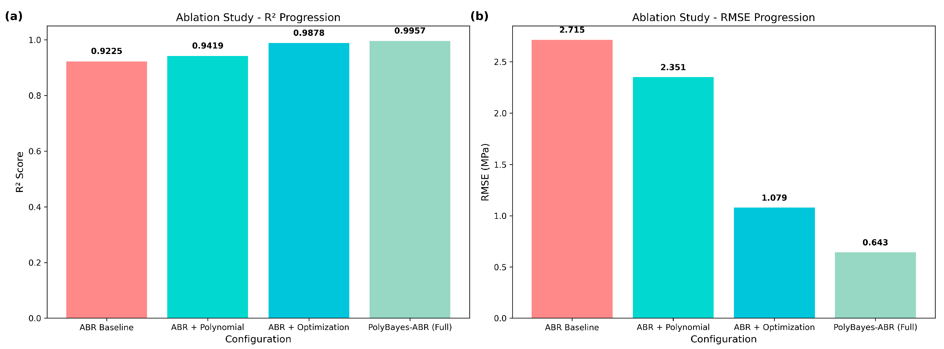
Component analysis reveals insights into the improvement process. The addition of polynomial features improves R² by 0.0194, showing the value of capturing nonlinear relationships in concrete behavior. Hyperparameter optimization provides notable improvement, with R² increasing from 0.9225 to 0.9878 (ΔR² = 0.0653), highlighting the importance of parameter tuning. The combined PolyBayes-ABR approach achieves total improvement of 0.0732 (reaching R² = 0.9957).

The training time increase represents the computational cost of Bayesian optimization. While this appears substantial, it provides practical advantages: (1) improved uncertainty quantification (±1.260 MPa vs. ±1.338 MPa), (2) physics-consistent interpretability through SHAP analysis, and (3) improved accuracy important for safety-critical concrete assessment. The training is performed once during model development, while inference time remains comparable to other methods for deployment.

Figure 8 provides a clear visualization of systematic ablation study results through two complementary perspectives. R² progression panel (left) demonstrates consistent improvement across configuration stages, from ABR Baseline (0.9225) through ABR + Polynomial (0.9419) and ABR + Optimization (0.9878) to the final PolyBayes-ABR (0.9957), illustrating the cumulative benefit of each enhancement. RMSE reduction panel (right) shows corresponding error reduction from 2.715 MPa baseline to 0.643 MPa final performance, with the most substantial improvement occurring through hyperparameter optimization (from 2.351 to 1.079 MPa). The visualization confirms that each component contributes meaningfully to final performance, with synergistic effects exceeding individual contributions, as evidenced by total improvement surpassing the sum of individual enhancements.

3.2.2. Scenario-Based Validation and Robustness Assessment

Scenario-based validation across four engineering applications shows robust performance across different concrete characteristics.

Table 6. Scenario-based validation results across concrete engineering applications.

Scenario	Engineering Rationale	Samples (%)	R2	RMSE (MPa)	MAE (MPa)	MAPE (%)
High-Strength Concrete	High-performance applications (F′c > 40 MPa)	152 (17.2%)	0.935	1.090	0.792	1.698
Early-Age Concrete	Critical curing period (Curing_age < 14 days)	147 (16.6%)	0.998	0.308	0.246	1.589
Extended Curing	Long-term hydration (Curing_age > 60 days)	198 (22.4%)	0.987	0.746	0.449	1.022
Low-Resistivity Concrete	Lower resistivity (Er < 5 Ω·cm)	253 (28.6%)	0.996	0.435	0.325	1.380

Note: Scenarios are overlapping subsets of the 884-sample test set. Percentages indicate the proportion of test samples meeting each condition.

presents detailed performance results across diverse engineering applications, showing the model’s versatility.

Scenario-specific analysis reveals distinct performance characteristics across different concrete applications. High-strength concrete applications (R² = 0.935, RMSE = 1.090 MPa) show acceptable accuracy for structural design applications despite inherent challenges of nonlinear behavior at elevated strength levels. Early-age concrete prediction achieves high accuracy (R² = 0.998, RMSE = 0.308 MPa). Extended curing scenarios show good capability (R² = 0.987, RMSE = 0.746 MPa) for long-term performance prediction. Low resistivity concrete applications achieve strong performance (R² = 0.996, RMSE = 0.435 MPa) despite microstructural complexity.

Overall scenario-based validation shows robust model generalization, with all scenarios maintaining R² > 0.93, indicating that the model captures fundamental relationships that transcend specific mix designs or testing conditions. The achieved accuracy levels meet typical engineering tolerances across different application domains.

3.2.3. Robustness and Uncertainty Analysis

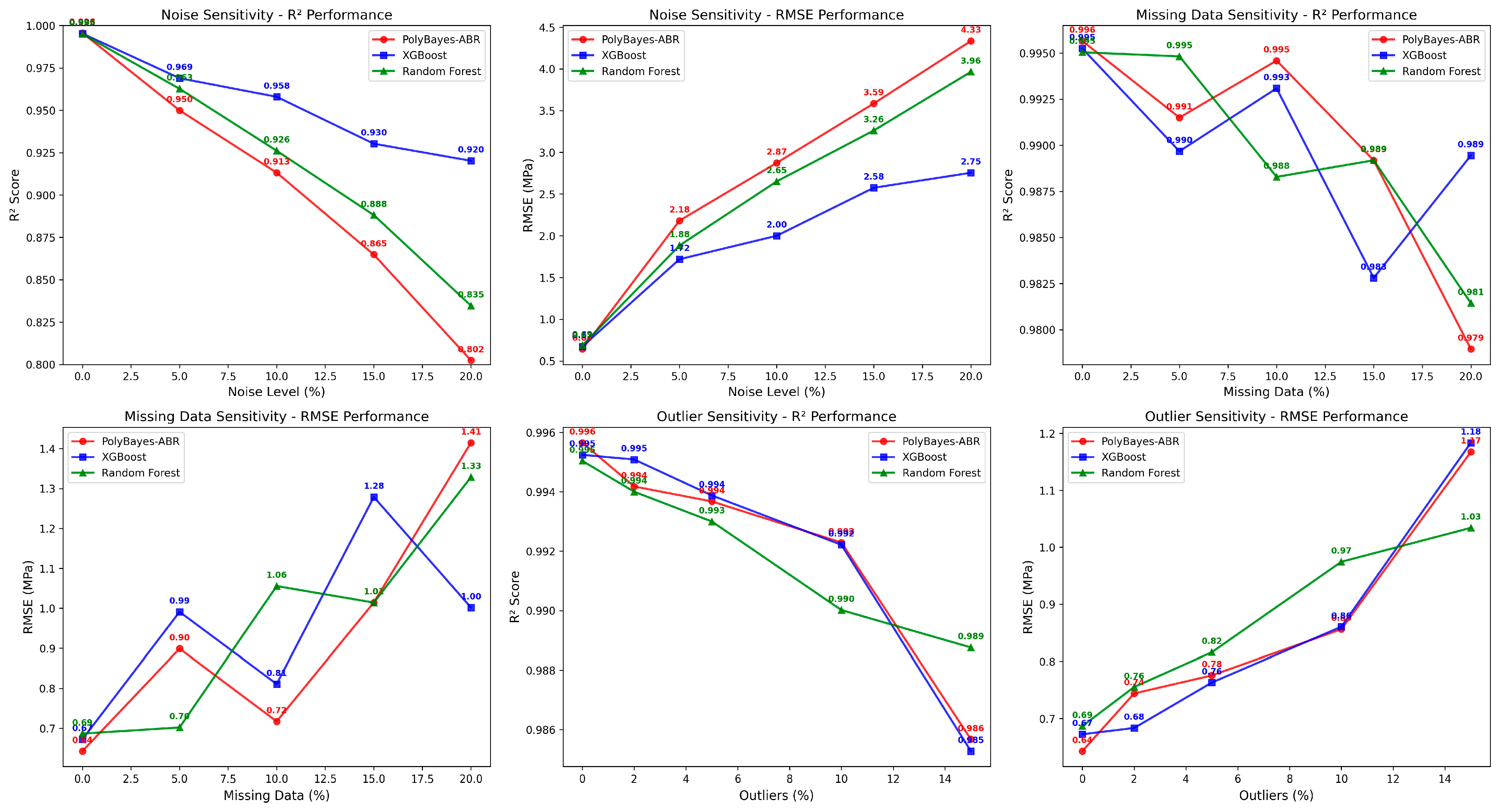
Figure 9 presents a detailed robustness analysis across noise, missing data, and outlier challenges, systematically evaluating model performance under real-world deployment conditions commonly encountered in NDT measurements.

The noise sensitivity evaluation reveals distinct performance characteristics across models under measurement uncertainty conditions. PolyBayes-ABR shows R² degradation of 0.194 (from 0.996 to 0.802) at a 20% noise level, while XGBoost shows better noise tolerance with degradation of 0.075 (from 0.995 to 0.920). Random Forest exhibits intermediate performance with degradation of 0.160 (from 0.995 to 0.835). This indicates that PolyBayes-ABR shows higher sensitivity to measurement noise than ensemble methods.

The missing data evaluation shows good performance across all models. XGBoost shows minimal degradation of 0.006 (from 0.995 to 0.989) at 20% missing data, while PolyBayes-ABR shows low degradation of 0.017 (from 0.996 to 0.979), and Random Forest shows degradation of 0.014 (from 0.995 to 0.981). This resilience to missing data is relevant for field applications where sensor malfunctions or incomplete measurements occur.

Outlier sensitivity evaluation reveals good robustness across all models. PolyBayes-ABR shows minimal degradation of 0.010 (from 0.996 to 0.986) at 15% outlier contamination, with XGBoost showing similar degradation (0.010, from 0.995 to 0.985), and Random Forest showing slightly better robustness (degradation: 0.006, from 0.995 to 0.989).

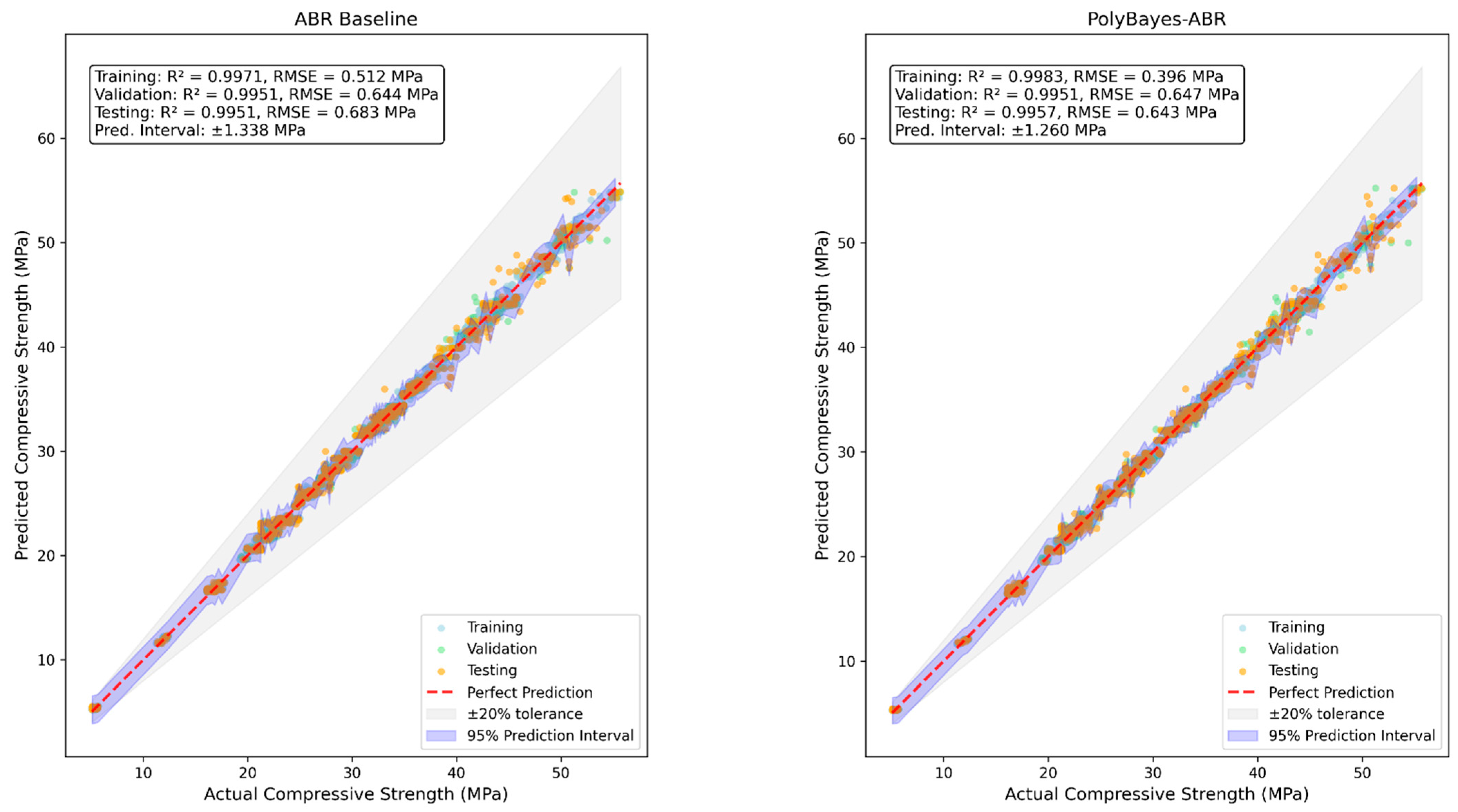
Figure 10 provides detailed prediction accuracy and uncertainty quantification comparison between ABR baseline and PolyBayes-ABR, addressing requirements for safety-critical concrete strength assessment applications.

The comparison shows improvement across evaluation metrics. PolyBayes-ABR achieves prediction intervals of ±1.260 MPa compared to ±1.338 MPa for the baseline, representing a 0.078 MPa (5.8%) reduction in prediction uncertainty. The 95% prediction intervals show consistent uncertainty bounds across the full strength range (5–55 MPa), with both models maintaining predictions within the ±20% engineering tolerance zone.

The combined analysis from Figure 9 and Figure 10 provides an evaluation of model reliability under diverse deployment scenarios. The robustness analysis shows that ensemble methods show better noise tolerance compared to the polynomial expansion approach, while PolyBayes-ABR shows comparable performance under missing data and outlier conditions.

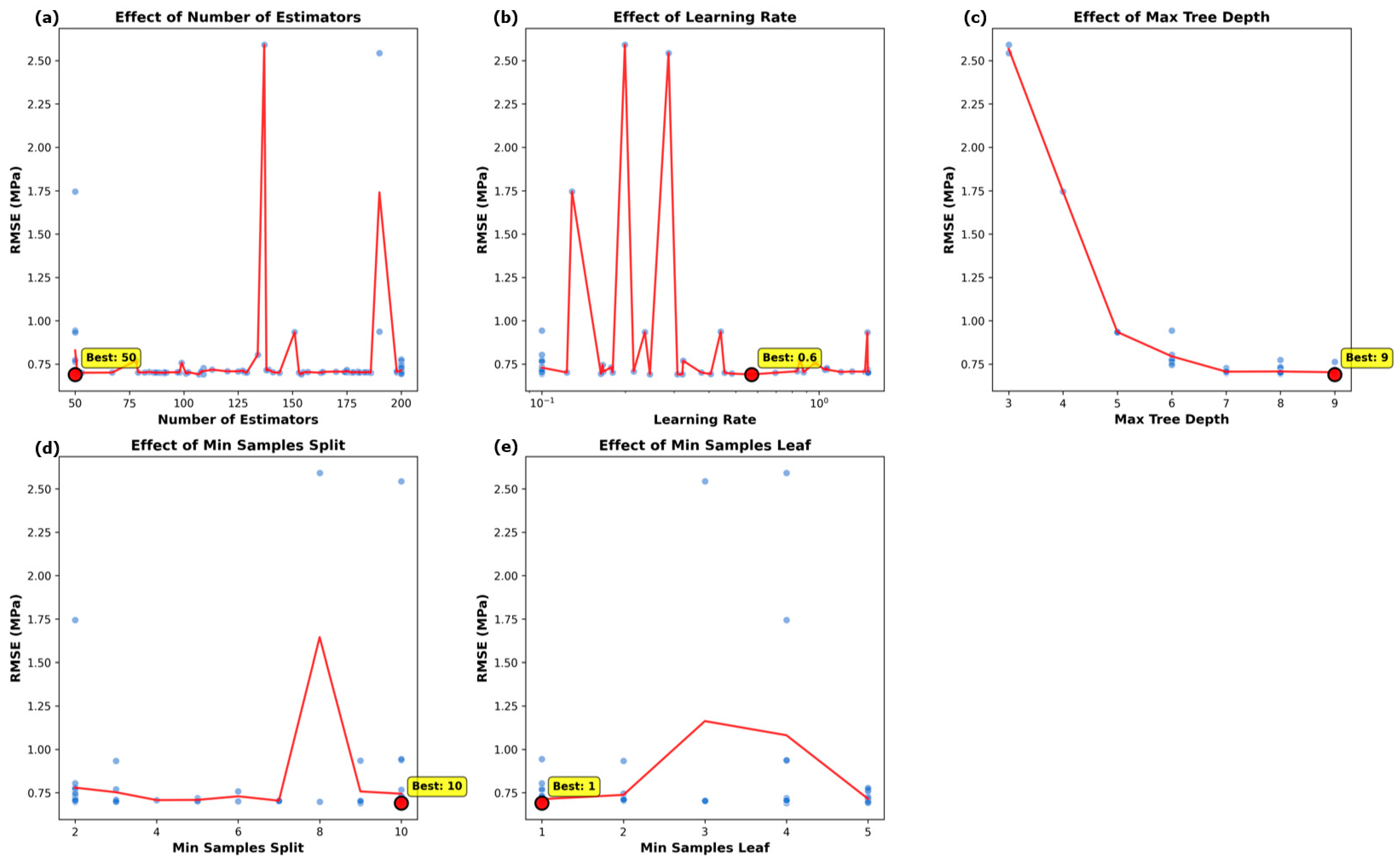
Figure 11 provides a detailed analysis of individual hyperparameter effects through five integrated panels, revealing distinct optimization characteristics for each parameter. The analysis shows that n_estimators achieves optimal performance at 50 estimators, learning_rate shows optimal value at 0.6, max_depth shows optimal performance at 9, min_samples_split exhibits optimal value at 10, and min_samples_leaf shows optimal performance at 1.

Parameter sensitivity analysis reveals distinct optimization characteristics for each hyperparameter. The n_estimators parameter achieves optimal performance at 50 estimators, indicating that moderate ensemble size provides sufficient model complexity without excessive computational overhead. Learning_rate sensitivity shows optimal value at 0.6 with notable performance variations across the range.

Max_depth analysis indicates optimal performance at depth 9, showing that deeper trees can capture complex interactions while maintaining generalization capability. Min_samples_split behavior shows optimal value at 10, indicating that moderate splitting requirements help balance model complexity with fitting capability. Min_samples_leaf analysis shows optimal performance at 1, indicating that flexible leaf creation benefits concrete applications requiring fine-grained decision boundaries to capture material variability.

3.3. Physics-Consistent Feature Analysis

SHAP analysis reveals systematic feature importance patterns that show consistency with established concrete materials science principles. The analysis provides a post hoc interpretability assessment that aligns statistical importance with known concrete behavior relationships, confirming that the polynomial expansion approach captures fundamental material interactions recognized in the concrete engineering literature.

3.3.1. Dual Methodology Assessment

Table 7. Dual feature importance assessment: SHAP and tree-based analysis with physics interpretation and engineering relevance.

Rank	Feature	SHAP Importance	Tree Importance	Physics Interpretation	Engineering Relevance
1	Curing_age × Er	4.2337	0.7577	Hydration-microstructure coupling	Time-dependent densification monitoring
2	Curing_age × UPV	1.4705	0.0527	Porosity evolution tracking	Quality control during curing
3	Design_F′c × Curing_age	1.2342	0.0467	Strength development kinetics	Construction timeline optimization
4	Design_F′c × UPV	0.9457	0.0589	Strength–elastic modulus relationship	Design validation through NDT
5	Type_of_aggregates_Recycled	0.5851	0.0031	Aggregate sustainability effects	Sustainable concrete development
6	Additives_Opuntia_ficus_indica	0.3417	0.0033	Bio-admixture microstructural effects	Green concrete technology
7	UPV	0.2921	0.0077	Direct elastic property measurement	Non-destructive testing applications
8	Additives_No_additions	0.2225	0.0014	Baseline concrete behavior	Reference material characterization
9	UPV2	0.2088	0.0070	Nonlinear elastic behavior	Advanced NDT interpretation
10	Er×UPV	0.1472	0.0089	Transport–mechanical coupling	Multi-property assessment
11	Design_F′c × Er	0.1088	0.0218	Design strength– resistivity correlation	Mix design optimization
12	Type_of_aggregates_Rounded	0.0935	0.0019	Aggregate geometry influence	Material selection guidance
13	Type_of_aggregates_Crushed	0.0907	0.0009	Angular aggregate effects	Mechanical property enhancement
14	Additives_Starch_fluidizer	0.0800	0.0100	Rheological modification effects	Workability optimization
15	Type_of_cement_CPO 30R RS BRA	0.0666	0.0007	Cement composition influence	Material specification guidance

presents detailed feature importance rankings through dual assessment methodology, documenting both SHAP-based importance (mean |SHAP value|) and tree-based feature importance alongside physics interpretation and engineering relevance. This systematic documentation enables evaluation of whether statistical importance aligns with established concrete science principles while providing actionable insights for engineering practice.

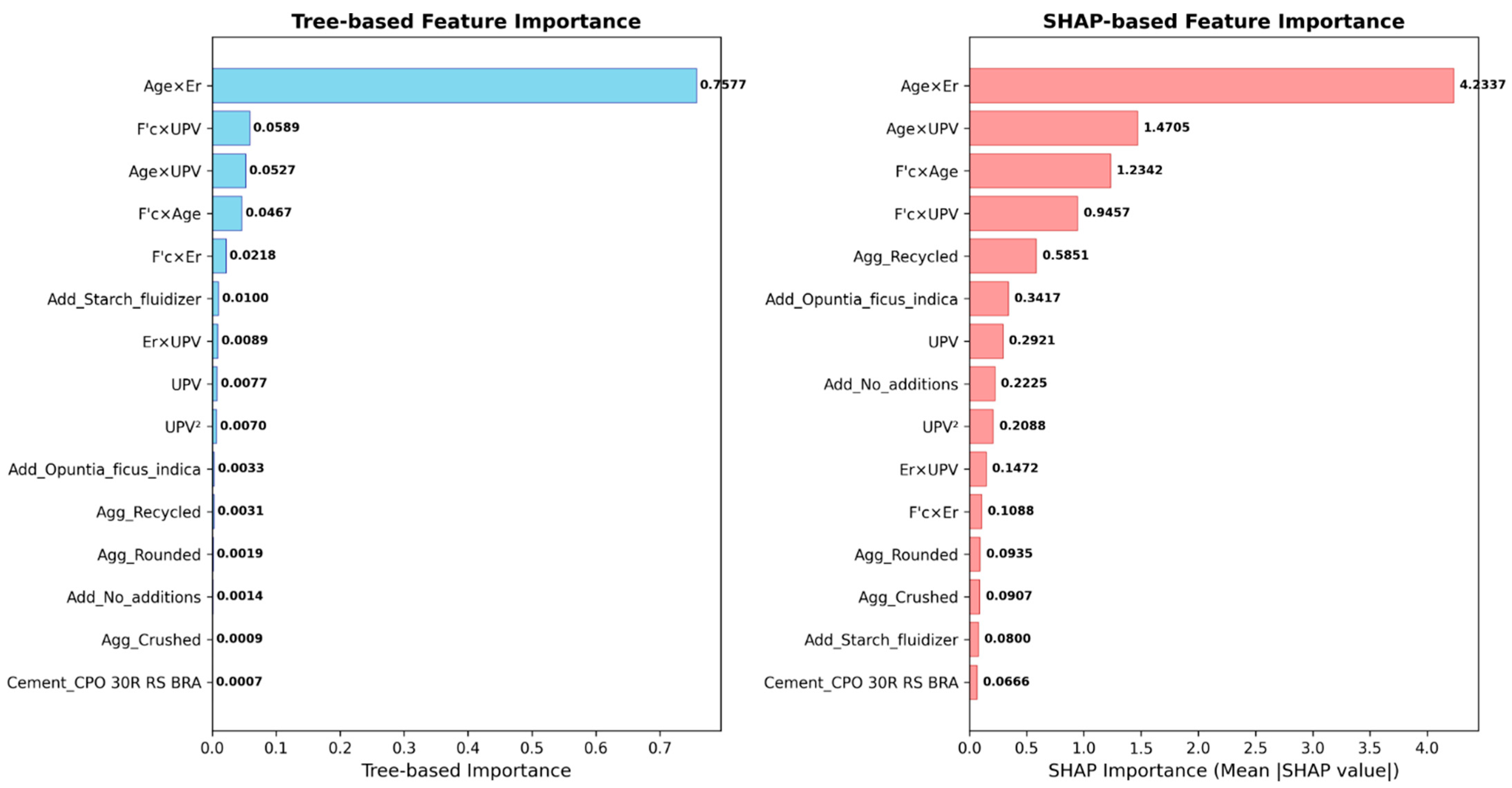
Figure 12 visualizes the magnitude differences between the two importance assessment approaches. The dominant Curing_age × Er interaction achieves SHAP importance of 4.2337 compared to tree importance of 0.7577, representing a 5.59× difference. This pattern shows that SHAP captures feature contributions to prediction accuracy, while tree importance reflects algorithmic feature selection frequency during ensemble training.

The systematic identification of interaction terms in top rankings across both assessments shows consistency with the polynomial expansion approach and supports engineering deployment in applications requiring both accuracy and interpretability.

3.3.2. Physics Consistency Assessment

Quantitative feature importance assessment from Table 7 shows correspondence with established material behavior principles.

Hydration kinetics consistency is represented by the Curing_age × Er interaction (SHAP importance: 4.2337), which aligns with the recognized physics of progressive calcium silicate hydrate (C-S-H) gel formation that creates denser microstructure over time. The relationship between porosity reduction and resistivity increase is consistent with Archie’s law [43], where electrical resistivity reflects microstructural densification during hydration [44].

Mechanical–elastic coupling consistency is captured by Design_F′c × UPV (SHAP importance: 0.9457), aligning with the established relationship between ultrasonic wave propagation and elastic modulus development during cement hydration [45]. UPV serves as an indicator of elastic properties and internal structure quality.

Strength development kinetics consistency is represented by Design_F′c × Curing_age (SHAP importance: 1.2342), which aligns with the principle that target strength achievement requires adequate hydration time. This time-dependent relationship shows that higher design strengths typically require proportionally longer curing periods.

Transport-mechanical coupling consistency is characterized by Er × UPV (SHAP importance: 0.1472), reflecting the principle that porosity reduction during hydration affects both electrical conductivity and mechanical wave propagation simultaneously.

3.3.3. Engineering Implementation Framework

Engineering relevance assessment in Table 7 translates statistical findings into practical applications. Quality control applications emerge from the dominant interaction terms, with Curing_age × Er enabling time-dependent densification monitoring protocols and Curing_age × UPV supporting quality control during curing phases.

Mix design optimization benefits from the identified Design_F′c interactions with both Curing_age and UPV measurements. The systematic ranking of aggregate and additive effects provides material selection guidance for sustainable concrete development and green concrete technology implementation.

NDT strategy development is supported by the multiple UPV-related interactions identified in Table 7, ranging from direct elastic property measurement to advanced interpretation of nonlinear elastic behavior.

3.3.4. Model Validation Through Physics Consistency

Feature importance analysis from Table 7 reveals that interaction terms dominate the top-ranking features, with the highest-ranked features showing substantially higher importance than individual material properties. This pattern shows consistency with the nonlinear, synergistic nature of concrete behavior that cannot be adequately captured through linear relationships alone.

The correspondence between high feature importance rankings and established concrete science principles suggests that the ML model has successfully captured physically meaningful relationships rather than spurious correlations. This physics consistency, shown through both quantitative rankings (Table 7) and visual evidence (Figure 12), provides confidence in the model’s applicability for engineering decision-making processes in safety-critical concrete applications.

4. Discussion

This section interprets the evaluation results and discusses their implications for concrete engineering practice. The analysis addresses methodological contributions, practical implementation considerations, and identifies directions for future research based on the comprehensive evaluation presented in Section 3.

4.1. Methodological Contributions and Implications

4.1.1. Interpretability Framework Assessment

The PolyBayes-ABR framework represents a post hoc interpretability approach rather than true physics-informed machine learning. This distinction is important: while physics-informed ML embeds domain knowledge directly into model architecture [46], this methodology employs systematic polynomial expansion followed by physics-consistent validation through SHAP analysis.

This approach offers specific advantages for concrete engineering: feature discovery through systematic polynomial expansion of numerical variables, exploration of interaction effects without pre-selecting combinations, and model-agnostic interpretability applicable to diverse ML architectures. However, limitations include physics insights emerging from post hoc analysis rather than embedded model design, validation relying on alignment with existing knowledge rather than discovery of new relationships, and no guarantee of physics-consistent behavior outside the training domain.

This methodology represents a practical balance between statistical performance and engineering interpretability, suitable for applications where both accuracy and interpretability are required while acknowledging the distinction from true physics-informed approaches.

4.1.2. Performance Assessment Within ML Method Landscape

The comprehensive comparison reveals that ensemble methods (PolyBayes-ABR, XGBoost, Random Forest, LightGBM) form a distinct performance tier with statistical equivalence. The marginal performance differences among these methods (RMSE variation ≤ 0.05 MPa) fall within engineering tolerance ranges, suggesting that method selection should prioritize interpretability needs, computational constraints, and deployment requirements rather than accuracy alone.

The statistical analysis provides confidence that performance differences among top-tier methods are not practically significant for concrete engineering applications. This finding shifts focus from accuracy optimization to practical considerations, including interpretability requirements, computational resources, and deployment constraints.

4.2. Engineering Implementation Considerations

4.2.1. Practical Deployment Scenarios

The computational trade-off analysis reveals distinct suitability for different applications. The training time investment (508.822 s) becomes justified in scenarios requiring physics-consistent insights, long-term deployment with multiple predictions, and applications where interpretability enhances decision confidence. Conversely, high-throughput or speed-critical applications may benefit from faster ensemble methods with equivalent accuracy.

Research and development applications benefit from the physics-consistent interpretability, enabling systematic evaluation of new materials and mix designs. Quality control laboratories can justify the training investment through thousands of subsequent predictions at comparable inference speeds. Real-time construction monitoring may prioritize ensemble methods for immediate deployment without extended training requirements.

4.2.2. Engineering Applications and Quality Control Integration

The feature importance insights from Table 7 provide actionable guidance for concrete quality control protocols. The dominance of Curing_age × Er interactions suggests implementing enhanced resistivity monitoring during critical curing periods (7–28 days). The significance of Design_F′c × UPV relationships supports incorporating ultrasonic testing for design validation workflows.

Mix design optimization can leverage the identified interactions for systematic material selection and proportion optimization. The quantified effects of aggregate types and admixtures provide data-driven guidance for sustainable concrete development, particularly regarding bio-admixtures and recycled materials identified in the feature analysis.

4.3. Limitations and Research Directions

4.3.1. Current Methodological Limitations

Several limitations constrain the current approach. Dataset specificity limits generalizability beyond the ConcreteXAI dataset characteristics. Single-property focus on compressive strength may not capture trade-offs with other critical properties, including tensile strength, durability, and permeability. Polynomial expansion to degree-2 may not capture higher-order nonlinear relationships in concrete behavior.

Scenario-based validation within a single dataset provides a representative assessment but cannot replace true external validation across independent datasets from different regions and testing conditions. SHAP analysis scope covers 884 test samples but may not capture rare material combinations or extreme conditions.

4.3.2. External Validation Priority

External validation represents the most critical research priority for establishing broader applicability. Independent datasets from different geographical regions, concrete types, and testing facilities are needed to confirm generalizability beyond the current dataset scope. This validation should include diverse construction practices, climate conditions, and material sources to establish global applicability.

Multi-property prediction extension requires simultaneous assessment of multiple concrete characteristics to provide comprehensive material evaluation and reveal potential trade-offs in optimization scenarios. Integration with real-time sensing systems would enable continuous monitoring applications for infrastructure health assessment.

4.3.3. Future Research Opportunities

Dataset expansion should prioritize external validation across diverse concrete types and geographical regions. IoT integration could enable continuous monitoring applications through automated quality assessment systems. Uncertainty quantification enhancement through prediction confidence intervals would improve decision-making reliability in safety-critical applications.

Automated interpretation systems could democratize access to physics-consistent assessment capabilities across the construction industry. Multi-objective optimization incorporating sustainability metrics alongside performance characteristics would support environmentally conscious concrete design.

4.4. Broader Implications for Concrete Engineering

The demonstrated integration of accuracy with interpretability addresses a fundamental challenge in construction ML applications where black-box predictions limit adoption in safety-critical contexts. This approach provides a pathway for responsible AI deployment in concrete engineering by maintaining prediction reliability while offering scientifically meaningful insights.

The methodology establishes a framework for evaluating ML approaches in construction materials research, emphasizing statistical rigor, physics consistency, and practical applicability. This evaluation approach can guide future research toward solutions that balance performance with engineering relevance, supporting broader ML adoption in construction applications where interpretability and reliability are paramount.

5. Conclusions

This study presents and validates an interpretable ML framework for non-destructive CCS prediction that addresses the challenge of achieving both predictive accuracy and physics-consistent interpretability. The PolyBayes-ABR approach demonstrates competitive performance while providing enhanced interpretability through systematic feature importance analysis.

The comprehensive evaluation establishes PolyBayes-ABR’s competitive performance (R² = 0.9957, RMSE = 0.643 MPa) with statistical equivalence to leading ensemble methods, including XGBoost, Random Forest, and LightGBM. When accuracy differences fall within measurement uncertainty ranges, the framework’s practical value emerges through enhanced interpretability, improved uncertainty quantification (±1.260 MPa vs. ±1.338 MPa baseline), and physics-consistent insights that black-box methods cannot provide.

Robustness assessment across multiple deployment scenarios confirms practical viability under real-world conditions, including measurement noise, missing data, and outlier contamination. The systematic validation across diverse concrete applications shows consistent performance while maintaining scientifically meaningful interpretations aligned with established materials science principles.

The physics-consistent analysis reveals that polynomial feature expansion effectively captures fundamental material behavior relationships through post hoc SHAP validation. The dominance of physically interpretable interactions, particularly the Curing_age × Er relationship (SHAP importance: 4.2337), aligns with established hydration–microstructure coupling principles, demonstrating that the approach provides scientifically meaningful insights beyond empirical correlations.

The dual methodology assessment comparing SHAP-based and tree-based importance provides complementary perspectives on model behavior, enabling confident engineering deployment where both accuracy and interpretability are required. This approach offers objective feature discovery through systematic polynomial expansion while maintaining model-agnostic interpretability applicable to diverse ML architectures.

The framework addresses practical challenges in concrete engineering by providing actionable insights for quality control optimization, mix design improvement, and NDT strategy development. The physics-consistent feature rankings enable informed decision-making for construction timeline optimization, material selection guidance, and sustainable concrete development.

Implementation verification confirms methodological transparency: polynomial feature expansion (degree-2), Bayesian optimization via BayesSearchCV, and AdaBoost Regression ensemble learning work synergistically to achieve both accuracy and interpretability. The computational trade-off analysis reveals that enhanced training requirements (508.822 s) represent a one-time investment justified by improved uncertainty quantification and interpretable insights valuable for safety-critical applications.

The current approach has acknowledged limitations, including dataset specificity that constrains generalizability beyond the ConcreteXAI dataset characteristics, single-property focus on compressive strength that may not capture trade-offs with other material properties, and post hoc interpretability that relies on alignment with existing knowledge rather than discovery of new physics relationships.

External validation across independent datasets from different geographical regions and concrete types represents the most critical research priority for establishing broader applicability. Multi-property prediction extension and integration with real-time sensing systems would enhance practical deployment capabilities. The methodology provides a foundation for interpretable AI development in engineering applications where both predictive performance and scientific understanding remain essential.

This research demonstrates that the traditional trade-off between model accuracy and interpretability can be addressed through systematic polynomial expansion and physics-consistent validation. The framework provides a practical approach for interpretable ML in concrete engineering applications while establishing a methodological template for physics-consistent validation across engineering disciplines.

The study contributes to responsible AI deployment in safety-critical construction applications by maintaining prediction reliability while offering scientifically meaningful insights. This balance between statistical performance and engineering interpretability supports broader ML adoption in construction applications where black-box predictions have limited practical utility due to safety and decision-making requirements.