Article

Thermal Environment Analysis of Kunming’s Micro-Scale Area Based on Mobile Observation Data

1
Yunnan Key Laboratory of Disaster Reduction in Civil Engineering, Faculty of Civil Engineering and Mechanics, Kunming University of Science and Technology, 727 South Jingming Road, Chenggong District, Kunming 650500, China
2
Southern Marine Science and Engineering Guangdong Laboratory (Zhuhai), School of Atmospheric Sciences, Sun Yat-sen University, Zhuhai 519000, China
*
Author to whom correspondence should be addressed.
Buildings 2025, 15(14), 2517; https://doi.org/10.3390/buildings15142517
Submission received: 11 April 2025 / Revised: 5 May 2025 / Accepted: 1 July 2025 / Published: 17 July 2025

Abstract

This study compares high-frequency mobile observation data collected in the same area of Kunming under two different meteorological conditions—15 January 2020, and 8 January 2023—to analyze changes in the micro-scale urban thermal environment. Vehicle-mounted temperature and humidity sensors, combined with GPS tracking, were used to conduct real-time, high-resolution data collection across various urban functional areas. The results show that in the two tests, the maximum temperature differences were 10.4 °C and 16.5 °C, respectively, and the maximum standard deviations were 0.34 °C and 2.43 °C, indicating a significant intensification in thermal fluctuations. Industrial and commercial zones experienced the most pronounced cooling, while green spaces and water bodies exhibited greater thermal stability. The study reveals the sensitivity of densely built-up areas to cold extremes and highlights the important role of green infrastructure in mitigating urban thermal instability. Furthermore, this research demonstrates the advantages of mobile observation over conventional remote sensing methods in capturing fine-scale, dynamic thermal distributions, offering valuable insights for climate-resilient urban planning.

1. Introduction

Urban heat island (UHI) effects are among the most prominent features of urban climates, particularly in densely populated and rapidly urbanizing areas. UHI refers to the phenomenon in which urban areas exhibit significantly higher air temperatures compared to their surrounding rural or natural environments [1]. Fundamentally, UHIs result from changes in surface properties and the extensive use of impervious construction materials, processes that are intensifying globally due to continued urban expansion [2,3]. Land use and land cover changes have emerged as key drivers of urban spatial growth [4,5], yet the thermal characteristics of various land cover types differ markedly, contributing to increasingly complex spatial variability in urban thermal environments [6].
Different surface types—such as green spaces, built-up areas, bare land, and water bodies—exhibit distinct thermal behaviors in terms of heat absorption, storage, and release [7]. For instance, green spaces can mitigate urban temperatures through evapotranspiration, whereas built-up areas and bare land tend to accumulate heat due to their low heat capacity, exacerbating local heat stress [8]. Water bodies can moderate ambient temperatures via evaporative cooling, although its effectiveness depends on the area and depth of the water surface [9]. These differences not only determine baseline temperature levels in various parts of a city but also contribute to frequent and localized thermal fluctuations, including the formation of micro-scale hotspots or cool zones [10,11]. Under the dual pressures of climate change and rapid urbanization, such thermal variability is expected to intensify, posing new challenges to urban ecosystems and livability [12,13].
Importantly, the consequences of UHI are not confined to physical environmental degradation—they also extend to public health and the stability of urban social systems. Numerous studies have explored how shifts in urban thermal and humidity conditions, particularly under extreme weather, adversely impact human health. Long-term heat exposure, especially in high-density urban areas, has been shown to significantly increase the risk of heat-related illnesses, while humidity is recognized as a key factor that exacerbates thermal stress [14]. Moreover, strong correlations have been observed between urban humidity levels, green infrastructure, temperature, and the incidence of cardiovascular diseases, suggesting that urban microclimate regulation plays a crucial role in shaping health outcomes [15]. Air pollution, another major urban health hazard, is also closely influenced by temperature and humidity conditions, with fluctuations in these variables directly affecting pollutant concentrations and triggering diseases such as allergic rhinitis [16]. More recent studies have revealed that extreme heatwaves can lead to sharp increases in both morbidity and mortality, particularly when high temperature and humidity interact synergistically over prolonged exposure durations [17,18].
However, most existing studies on urban thermal environments and extreme weather events have primarily relied on satellite imagery and remote sensing models to evaluate the impact of urbanization on urban heat island (UHI) intensity and land surface temperature (LST) [19,20]. While effective at large spatial scales, these methods face inherent limitations in capturing fine-scale thermal variations across heterogeneous land cover types. Remote sensing data typically provide temperature information on a macro scale [21], making them less suitable for assessing dynamic and localized thermal fluctuations.
In contrast, the present study adopts a mobile observation approach, utilizing high-density, in situ temperature measurements to more accurately capture the spatial variability in urban thermal conditions under diverse land cover scenarios. Compared to satellite-based methods, mobile observations allow for real-time monitoring of thermal changes, enabling a finer resolution understanding of how different land surfaces—such as green spaces [22], built-up areas [19], bare soil [23], and water bodies [24]—absorb, retain, and release heat. These differences lead to notable temperature gradients and localized fluctuations within the urban fabric.
Furthermore, mobile data acquisition provides a more representative and temporally sensitive dataset, offering insights into short-term thermal dynamics that remote sensing cannot easily detect due to its static and periodic nature. By revealing subtle yet significant variations in temperature associated with specific land cover types, this method contributes to a more nuanced understanding of urban heat distribution patterns and supports more targeted strategies for UHI mitigation and climate-resilient urban planning [25,26,27].
By combining mobile observation data from 15 January 2020, and 8 January 2023, under different weather backgrounds, this study highlights the importance of examining sensitivity to weather changes. The comparison of data from these two days not only analyzes changes in the urban thermal environment under different meteorological conditions but also investigates the dynamic impact of different weather backgrounds on the urban thermal environment. By comparing the thermal environment responses of the same areas under temperature changes and extreme weather conditions, the study reveals the differences in thermal environment performance in different urban functional areas when faced with varying temperature conditions. The use of mobile observation methods and comparative analysis under different weather backgrounds not only provides more detailed observational data on the dynamic changes in urban thermal environments but also offers a new perspective on the thermal environment differences in various functional areas under different climatic conditions. This provides more actionable references for future urban planning, thermal environment management, and responses to extreme climate changes.

2. Materials and Methods
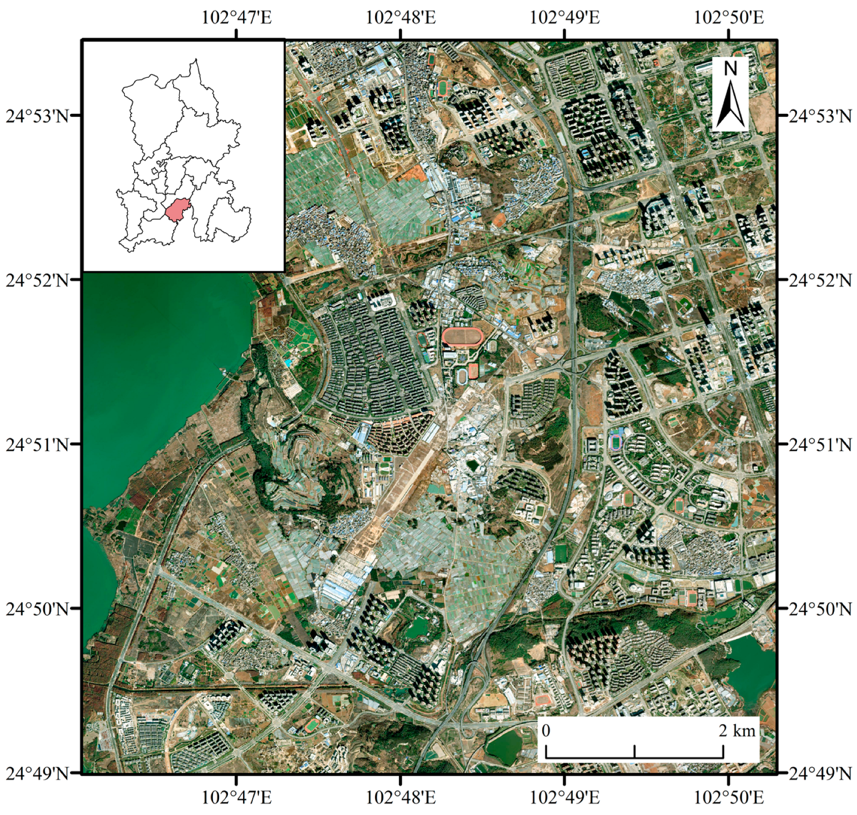
2.1. Study Area

Kunming, the capital of Yunnan Province, is located in the central part of the Yungui Plateau, between 102°10′ and 103°40′ E and 24°23′ and 26°22′ N. Chenggong District, as the administrative center of Kunming and the new campus site for several universities in Yunnan, has experienced significant urbanization in recent years (Figure 1). Dramatic changes in land use and evident population agglomeration have made it a core area characterized by dense foot traffic and frequent activity. The rapid urbanization in Chenggong District has resulted in a more complex distribution of thermal environment characteristics, making it a representative area for studying the micro-scale urban thermal environment.

2.2. Data Collection

2.2.1. Weather Station Data

This study is based on mobile observation data and recordings from the self-installed Davis weather station, aiming to analyze the thermal environment changes in Kunming’s micro-scale areas. For the mobile observation dates of 15 January 2020, and 8 January 2023, the maximum, minimum, and average temperatures were recorded to compare the weather background and thermal environment differences between the two observations. These data were obtained from the China Meteorological Data Service Center (https://data.cma.cn/) and China Weather (https://www.weather.com.cn/), providing accurate meteorological data support for the study. By comparing the temperature changes under different weather backgrounds, this study further reveals the thermal environment response differences in various urban functional areas of Kunming under different climatic conditions, offering valuable references for future urban thermal environment management and planning.

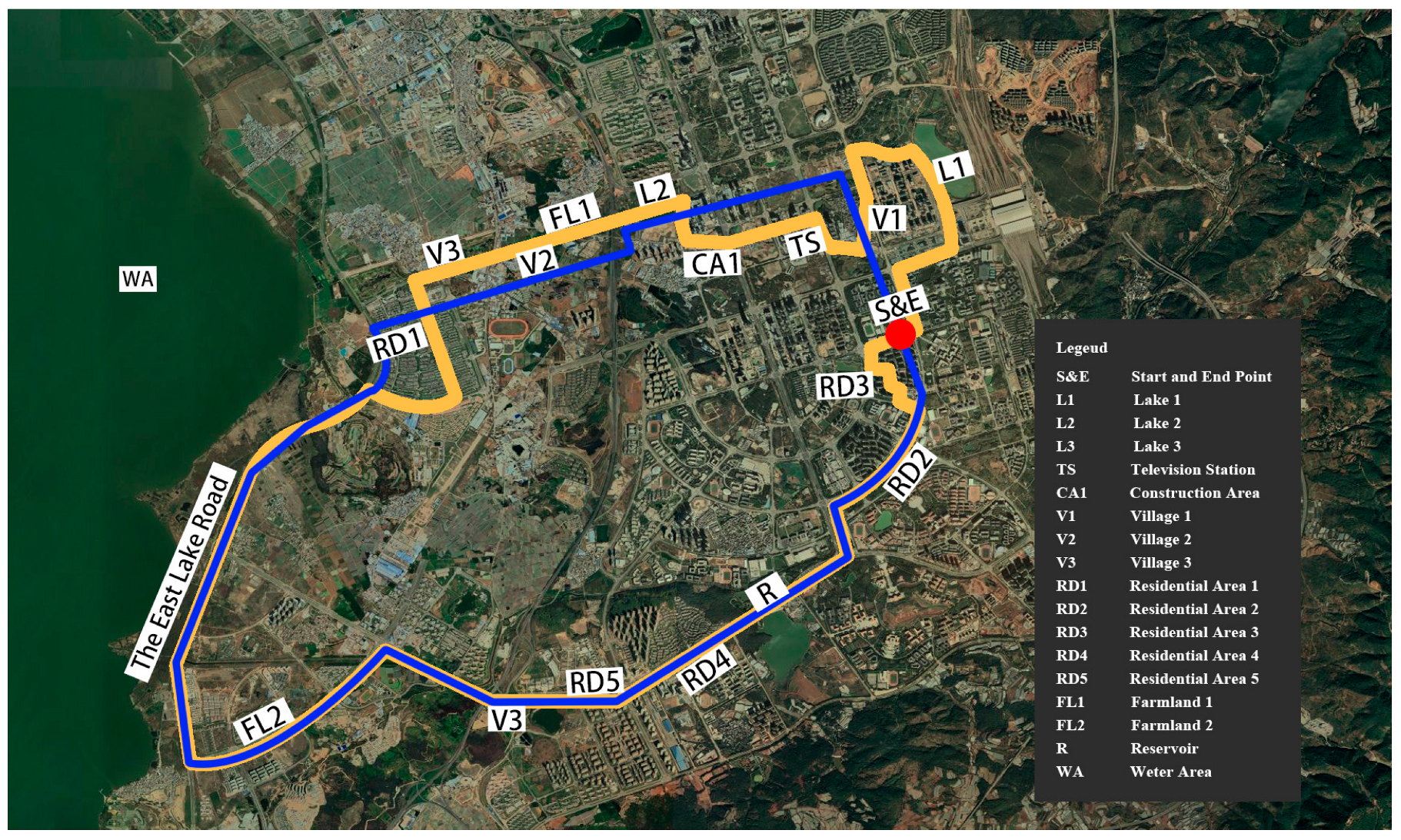
2.2.2. Mobile Observation Data

The mobile observations for this study were collected from selected areas in Chenggong District, Kunming, and temperature data were collected on 15 January 2020 and 8 January 2023, along the observation routes. These data were obtained using temperature and humidity data loggers that recorded continuously at a high density of once per second. This ensures a true representation of how temperature varies with the environment. The region includes a variety of land use types.
In selecting the mobile observation route, the primary consideration was to ensure the inclusion of a variety of typical urban functional areas. These include highly commercialized zones (such as the Rainbow Yunnan First City), residential areas (like Yuhua Yuxiu and Yimingyuan), large water bodies (such as Dianchi Lake and Pan Chun Lake), agricultural land and villages (such as Wujia Ying Village and Sanchakou Village), as well as university campuses. These areas represent different levels of human activity, land use types, and ecological characteristics, facilitating a comprehensive study of the relationship between urban heat island effects and factors like land use, greenery, and traffic flow, providing multidimensional data on thermal environment changes. The mobile observation started and ended at a highway intersection approximately 600 m northwest of Kunming South Railway Station (referred to as the Start Point and End Point, abbreviated as S&E). The total length of the route is approximately 30 km. It extends westward to Huanhu East Road near Dianchi Lake, eastward to the West Square of Kunming South Railway Station, with the northern boundary being Pan Chun Lake, also known as “Qibu Chang Datangzi.” The southernmost part of the route is along the ancient Dian Road-Yupu Road. As shown in Figure 2, the mobile testing passes through five residential districts: Dianchi Xingchen (RD1), Shuxiang Dadi (RD2), Yuhua Yuxiu (RD3), Yimingyuan (RD4), and Shidai Junyuan (RD5). It also passes through the middle of RD3, while RD1 is highly commercialized with numerous restaurants and shops. There are five water bodies: Dianchi Lake (WA), Bailongtan (L1), Pan Chun Lake (L2), Yueya Pond (L3), and Guanshan Reservoir (R). Among them, Dianchi Lake is a large water body with a total area of 330 km2, while the others are medium to small-sized water bodies. There are three villages: Wujia Ying Township (V1), Sanchakou Village (V2), and Kele Village (V3). Additionally, two agricultural fields (FL1, FL2), construction land (CA1), and Yunnan Radio and Television Station (TS) are present in the area. Table 1 presents the equipment information table.
To ensure data accuracy and consistency, the observation vehicle maintained a steady, low speed (approximately 15–20 km/h) along a pre-defined route, minimizing the impact of motion-related disturbances on the readings. Temperature and humidity sensors were mounted at the center of the vehicle roof, well away from the engine, exhaust pipes, and air conditioning vents, to avoid interference from vehicle-generated heat. Although minor short-term fluctuations may occur in complex road sections, the spatial continuity and distinguishability of the collected thermal data were well preserved. This provides a reliable basis for analyzing macro-level thermal environment patterns across different urban functional areas.

2.3. Data Processing

This study mainly conducted on-site tests using a mobile observation method. When processing the data, the methods of simultaneous correction and spatial interpolation were used to reduce errors by considering potential issues such as time errors in the test results or uneven distribution of measurement points.

2.3.1. Data Processing of Raw Data

  • Temperature Data
The HOBO-Onset MX2302A temperature data logger used for the testing was configured with the desired start time and recording interval using the computer software. Once the designated time was reached, the data logger automatically initiated the installation process and began recording the relative temperature data according to the present requirements.
2.
GPS Data
To ensure the continuity of recorded GPS trajectories, any surplus data points can be removed during the subsequent data compilation. The GPS data can then be imported into Google Earth Pro 7.1.8 to visualize the route trajectory.

2.3.2. Data Normalization

To begin the process of data normalization, the GPS trajectory data were opened, and the coordinates marking the starting and ending points identified. The raw data from both instruments were then subjected to normalization procedures. These steps involved aligning the timestamps, performing spatial interpolation, implementing simultaneous revision, and simplifying the route trajectory data.
  • Aligning Timestamps
In this study, the temperature and humidity data logger used for testing was configured to record at a frequency of one measurement per second, which aligns with the frequency of GPS recorders capturing trajectory points. This facilitates the correspondence between the data in terms of time, temperature, relative humidity, and latitude–longitude coordinates.
2.
Spatial Interpolation
During the process of mobile observation, there are often areas with significant obstructions that interfere with GPS signals, resulting in data points being lost. Therefore, it becomes necessary to utilize spatial interpolation methods to supplement the missing data points.
3.
Simultaneous Revision
During the testing period, the equation for the temperature curve trend was derived through regression analysis using hourly meteorological data recorded by the self-established Davis weather station. By applying this equation, the data was revised to a common reference time. Specifically, linear regression was selected to revise the data to the midpoint of the testing period.

2.3.3. Creating Contour Maps

To visualize the spatial distribution of temperatures across the study area, this study employed a combination of gridding and spatial interpolation techniques, which are commonly used in environmental and climatological research to reconstruct continuous surface fields from discrete observational data. In this context, longitude and latitude were used as the spatial coordinates (X and Y axes), and temperature readings served as the dependent variable (Z axis).
A geostatistical interpolation method—Ordinary Kriging—was applied using Surfer 15 software to generate a regular grid and create spatially continuous temperature fields. Kriging was chosen for its ability to incorporate spatial autocorrelation structures through semi-variogram modeling, which improves interpolation accuracy compared to deterministic methods. The experimental data underwent semi-variogram analysis, and the Gaussian model was selected for variogram fitting. Key parameters, including range, sill, and nugget, were determined empirically to reflect the spatial continuity of the temperature field. The gridding process enabled the estimation of temperature values in unsampled areas, thus capturing spatial patterns and micro-scale thermal anomalies that may not be evident from raw data alone.
A 3D wireframe model was used to represent the interpolated surface, providing an intuitive visualization of temperature fluctuations. To enhance clarity and assist in interpretation, scatter plots of measurement points were overlaid on the surface to highlight spatial correspondence between actual and interpolated values. This integrated visualization approach, grounded in geostatistics, effectively supports the identification of urban heat island dynamics and thermal environmental variations across different functional zones.

2.4. Calculating the Fluctuation in Urban Thermal Environment

The fluctuation in the urban thermal environment can be measured by calculating the temperature amplitude and standard deviation.
The temperature amplitude refers to the difference between the maximum and minimum temperatures over a specific time period. It can be calculated using Equation (1).
ΔT = TmaxTmin
where Tmax is the highest temperature during the period. Tmin is the lowest temperature during the period.
The standard deviation is a statistical measure that quantifies the dispersion of temperature data, indicating the stability of temperature fluctuations. It can be calculated using Equation (2).
σ T = 1 n i = 1 n T i T ¯ 2
where Ti is the temperature at each observation point. T ¯ is the mean temperature across all observation points. n is the number of observation points.
By calculating the temperature fluctuation amplitude and standard deviation, the temperature variability in the study area can be comprehensively assessed. The temperature fluctuation amplitude helps to directly understand the extreme temperature changes within the region, such as heat island effects or special weather phenomena, thus identifying potential anomalies. On the other hand, the standard deviation provides a more refined description of the regularity and extent of temperature fluctuations, making it suitable for in-depth analysis of the trends and stability of temperature variations. The combination of both measures allows for a more comprehensive reflection of the changes in the thermal environment of the study area.

3. Results

3.1. Distribution of the Thermal Environment

By plotting the mobile observation data, a 3D temperature distribution map of the study area is created, and this is combined with the measured temperature data to obtain the thermal environment distribution within the mobile observation area.
As shown in Figure 3, the temperature range on 15 January 2020, was from 9.0 °C to 19.4 °C, with a temperature difference of 10.4 °C. In contrast, on 8 January 2023, the temperature range expanded to 4.0 °C to 20.5 °C, with a temperature difference of 16.5 °C, indicating a significantly larger temperature variation in 2023 compared to 2020. However, according to the background temperature data on the test days shown in Table 2, the day of the first test, the maximum temperature difference was 10 °C, while on the second test day, it was 13 °C. Under the influence of background weather conditions, the study area experienced an increase in temperature differences. The temperature variation in the tested area changed from 10 °C to 10.4 °C, the temperature difference in the tested area expanded from 13 °C to 16.5 °C. From the overall temperature changes within the study area, the data collected on 8 January 2023 show more dramatic fluctuations, indicating a less stable thermal environment.

3.2. Fluctuations in the Thermal Environment

The thermal environment distribution map based on temperature data from flow observations can observe the temperature distribution in the region, but the specific fluctuation in the thermal environment requires specific statistics on the data, and in this study, the temperature difference is used for the observed data to represent the magnitude of fluctuation in the thermal environment, and the standard deviation in the temperature data is used to measure the degree of dispersion in the distribution of the temperature data.
From Table 3, it can be observed that there are significant differences in temperature variation and standard deviation between 15 January 2020, and 8 January 2023, reflecting the fluctuations in the thermal environment of the study area over the two years. During the testing period on 15 January 2020, the temperature differences were relatively small, with a maximum of 1.3 °C and a minimum of 1.0 °C. These small temperature differences indicate that, during 2020, temperature changes in the study area were relatively stable, and the thermal environment remained stable. In terms of standard deviation, the values on 15 January 2020, were relatively low, with 0.24 °C, 0.29 °C, and 0.34 °C, which further indicates that the thermal environment in 2020 had small fluctuations, with temperature changes being more regular and stable. In contrast, on 8 January 2023, the standard deviation values increased significantly, especially during the afternoon and evening periods, where the standard deviation reached 2.43 °C and 1.28 °C, respectively. These larger standard deviation values indicate that, during 2023, the temperature fluctuations in the study area were more intense, with a larger range of variation, and the thermal environment became more unstable.
In order to obtain a better view of the distribution of the mobile observations, box plots of the two sets of data were plotted, and when combined with Figure 4 and the tabular data, the temperatures in all periods of the 2023 test are lower than the 2020 results, which is consistent with the individual test days. However, the box plots provide a more visual representation of the distribution of the test data, with the shorter purple boxes indicating concentrated temperature data, less fluctuating thermal environments, and stable thermal environments, but higher overall temperatures, while the longer yellow boxes indicate more dispersed temperatures, larger regional temperature differences, and an unstable but overall cooler thermal environment. The median of the 2023 data is located at the bottom of the box while the median of the 2020 data is located at the top of the box, suggesting that the 2023 temperature data is on the cool side, with more cool readings compared to 2020, which coincides with the decrease in hotter areas seen in the 3D distribution plot.
To better compare the differences in air temperatures between different land use types, the study collected data on the average air temperatures in different urban functional areas for each time period during the two test periods (Figure 5).
Based on the test data from 15 January 2020, and 8 January 2023, a comprehensive analysis of temperature variations across different urban functional areas during various time periods reveals significant differences in thermal environment responses under different weather backgrounds. On the morning of 15 January 2020 (08:30), temperatures in industrial, residential, village, urban, and green areas were relatively high, whereas on the morning of 8 January 2023 (09:30) temperatures dropped dramatically, with the industrial area showing the most pronounced decrease of 10.2 °C, indicating an overall colder temperature background in 2023. During the afternoon test (15:30), temperatures in 2023 were generally higher than those in 2020; specifically, temperatures in the industrial, residential, and green areas increased by 15.0 °C, 7.8 °C, and 9.2 °C, respectively, while the village area increased by only about 8.5 °C, reflecting that weather conditions lead to more pronounced heat accumulation in densely built, sparsely green areas. In the evening test (20:30), temperatures in 2023 again fell below those in 2020, cooling to 11.2 °C and 5.2 °C in the industrial and residential areas, respectively, whereas the green area experienced a smaller decrease of 7.7 °C. Overall, the results indicate that temperature fluctuations in the early morning and evening of 2023 increased significantly, with industrial and residential areas being particularly sensitive to temperature changes, while green areas exhibited relatively stable temperature variations, underscoring the moderating role of the natural environment in urban thermal regulation. This analysis provides quantitative support for a better understanding of the differences in thermal feedback among various urban functional areas under different weather conditions and reveals the influence of green space and building density on temperature fluctuations in urban thermal management, offering important insights for mitigating the urban heat island effect and enhancing thermal comfort.

4. Discussion

4.1. Distribution of Thermal Environment at Different Times in the Study Area

This study compared two sets of mobile observation data from Kunming’s Chenggong District, revealing distinct thermal patterns across different urban functional areas during temperature rise, peak, and decline phases. These variations are driven mainly by surface heat capacity, urban structural features, and microclimatic factors, demonstrating the complex mechanisms governing urban thermal dynamics.
During the warming phase, the rate of temperature increase in 2023 was notably lower than in 2020. This difference can be explained by thermal inertia and radiation budget mechanisms. Vegetated areas possess lower heat capacity and thermal inertia, rapidly losing heat at night, which delays warming in the early morning hours. In contrast, densely built residential areas composed of materials with high heat capacity and thermal inertia—such as concrete and asphalt—retain residual heat from the previous day, facilitating quicker warming in the morning [28]. Furthermore, nocturnal temperature inversion in green spaces and wetlands contributes to cold air drainage effects at sunrise, further suppressing early temperature recovery [29].
At peak temperatures, both observation days reached similarly high maximum temperatures, yet spatial temperature differences expanded significantly in 2023. High-temperature zones emerged predominantly in densely constructed areas with large sky-view factors, such as university campuses and major residential complexes. In these areas, impervious surfaces dominate, reducing evapotranspiration and leading solar energy absorption primarily to sensible heat flux, thus accelerating surface heating [30]. Conversely, green spaces and water bodies mitigate heating through evapotranspiration and latent heat transfer, acting as thermal buffers. This aligns with existing urban heat island theories emphasizing the critical roles of vegetation and water bodies in maintaining localized energy balance [31].
During the cooling phase, anomalous temperature distributions observed in 2023 reveal more complex microclimate interactions. Some wetland areas exhibited higher temperatures than adjacent residential zones, highlighting the role of water bodies and high humidity in delaying heat dissipation due to greater thermal storage capacity [32]. Although built-up areas generally have higher thermal inertia, their greater sky-view factors and open spatial layouts promote efficient nocturnal radiative cooling. Additionally, nighttime urban ventilation significantly affects local thermal patterns, with areas featuring better ventilation conditions cooling more rapidly [33].
The findings derived from box plots and 3D temperature maps further confirm increased thermal variability in the 2023 dataset. Integrating these mechanism-based explanations, the study argues that the differential thermal responses across urban functional zones are governed not only by building density and vegetation coverage but also by localized radiation budgets, thermal inertia effects, and microclimatic factors. Such comprehensive understanding provides crucial insights for future climate-adaptive urban planning strategies, including optimized spatial arrangements, enhanced urban greenery, and improved thermal properties of urban construction materials to effectively manage urban thermal instability under extreme weather conditions.

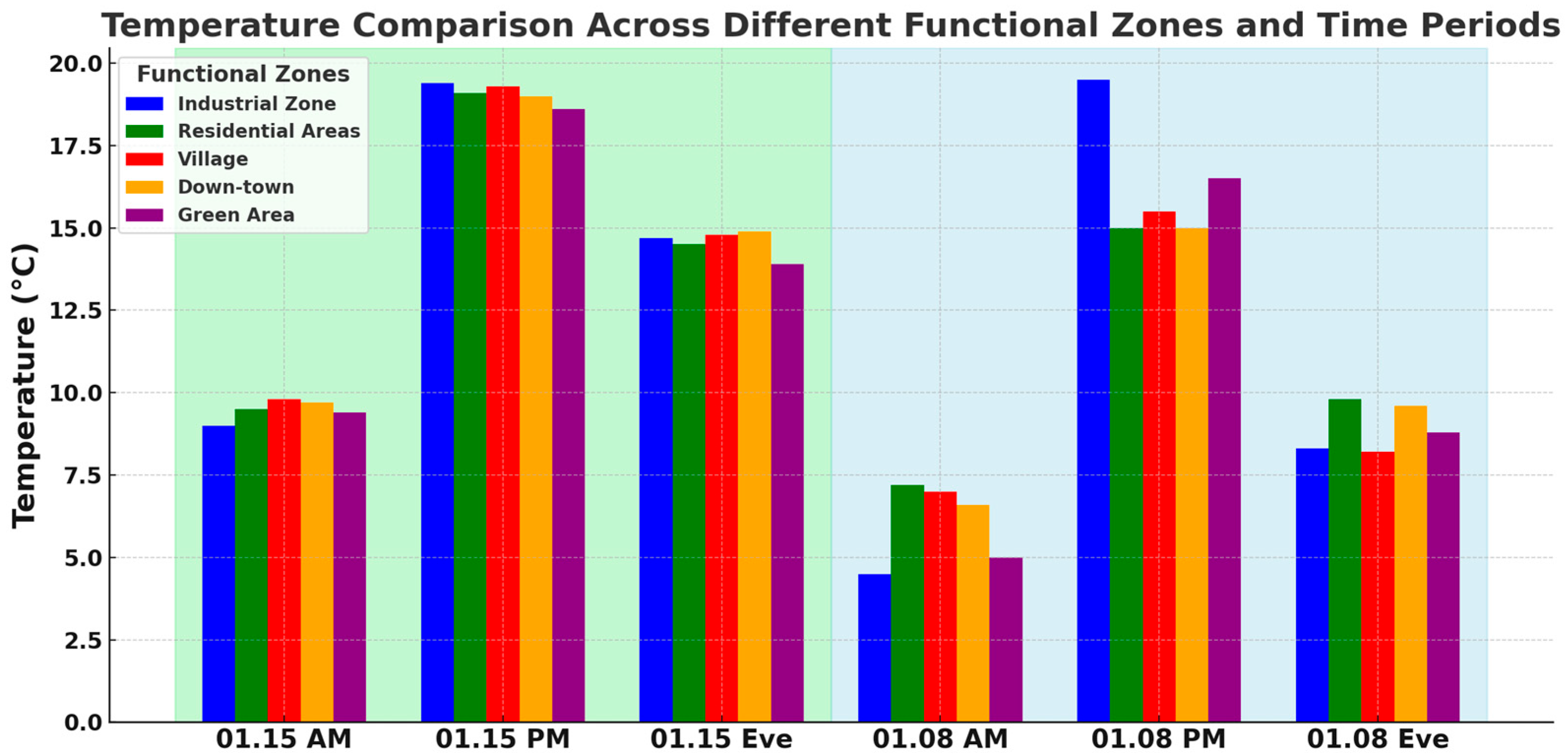
4.2. Impact of Different Urban Functional Areas on the Thermal Environment

Urban functional areas exhibit markedly different thermal responses, driven by a combination of surface cover types, building density, vegetation levels, and anthropogenic activity. In densely built zones such as industrial, commercial, and residential districts, the dominance of impervious surfaces with high heat capacity leads to significant daytime heat accumulation. However, these areas lack effective thermal buffering mechanisms, resulting in rapid nighttime heat loss and pronounced temperature fluctuations. The concentration of anthropogenic heat sources further amplifies local heat buildup and intensifies the urban heat island effect.
In contrast, natural and semi-natural areas—such as green spaces, wetlands, and villages—typically have abundant vegetation and water bodies, enabling stronger thermal regulation. Through evapotranspiration and latent heat exchange, these areas delay daytime heating and slow nighttime cooling, acting as “temperature stabilizers” under extreme weather conditions. Particularly in colder backgrounds, built-up zones with limited green infrastructure and low residual heat are more prone to overcooling, whereas vegetated areas maintain more stable thermal conditions and demonstrate greater climate resilience.
These differentiated thermal responses reflect not only the direct influence of urban land use on energy distribution but also offer theoretical guidance for thermal environment management. Future urban planning should account for the spatial coordination of functional areas, optimize building layout and density, and increase the proportion of green and blue infrastructure. Such strategies will enhance cities’ adaptive capacity to diverse climatic conditions and promote the development of resilient, livable urban environments.

4.3. Research Limitations and Future Directions

This study is limited by its short observation period, relatively narrow spatial scope, and the limited range of influencing factors considered. While mobile observation provides valuable fine-scale data, the results are based on two typical days and may not fully reflect broader seasonal or long-term patterns. Future studies could enhance the representativeness and depth of findings by extending the observation period, expanding the study area to include more diverse urban settings, and incorporating additional environmental variables such as wind, human activity, and surface characteristics. These improvements would contribute to a more comprehensive understanding of urban thermal dynamics and support more effective climate-adaptive urban planning.

5. Conclusions

This study analyzed thermal environment differences in Kunming’s Chenggong District using mobile observation data from 2020 and 2023 under contrasting weather conditions. The results show that industrial and commercial areas experienced greater temperature fluctuations, while green areas and water bodies maintained higher stability. These findings support the effectiveness of mobile sensing in capturing fine-scale urban thermal patterns and highlight the vulnerability of built-up zones to extreme weather. Three main conclusions were drawn as follows:
  • As the temperature declines, the urban thermal environment undergoes significant changes, leading to a reduction in the area of the urban heat islands and an increase in urban cold islands.
  • In response to the temperature drop, different urban functional areas exhibit varying thermal feedback, with industrial and residential areas being more sensitive to temperature changes, resulting in a distribution characterized by lower temperatures.
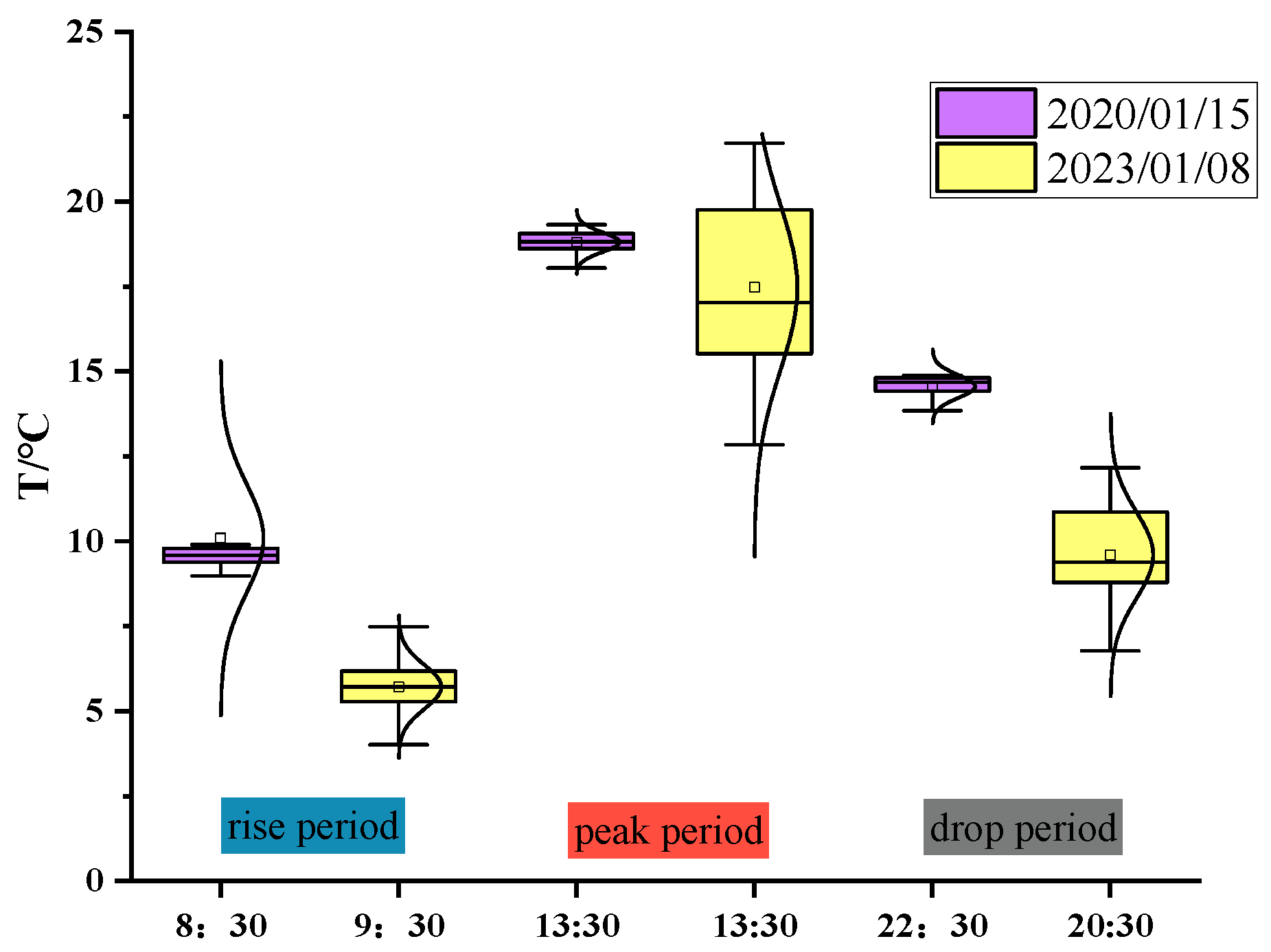
  • Temperature fluctuations in the study area have intensified; the maximum standard deviation of the 2020 test data did not exceed 0.35 °C with a temperature difference of less than 1.5 °C, whereas the standard deviation of the 2023 data increased significantly across all three periods, reaching up to 2.43 °C, and the temperature difference expanded to 7.5 °C. This indicates that the thermal environment fluctuations in the study area are significant.
These findings offer valuable implications for urban planning. In particular, the enhanced thermal stability observed in green and water-rich areas highlights the importance of increasing green space coverage and optimizing its spatial layout. Urban planners should prioritize the integration of vegetation and water bodies in densely built zones to mitigate thermal instability and improve climate resilience.

Author Contributions

Conceptualization, Z.W.; Software, Z.M.; Writing—original draft, P.Z.; Supervision, C.O. All authors have read and agreed to the published version of the manuscript.

Funding

This work was supported by the Scientific Research Foundation of Yunnan Provincial Department of Education (2024Y130).

Data Availability Statement

The original contributions presented in the study are included in the article, further inquiries can be directed to the corresponding author.

Conflicts of Interest

The authors declare no conflicts of interest.

References

  1. Oke, T.R. The energetic basis of the urban heat island. Q. J. R. Meteorol. Soc. 1982, 108, 1–24. [Google Scholar] [CrossRef]
  2. Broitman, D.; Koomen, E. Residential density change: Densification and urban expansion. Comput. Environ. Urban Syst. 2015, 54, 32–46. [Google Scholar] [CrossRef]
  3. Gao, Y.; Zhang, N.; Chen, Y.; Luo, L.; Ao, X.; Li, W. Urban heat island characteristics of Yangtze river delta in a heatwave month of 2017. Meteorol. Atmos. Phys. 2024, 136, 30. [Google Scholar] [CrossRef]
  4. Anjileli, H.; Huning, L.S.; Moftakhari, H.; Ashraf, S.; Asanjan, A.A.; Norouzi, H.; AghaKouchak, A. Extreme heat events heighten soil respiration. Sci. Rep. 2021, 11, 6632. [Google Scholar] [CrossRef] [PubMed]
  5. Oleson, K. Contrasts between Urban and Rural Climate in CCSM4 CMIP5 Climate Change Scenarios. J. Clim. 2012, 25, 1390–1412. [Google Scholar] [CrossRef]
  6. Brusseleers, L.; Nguyen, V.G.; Vu, K.C.; Dung, H.H.; Somers, B.; Verbist, B. Assessment of the impact of local climate zones on fine dust concentrations: A case study from Hanoi. Vietnam Build. Environ. 2023, 242, 110430. [Google Scholar] [CrossRef]
  7. Xi, Y.; Wang, S.; Zou, Y.; Zhou, X.; Zhang, Y. Seasonal surface urban heat island analysis based on local climate zones. Ecol. Indic. 2024, 159, 111669. [Google Scholar] [CrossRef]
  8. Ornam, K.; Wonorahardjo, S.; Triyadi, S. Several façade types for mitigating urban heat island intensity. Build. Environ. 2024, 248, 111031. [Google Scholar] [CrossRef]
  9. Zhao, J.; Zhao, X.; Liang, S.; Zhou, T.; Du, X.; Xu, P.; Wu, D. Assessing the thermal contributions of urban land cover types. Landsc. Urban. Plan. 2020, 204, 103927. [Google Scholar] [CrossRef]
  10. Shen, P.; Wang, M.; Liu, J.; Ji, Y. Hourly air temperature projection in future urban area by coupling climate change and urban heat island effect. Energy Build. 2023, 279, 112676. [Google Scholar] [CrossRef]
  11. Lin, Z.; Xu, H.; Yao, X.; Yang, C.; Ye, D. How does urban thermal environmental factors impact diurnal cycle of land surface temperature? A multi-dimensional and multi-granularity perspective. Sustain. Cities Soc. 2024, 101, 105190. [Google Scholar] [CrossRef]
  12. Stewart, I.D.; Oke, T. Local Climate Zones for Urban Temperature Studies. Bull. Am. Meteorol. Soc. 2012, 93, 1879–1900. [Google Scholar] [CrossRef]
  13. Tao, H.; Xing, J.; Pan, G.; Pleim, J.; Ran, L.; Wang, S.; Chang, X.; Li, G.; Chen, F.; Li, J. Impact of anthropogenic heat emissions on meteorological parameters and air quality in Beijing using a high-resolution model simulation. Front. Environ. Sci. Eng. 2022, 16, 44. [Google Scholar] [CrossRef]
  14. Núñez, A.; García, A.M.; Moreno, D.A.; Guantes, R. Seasonal changes dominate long-term variability of the urban air microbiome across space and time. Environ. Int. 2021, 150, 106423. [Google Scholar] [CrossRef]
  15. Klompmaker, J.O.; Hart, J.E.; James, P.; Sabath, M.B.; Wu, X.; Zanobetti, A.; Dominici, F.; Laden, F. Air pollution and cardiovascular disease hospitalization—Are associations modified by greenness, temperature and humidity? Environ. Int. 2021, 156, 106715. [Google Scholar] [CrossRef]
  16. Wu, R.; Guo, Q.; Fan, J.; Guo, C.; Wang, G.; Wu, W.; Xu, J. Association between air pollution and outpatient visits for allergic rhinitis: Effect modification by ambient temperature and relative humidity. Sci. Total Environ. 2022, 821, 152960. [Google Scholar] [CrossRef]
  17. Fang, W.; Li, Z.; Gao, J.; Meng, R.; He, G.; Hou, Z.; Zhu, S.; Zhou, M.; Zhou, C.; Xiao, Y.; et al. The joint and interaction effect of high temperature and humidity on mortality in China. Environ. Int. 2023, 171, 107669. [Google Scholar] [CrossRef]
  18. Shu, C.; Gaur, A.; Wang, L.; Lacasse, M.A. Evolution of the local climate in Montreal and Ottawa before, during and after a heatwave and the effects on urban heat islands. Sci. Total Environ. 2023, 890, 164497. [Google Scholar] [CrossRef]
  19. Zhu, Z.; Shen, Y.; Fu, W.; Zheng, D.; Huang, P.; Li, J.; Lan, Y.; Chen, Z.; Liu, Q.; Xu, X.; et al. How does 2D and 3D of urban morphology affect the seasonal land surface temperature in Island City? A block-scale perspective. Ecol. Indic. 2023, 150, 110221. [Google Scholar] [CrossRef] [PubMed]
  20. Zhou, L.; Yuan, B.; Hu, F.; Wei, C.; Dang, X.; Sun, D. Understanding the effects of 2D/3D urban morphology on land surface temperature based on local climate zones. Build. Environ. 2022, 208, 108578. [Google Scholar] [CrossRef]
  21. Das, M.; Das, A. Assessing the relationship between local climatic zones (LCZs) and land surface temperature (LST)—A case study of Sriniketan-Santiniketan Planning Area (SSPA), West Bengal, India. Urban Clim. 2020, 32, 100591. [Google Scholar] [CrossRef]
  22. Han, Y.; Qiao, D.; Zhang, Y.; Wang, J. Urban expansion dynamic and its potential effects on dry-wet circumstances in China’s national-level agricultural districts. Sci. Total Environ. 2022, 853, 158386. [Google Scholar] [CrossRef]
  23. Yuan, B.; Zhou, L.; Hu, F.; Zhang, Q. Diurnal dynamics of heat exposure in Xi’an: A perspective from local climate zone. Build. Environ. 2022, 222, 109400. [Google Scholar] [CrossRef]
  24. Wang, R.; Voogt, J.; Ren, C.; Ng, E. Spatial-temporal variations of surface urban heat island: An application of local climate zone into large Chinese cities. Build. Environ. 2022, 222, 109378. [Google Scholar] [CrossRef]
  25. Acosta, M.P.; Vahdatikhaki, F.; Santos, J.; Jarro, S.P.; Dorée, A.G. Data-driven analysis of Urban Heat Island phenomenon based on street typology. Sustain. Cities Soc. 2024, 101, 105170. [Google Scholar] [CrossRef]
  26. Kawakubo, S.; Arata, S.; Demizu, Y.; Kamata, T.; Narumi, D.; Asawa, T.; Ihara, T. Visualization of urban roadway surface temperature by applying deep learning to infrared images from mobile measurements. Sustain. Cities Soc. 2023, 99, 104991. [Google Scholar] [CrossRef]
  27. Li, X.S.; Chen, H.; Han, M.T.; Cao, J.Y. Research on the Temperature Gradients Change from Wuhan Urban Center to Suburb in Summer. Appl. Mech. Mater. 2012, 174–177, 3598–3602. [Google Scholar] [CrossRef]
  28. Kim, S.W.; Brown, R.D. Development of a micro-scale heat island (MHI) model to assess the thermal environment in urban street canyons. Renew. Sustain. Energy Rev. 2023, 184, 113598. [Google Scholar] [CrossRef]
  29. Zhang, Y.; Du, X.; Shi, Y. Effects of street canyon design on pedestrian thermal comfort in the hot-humid area of China. Int J Biometeorol. 2017, 61, 1421–1432. [Google Scholar] [CrossRef]
  30. Chang, Y.; Xiao, J.; Li, X.; Weng, Q. Monitoring diurnal dynamics of surface urban heat island for urban agglomerations using ECOSTRESS land surface temperature observations. Sustain. Cities Soc. 2023, 98, 104833. [Google Scholar] [CrossRef]
  31. Hao, L.; Huang, X.; Qin, M.; Liu, Y.; Li, W.; Sun, G. Ecohydrological Processes Explain Urban Dry Island Effects in a Wet Region, Southern China. Water Resour. Res. 2018, 54, 6757–6771. [Google Scholar] [CrossRef]
  32. Gunawardena, K.R.; Wells, M.J.; Kershaw, T. Utilising green and bluespace to mitigate urban heat island intensity. Sci. Total Environ. 2017, 584–585, 1040–1055. [Google Scholar] [CrossRef]
  33. Geng, S.; Yang, L.; Sun, Z.; Wang, Z.; Qian, J.; Jiang, C.; Wen, M. Spatiotemporal patterns and driving forces of remotely sensed urban agglomeration heat islands in South China. Sci. Total Environ. 2021, 800, 149499. [Google Scholar] [CrossRef]
Figure 1. Study area map.
Buildings 15 02517 g001
Figure 2. Mobile measurement routes. The yellow line represents the route of the first test and the blue line represents the route of the second test. The red dots indicate the start and end points of the test.
Buildings 15 02517 g002
Figure 3. Mobile observation 3D temperature distribution map: (a,c,e) represent the data from 15 January 2020, while (b,d,f) represent the data from 8 January 2023. Red pentagrams represent the hottest regions, while yellow triangles indicate the coldest regions.
Buildings 15 02517 g003
Figure 4. Box plot of regional temperatures: purple for 2020 test data, yellow for 2023. Blue area compares temperatures during warming periods, red and gray for peak and falling periods, respectively.
Buildings 15 02517 g004
Figure 5. Temperature comparison of different urban functional areas, with green and blue backgrounds representing the test data on 15 January 2020, and 8 January 2023, respectively.
Buildings 15 02517 g005
Table 1. Specifications of mobile observation instruments used for urban thermal environment monitoring.
EquipmentModesLegendsSpecifications
Professional GPS Data Logger/United States of America/Onset Computer Corporation CompanyColumbus
P-1
Buildings 15 02517 i001The positioning accuracy of the GPS is 1.5 m (horizontal) at 50% CEP (circular error probable) and 4.0 m at 95% CEP.
Temperature/RH Data Logger/Canada/Canada GPS CompanyOnset
MX2302A
Buildings 15 02517 i002This device has a temperature range of −40 °C to 70 °C, with measurement accuracies of ±0.25 °C below freezing and ±0.2 °C above, and a fine resolution of 0.04 °C.
Vehicle-mounted mobile measurement device
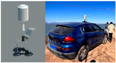
Buildings 15 02517 i003/
Table 2. Temperatures on testing dates.
Test DateTmin/°CTmax/°CΔT/°CMATmax/°CMATmin/°C
15 January 2020
8 January 2023
9
3
19
16
10
13
19
16
10
13
Note: MAT (monthly average temperature).
Table 3. Thermal environment fluctuation data within the area.
Test DateTesting TimeTmax/°CTmin/°CΔT/°CσT/°C
15 January 202008:30
15:30
20:30
9.9
19.3
14.9
8.9
18.0
13.7
1.0
1.3
1.2
0.24
0.29
0.34
8 January 202309:30
15:30
20:30
7.8
20.5
12.4
4.0
13.0
8.0
3.8
7.5
4.4
0.60
2.43
1.28
Disclaimer/Publisher’s Note: The statements, opinions and data contained in all publications are solely those of the individual author(s) and contributor(s) and not of MDPI and/or the editor(s). MDPI and/or the editor(s) disclaim responsibility for any injury to people or property resulting from any ideas, methods, instructions or products referred to in the content.

