Numerical and Experimental Analysis of Thermal Stratification in Locally Heated Residential Spaces

Abstract

This study investigates the limitations of localized heating in a single-story dwelling, using a validated computational fluid dynamics (CFD) model to analyze thermal stratification and its impact on occupant comfort. A comparative evaluation of turbulence models (k-ε and k-ω SST) and equations of state (Soave–Redlich–Kwong and Peng–Robinson) identified the k-ω SST model with the Soave–Redlich–Kwong equation as the most accurate and computationally efficient combination for capturing temperature gradients and achieving rapid convergence. Experimental validation demonstrated strong agreement between simulated and measured temperature profiles, confirming the model’s reliability. The results highlight a fundamental trade-off between localized thermal comfort and overall indoor temperature uniformity in conventionally heated spaces. While localized heating enhances comfort near the heat source, it generates vertical temperature disparities exceeding acceptable comfort thresholds at greater distances. Specifically, at 3 m from the heat source, the temperature difference between ankle and head height reached 6 °C, surpassing the 4 °C limit recommended by ASHRAE-55 for standing occupants. These findings underscore the need for alternative heating solutions that prioritize uniform heat distribution, energy efficiency, and optimized ventilation to improve indoor thermal comfort in residential buildings. This study provides critical insights to help develop and implement sustainable heating strategies and the design of energy-efficient dwellings.

1. Introduction

Addressing global environmental challenges and improving the quality of life worldwide are major focuses of current multidisciplinary research and development efforts. Several studies have examined environmental challenges [1], occupant well-being [2], and emerging technological innovations [3], each emphasizing the importance of improving living conditions and reducing environmental impact. In particular, thermal stratification in the built environment can significantly influence both indoor comfort and energy consumption. For instance, Mba et al. [4] explored floor-level ventilation strategies in hot–humid climates, while Lee et al. [5] evaluated phase-change materials for enhancing indoor temperature distribution through night ventilation. Further work by Longhitano et al. [6] investigated different air conditioning systems for addressing stratification challenges in conference rooms, whereas Wu et al. [7] demonstrated how ceiling-cooling methods can improve indoor air distribution. Providing comfortable indoor environments is crucial, as people spend approximately 90% of their time in indoor spaces, primarily at home or work [8]. Thermal comfort is a key characteristic of these spaces and can be defined as the condition that provides satisfaction with the thermal environment [9]. However, this definition is inherently ambiguous, as thermal comfort is a complex interplay of physical, physiological, and psychological factors [10,11].

Thermal stratification arises when buoyancy forces drive warm air upward and cooler air toward the floor [12], thereby producing vertical temperature gradients within the space [13]. Several authors have proposed acceptable vertical temperature gradients that extend from about 3 °C/m to as high as 8 °C/m. For instance, Liu et al. [12] found that exceeding certain gradient thresholds increases occupant dissatisfaction, while Wvon and Sandberg [14] documented growing discomfort as vertical temperature differences became more pronounced. Tanaka et al. [15] and Yu et al. [16] similarly reported adverse physiological reactions tied to larger gradients, and more recent findings by Liu et al. [17] underscore the influence of ankle-level drafts on occupant perception of comfort. Despite this variability, Olesen et al. [18] and ASHRAE-55 [19] recommend a more conservative maximum difference of 3 °C for seated occupants and 4 °C for standing occupants, making these thresholds the most widely accepted standard. Beyond temperature gradients, Fanger’s predicted mean vote (PMV) concept [20,21] highlights the influence of additional factors on thermal comfort, including humidity, air velocity, clothing, and activity level [22]. Recent works have synthesized research on thermal comfort and ventilation across various building types, identifying the need for tailored approaches in different environments [23]. Furthermore, research has shown that socioeconomic factors can also impact thermal comfort perceptions, particularly among specific demographics like Chilean school-aged children [24]. The PMV index reflects the average perception of a group but does not guarantee individual comfort. The ISO 7730 standard [25] addresses this limitation by introducing the Predicted Percentage Dissatisfaction index, which estimates the proportion of dissatisfied occupants [26].

Recent studies have highlighted the critical role of localized heating devices in enhancing thermal comfort within various indoor spaces. Yang et al. [27] examined the effects of such devices in low-temperature environments, demonstrating a marked improvement in occupant comfort and satisfaction levels, while Lee et al. [28] evaluated heated window systems for energy demand reduction and the optimization of indoor thermal conditions through simulations. Moreover, Hu et al. [29] investigated personal comfort to demonstrate that integrated heating methods can significantly enhance thermal environments. Additionally, Sauerwein et al. [30] combined experimental and numerical analyses to show that even unrenovated building stock can achieve substantial temperature reductions while maintaining occupant comfort, thereby enabling greater integration of renewable heat sources. The findings from these studies contribute to an evolving understanding of how localized heating solutions can effectively address thermal stratification and improve occupant comfort.

While computational fluid dynamics (CFD) has been widely employed to analyze indoor airflow [31] and thermal patterns [32], limited research has focused on combining CFD with experimental validation to address the specific challenges of localized heating. This combined approach enhances our understanding of stove-based systems by bridging accurate fluid-flow and heat-transfer predictions with occupant-centered metrics of thermal comfort. Computational models and experimental measurements in recent studies have been used to evaluate thermal comfort in indoor environments, enabling researchers to investigate occupant experiences and assess the performance of HVAC systems [33]. This technology has been instrumental in evaluating and optimizing heating strategies to enhance occupant comfort while minimizing energy consumption [34,35]. Previous research utilizing CFD has explored diverse aspects of thermal comfort, including the impact of thermal stratification on HVAC energy consumption in an atrium building [36], the performance of pulsating jet ventilation compared to wall displacement ventilation [37], and the analysis of indoor thermal environments and energy consumption in passive houses [38]. Recent advancements have seen the integration of machine learning techniques with CFD modeling to enhance the predictive accuracy of thermal comfort assessments. This integration enables real-time adjustments to environmental controls based on occupant feedback and behavior patterns, potentially leading to increased overall satisfaction with the indoor climate [34].

Despite these advances, a major gap remains in understanding how to assess and mitigate thermal stratification caused by localized heating systems, such as wood-burning stoves common in southern Chile [39]. The use of fuelwood as a primary heating source in this region has resulted in elevated levels of air pollution from residential wood burning [40]. This problem is exacerbated by poorly designed home insulation and the use of low-quality wood for heating. While current efforts to mitigate air pollution from wood stoves [41,42,43] focus on finding more efficient heating sources, a comprehensive understanding of the interplay between local heating, thermal stratification, and occupant comfort is critical to developing effective solutions.

This study addresses this gap by performing a comprehensive evaluation of thermal comfort in a single-story, stove-heated room using both CFD simulations and experimental measurements. This integrated approach takes advantage of the strengths of both methods: CFD modeling provides an in-depth determination of airflow patterns and temperature distributions, while experimental validation ensures the accuracy and reliability of the simulations. By incorporating the PMV index and ASHRAE Standard 55 criteria for acceptable vertical temperature gradients, this research provides a robust assessment of occupant comfort in a stratified indoor environment.

The novelty of this study lies in the systematic integration of CFD with established thermal comfort standards (e.g., the PMV index and ASHRAE-55 criteria) to more effectively investigate the specific challenges posed by stove-based heating systems. By coupling detailed CFD analyses of airflow and temperature fields with occupant-centered comfort metrics, we can directly connect predicted thermal stratification patterns to real-world comfort implications. This approach not only allows for a comprehensive analysis of how thermal stratification, driven by localized heating, affects vertical temperature gradients and potentially leads to discomfort, but also facilitates the identification of design or operational strategies that enhance indoor comfort. Consequently, the combined use of CFD tools and thermal comfort standards ensures that predicted flow distributions are interpreted within accepted thresholds for occupant satisfaction, ultimately helping develop and implement more uniform heating solutions in single-story homes that rely on wood stoves.

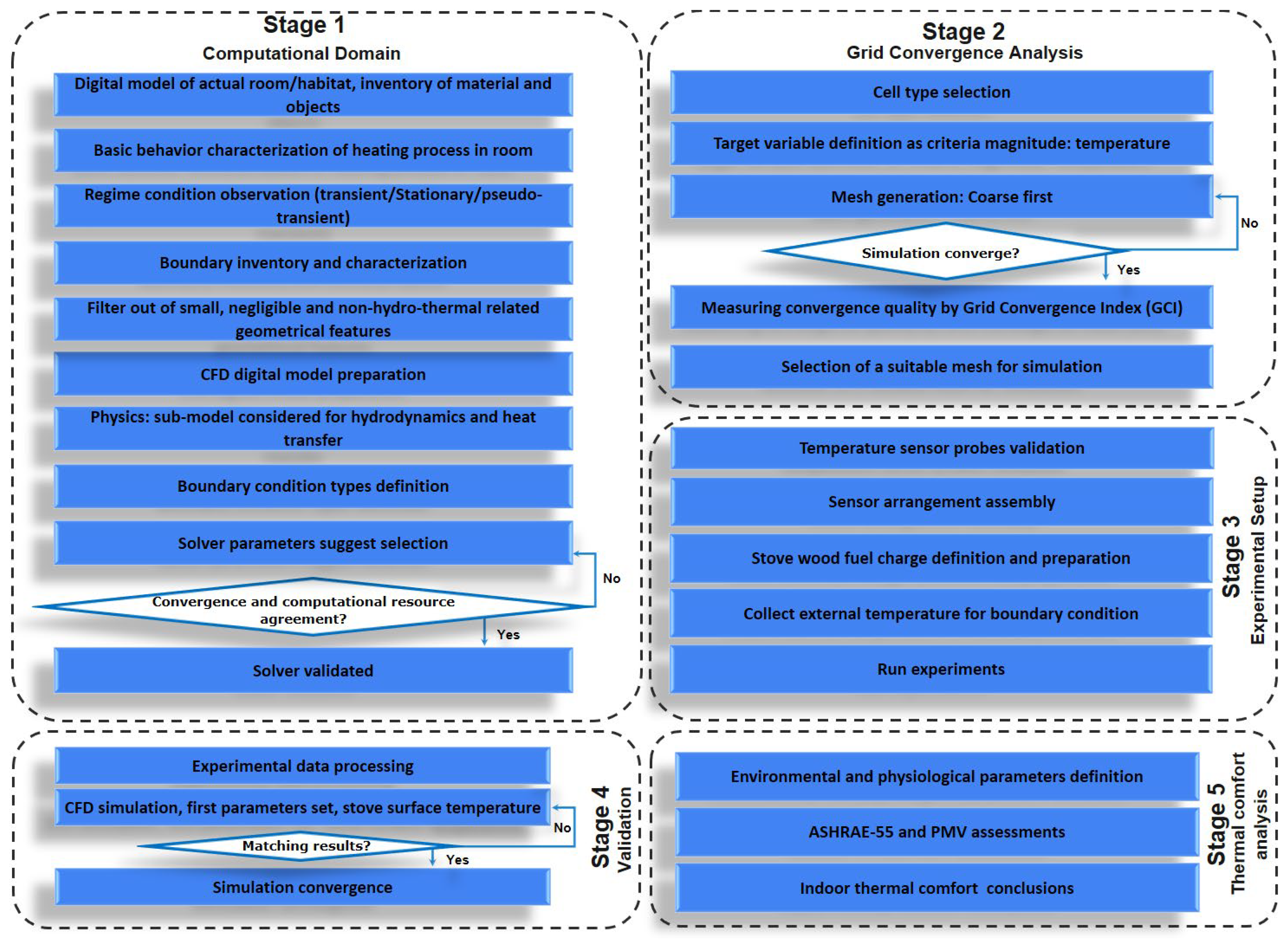
2. Materials and Methods for Capturing Thermal Stratification

This study uses computational fluid dynamics with ANSYS Fluent 2022 R21 to simulate and analyze thermal stratification within a one-story room heated by a stove. Five distinct stages are applied in this study (Figure 1).

The stages include the design of a computational domain to recreate the studied laboratory room and conditions (Stage 1), the selection of a suitable meshing (Stage 2), the experimental setup (Stage 3), model validation (Stage 4), and thermal comfort assessment (Stage 5). To ensure the accuracy of the CFD model, a rigorous two-step process adapted from Hajdukiewicz et al. [44] is employed. First, mesh independence is verified by systematically refining the mesh until the simulation results stabilize, indicating that further reductions in element size have a negligible impact (Stage 2). This ensures that the chosen mesh accurately captures the flow physics without introducing numerical errors. Second, the CFD model is validated against experimental data collected in the physical space (Stage 4). This involves comparing simulated and measured temperature profiles at various locations and time points to confirm the model’s ability to accurately represent real-world conditions.

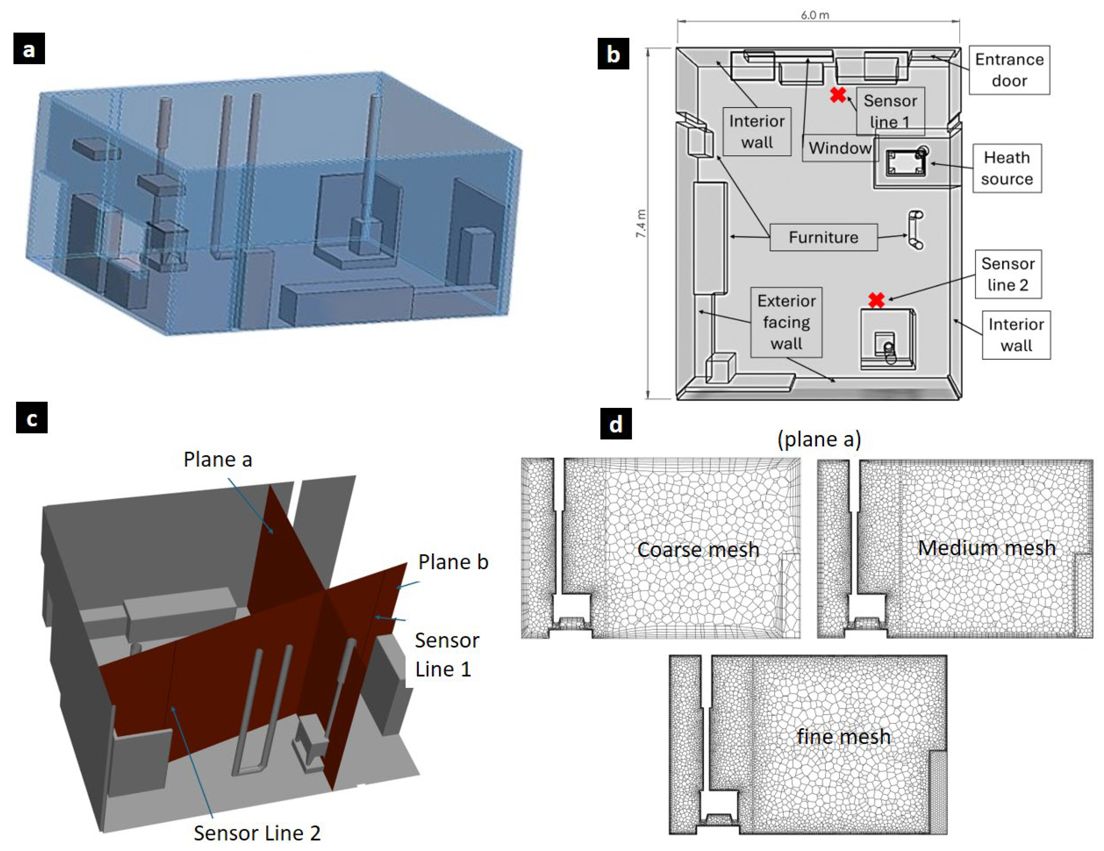
2.1. Computational Model of the Simulated Space Domain

In this study, a laboratory in the Mechanical Engineering Department of the Universidad de La Frontera is used for simulation and validation purposes. This controlled environment, shown in Figure 2a, is equipped with various pieces of furniture (chairs, desks, etc.) and wood stove emission analysis equipment, providing an ideal setting to calibrate and validate the computational model for future applications. Figure 2b shows the spatial layout of the room, including walls, furniture, and the heat source, while

Table 1. Boundary conditions.

Boundary	Material	Wall Thickness [m]	Temperature (°C)
Exterior facing wall	Concrete	0.1	10
Interior wall			15
Floor			15
Furniture	Plywood	0.02	(0 W/m2 assiged heat flux)
Ceiling	Plastic	0.02	15
Window	Glass	0.0015	10
Entrance door	Plywood	0.1	10
Heat source	Carbon steel 1020	0.002	102

details the specific boundary conditions used in the computational model. Two planes, shown in Figure 2c, are defined within the computational domain: Plane “a” is transverse to the heat source, while Plane “b” includes the locations of the temperature sensors in the physical space. Two sensor lines, labeled Line 1 and Line 2, are positioned 1.5 m and 3 m from the heat source, respectively, each consisting of eight sensors placed at heights of 0.1, 0.6, 1.2, 1.5, 1.8, 2.2, 3.0, and 3.5 m, matching the setup in the actual room.

To replicate real indoor heat losses, we assigned boundary temperatures for walls, windows, and the entrance door based on measured surface conditions (Table 1). This approach captures conduction heat losses. Our method is validated by the close match between simulated and measured temperature profiles (see Section 3.2), which differed by only ±1–2 °C at most sensor heights. This setup ensures that realistic heat-exchange processes are fully accounted for throughout the simulation.

To ensure that the simulation results are independent of the mesh size [45,46,47], three computational grids with systematically smaller cell sizes are used [48], consisting of 267,817 cells (coarse), 411,124 cells (medium), and 1,074,237 cells (fine). The grid convergence index (GCI) method, which is based on Richardson’s extrapolation [28,49], is the selected approach for determining the appropriate mesh resolution. This rigorous technique analyzes the results from the three grid resolutions to quantify the level of grid convergence and identify the mesh size that yields a solution independent of the spatial discretization. The extrapolated curve is obtained by applying Richardson extrapolation at each height presenting results of interest. To determine the characteristic mesh element size h for each mesh, Equation (1) is used

$$h={\left[{\displaystyle \frac{1}{N}}\sum _1^N{V}_{em}\right]}^{1/3}$$

(1)

where N represents the number of cells in a mesh and $V_{em}$ is the domain volume. The refinement factor between meshes is calculated using Equations (2) and (3)

$$r_{21}={\displaystyle \frac{h_2}{h_1 }}$$

(2)

$$r_{32}={\displaystyle \frac{h_3}{h_2}}$$

(3)

where $h_1<h_2<h_3$. The results for each mesh are denoted as ${\widehat{f}}_1$, ${\widehat{f}}_2$ y ${\widehat{f}}_3$. The apparent order $\left(p\right)$ is determined using Equation (4):

$$p={\displaystyle \frac{\left|ln ln\left(\left|\frac{{\widehat{f}}_3-{\widehat{f}}_2}{{\widehat{f}}_2-{\widehat{f}}_1}\right|\right)+ln ln\left(\frac{r_{21}^p-s}{r_{32}^p-s}\right)\right|}{ln ln\left(r_{21}\right)}}$$

(4)

where $s=1\cdot sgn{\displaystyle \frac{\widehat{f_3}-\widehat{f_2}}{\widehat{f_2}-{\widehat{f}}_1}}$. The GCI quantifies the relationship between mesh size change and error variation, calculated using

$$GCI={\displaystyle \frac{F\left|\epsilon \right|}{r^p-1}}$$

(5)

with relative errors

$${\epsilon }_{21}={\displaystyle \frac{{\widehat{f}}_1-{\widehat{f}}_2}{{\widehat{f}}_1}}$$

(6)

$${\epsilon }_{32}={\displaystyle \frac{{\widehat{f}}_2-{\widehat{f}}_3}{{\widehat{f}}_2}}$$

(7)

A safety factor F, typically 1.25, is included. The Richardson extrapolated result, representing the asymptotic value for a mesh with infinitesimally small cell size, is calculated using Equation (8)

$${\widehat{f}}_{ext}^{21}={\displaystyle \frac{r_{21}^p{\widehat{f}}_1-{\widehat{f}}_2}{r_{21}^p-1}}$$

(8)

This methodology ensures the accuracy and reliability of the GCI values and provides a robust framework for selecting mesh resolutions that yield spatially independent solutions. Cross-sections of these meshes along “plane a” are shown in Figure 2d. Mesh refinement was primarily focused on wall-adjacent cells, with element sizes varying from coarse to fine mesh, while elements in the domain center remained constant. The study employed polyhedral meshes, exhibiting high orthogonal quality, with 95% of elements having orthogonality values exceeding 0.98. Table 1 presents the conditions used for grid convergence index determination, along with the material properties of the simulated space, obtained from the Ansys Granta material library.

The boundary conditions described in Table 1 were applied in four steady-state simulations. These four cases result from the combination of two equations of state with two turbulence models (k-ω SST and k-ε). These equations of state were selected because they are the most successful cubic equations of state [50]. The k-ε turbulence model was chosen because it converges rapidly and accurately for different fluid regimes [51]. Finally, the k-ω SST model was used because of its excellent performance in predicting velocity and temperature in natural convection scenarios [52,53].

This study adopted a steady-state approach to approximate the quasi-equilibrium condition in the test room during prolonged stove operation. In practice, once the stove has been burning for sufficient time, temperatures and airflow patterns become relatively stable, justifying a steady-state assumption. Although strictly transient effects (such as ignition phase) are not captured, comparing simulation outputs to experimental data at multiple time points (Section 3.2) demonstrates that the steady-state CFD solution closely represents typical operating conditions in real usage.

2.2. Selection Criteria for Thermal Comfort Analysis

It is generally agreed that thermal comfort refers to the mental condition that provides satisfaction with the thermal environment [9,10]. This definition, although ambiguous, highlights the fact that comfort assessment is a cognitive process influenced by a variety of factors, including physical, physiological, and even psychological processes. In this study, in addition to the temperature gradient criteria proposed by Olesen, the Predicted Mean Vote index developed by Fanger will be used to assess thermal comfort within the space. The application of this methodology is facilitated by the use of the open-source interactive visualization tool CBE Thermal Comfort Tool developed by Tartarini et al. [54,55]. The PMV index estimates the average thermal sensation of a group of occupants exposed to the same environment, expressed on a thermal sensation scale (Equation (9)). The thermal sensation scale ranges from +3 for a hot thermal state to −3 for a cold thermal state, with intermediate values of +2 for a warm sensation, +1 for a slightly warm state, 0 for a neutral thermal sensation, −1 for a slightly cool state, and −2 for a cool thermal state [44].

$$PMV=L\left(0.303e^{-0.036M}+0.028\right)$$

(9)

The heat load of the body, represented by $L$, is defined as the difference between internal heat production and heat loss while in a comfortable situation. The metabolic rate, represented by $M$, measures the conversion of chemical energy into heat and work. $L$ can be calculated via Equation (10). Other factors that need to be considered include $Q$ (effective mechanical power), $y_T$ (air temperature), $p_a$ (water vapor pressure in the air), $t_{cl}$ (clothing surface temperature), $h_c$ (convective heat transfer coefficient), $I_{cl}$ (clothing insulation), $f_{cl}$ (clothing area factor), and $v_a$ (air velocity). Equations (11)–(14) can be used to determine the surface temperature of the clothing, the convective heat transfer coefficient, and the clothing area factor.

$$\begin{gathered} L=\left(M-Q\right)-0.0014M\left(34-y_T\mathrm{ }\right)-3.05\cdot {10}^{-3}\mathrm{ }\left(5733-6.99\left(M-Q\right)-p_a\mathrm{ }\right) \\ -0.42\left(M-Q-58.15\right)-1.72\cdot {10}^{-5}\mathrm{ }M\left(5867-p_a\mathrm{ }\right) \\ -39.6\cdot {10}^9\mathrm{ }{f}_{cl}\mathrm{ }({\left(t_{cl}+273\right)}^4-{\left(\overline{t_r}\mathrm{ }\mathrm{ }+273\right)}^4\mathrm{ })-f_{cl}\cdot \mathrm{ }{h}_c\mathrm{ }\left(t_{cl}-y_T\mathrm{ }\right) \end{gathered}$$

(10)

$$\begin{gathered} t_{cl}=35.7-0.028\left(M-Q\right) \\ -0.155I_{cl}(39.6\cdot {10}^{-9}{f}_{cl}{\left(t_{cl}+273\right)}^4-{\left(\overline{t_r}+273\right)}^4) \\ +f_{cl}\cdot h_c\left(t_{cl}-y_T\right) \end{gathered}$$

(11)

$$hc=\left\{\begin{array}{c}2.38{(t_{cl}-y_T)}^{0.25},\hspace{1em}\hspace{1em}\hspace{1em}A>12.1\sqrt{v_a}\\ 12.1\sqrt{v_a},\hspace{1em}\hspace{1em}A\le 12.1\sqrt{v_a}\end{array}\right.$$

(12)

$$A=2.38{\left(t_{cl}-y_T\right)}^{0.25}$$

(13)

$$f_{cl}=\left\{\begin{array}{c}1+0.2I_{cl},\hspace{1em}{I}_{cl}\le 0.5clo\\ 1.05+0.1I_{cl},\hspace{1em}{I}_{cl}>0.5clo\end{array}\right.$$

(14)

2.3. Experimental Data Acquisition and Postprocessing of Temporal-Specific Temperature Data

The reliability of the CFD method is verified by comparing the simulation results with the experimental data. For this purpose, two sets of DS18B20 digital thermal sensors were installed (Figure 2c). The first set was placed horizontally 1.5 m away from the heat source, and the second set was placed 3 m away, as shown in Figure 2b. Each set consists of 8 probes placed at 0.1, 0.6, 1.2, 1.5, 1.8, 2.2, 3, and 3.5 m in height.

The DS18B20 temperature sensor has been widely employed across various fields. Wang et al. [56] integrated the sensor into a high-precision system for air temperature data acquisition, which also included pressure measurements. Fathoni et al. [57] utilized the DS18B20 in their adaptation of a hot water dispenser designed for visually impaired individuals. Similarly, Xu et al. [58] chose the sensor for its rapid response, speed, low power consumption, and reliability in their design of a portable refrigerator.

For experimental data collection, a wood stove served as the heat source, complemented by the previously mentioned temperature sensor array. To ensure experimental replicability, a standardized biomass loading method was established. Noise reduction in the acquired data was achieved using a Savitzky–Golay filter, a method known for its ability to preserve significant signal features such as peaks and valleys [59]. This approach involves fitting a low-degree polynomial to a sliding window of data points, with the smoothed signal estimated from these local approximations [60]. Implementation was carried out in MATLAB 2023b [61,62], employing a polynomial order of 1 and a frame length of 201.

To ensure experimental repeatability, a standardized biomass loading protocol was implemented, involving the controlled combustion of eucalyptus wood pieces (25 × 4 × 4 cm) in quantities of 1.8 kg, 1.6 kg, and 1.4 kg per test run. The stove was placed on a precision balance to monitor real-time fuel consumption. Temperature data were recorded using DS18B20 sensors at eight heights, connected from a 1-Wire protocol to an Arduino UNO board, with data acquired at 1 s intervals and post-processing carried out using Excel-based filtering techniques.

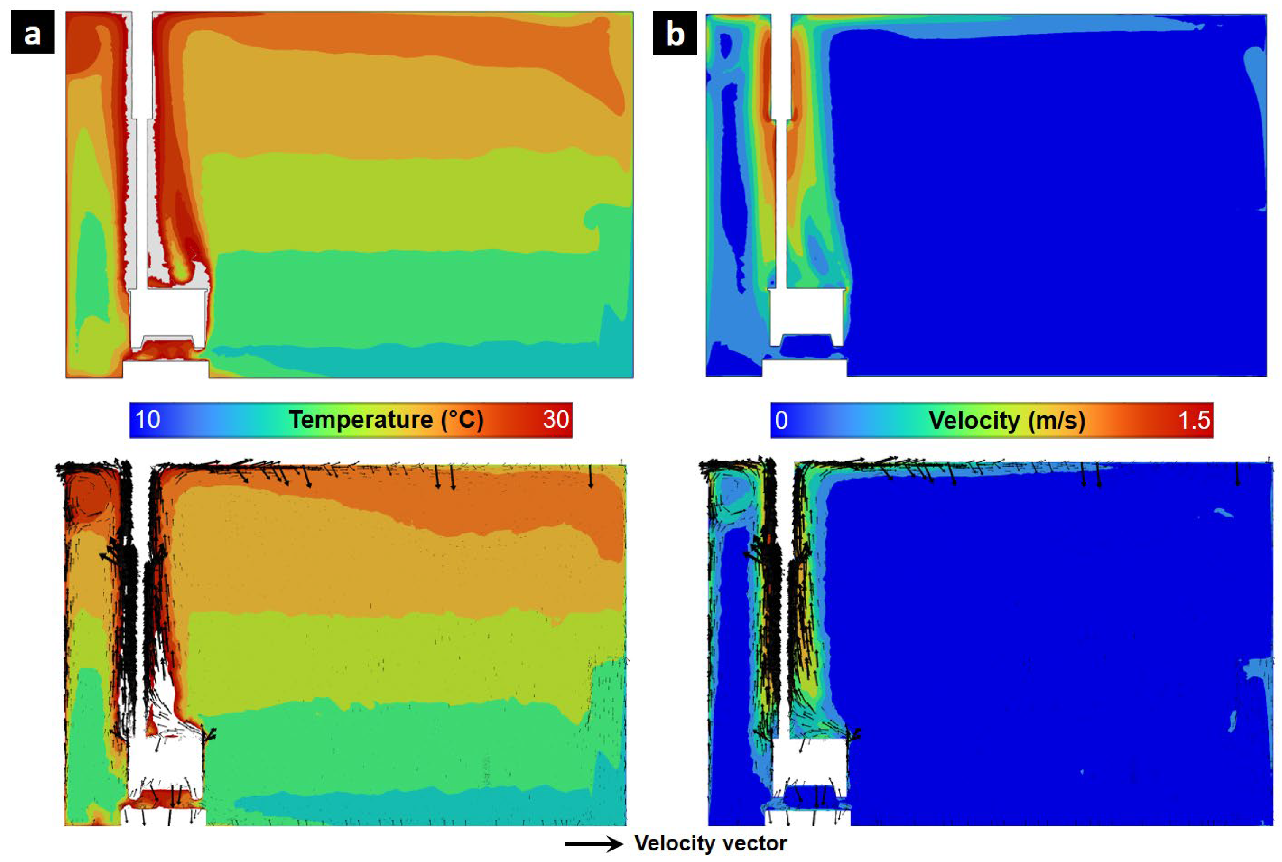
3. Results of Thermal Stratification Analysis Using CFD and Experimental Validation

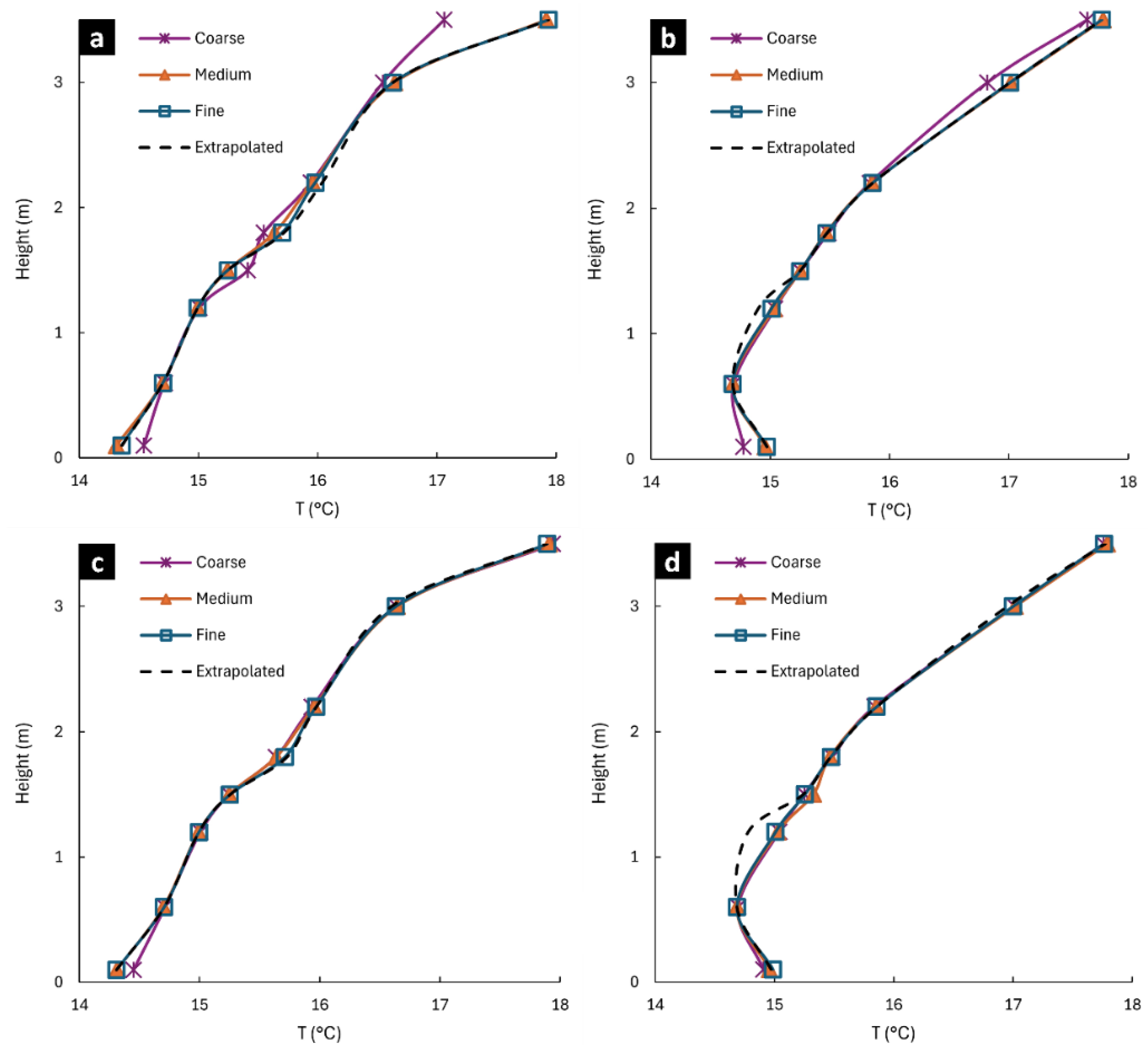
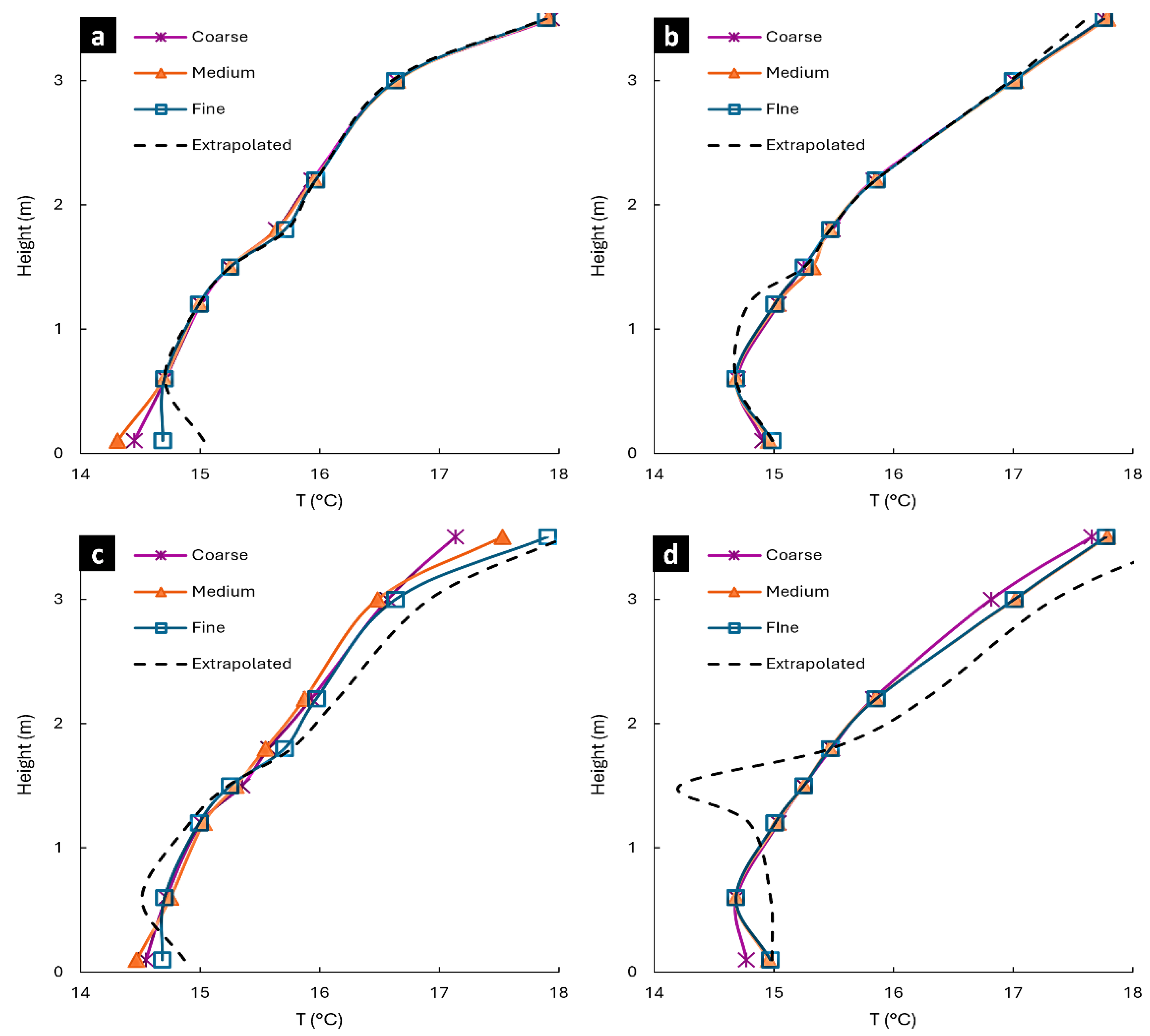
3.1. Temperature Gradient Predictions and Mesh Convergence Analysis in CFD Simulations

Figure 3 and Figure 4 show Richardson extrapolated temperature profiles for different turbulence models, equations of state, and distances from the heat source, illustrating temperature distributions and mesh resolution effects. The extrapolated curves indicate how effectively each turbulence model/equation-of-state combination captures the asymptotic solution, thereby revealing differences in their ability to resolve temperature variations across mesh refinements. The slight temperature drops observed at certain heights are due to small intermesh variations during extrapolation and reflect localized convective currents as cool air descends away from the stove. The Soave–Redlich–Kwong (SRK) equation of state paired with the k-ω SST turbulence model yielded faster convergence and more accurate agreement with extrapolated solutions. Conversely, the Peng–Robinson (PR) equation with the k-ε turbulence model combination showed slower convergence and larger discrepancies, especially near the heat source at 1.5 m. The k-ω SST model excels at capturing near-wall turbulence and buoyancy-driven flows, and SRK reliably predicts thermodynamic properties in steep gradients, leading to faster and more accurate convergence than the PR–k-ε approach. As shown in

Table 2. Average grid convergence index (GCI) for different state equations and turbulence models across medium and fine meshes.

Equation of State	Turbulence Model	Average GCI Fine Mesh (%)	Average GCI Medium Mesh (%)
SRK	k-ω SST	0.0985	0.2215
	k-ε	0.459	1.117
PR	k-ω SST	0.402	0.429
	k-ε	1.555	1.980

, this advantage is most evident under steep vertical gradients near the stove.

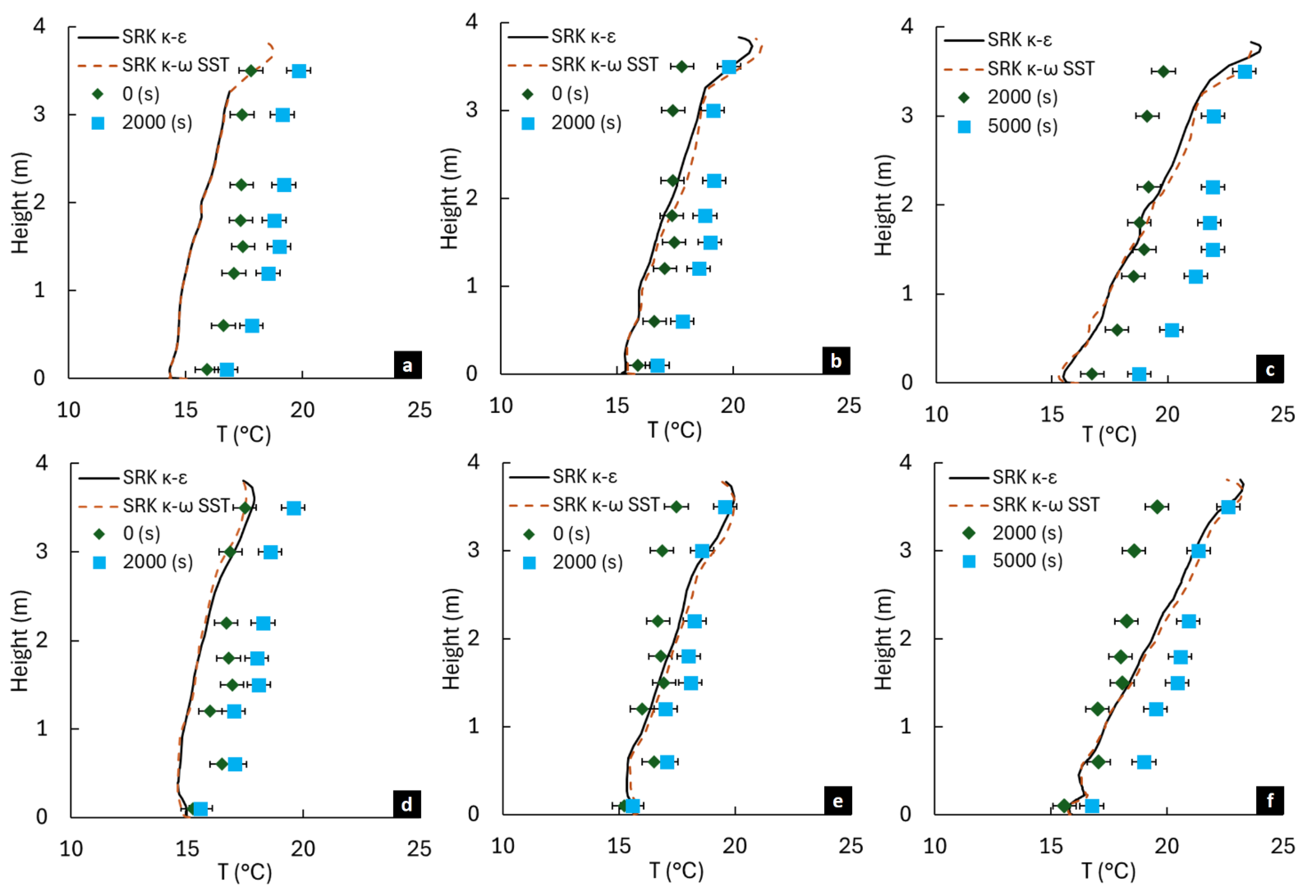
3.2. Thermal Stratification Profile: Experiments Versus Computational Modeling

Thermal stratification in indoor environments heated by localized sources is a critical factor affecting occupant comfort and energy efficiency. To evaluate the performance of the CFD model in capturing thermal stratification patterns, temperature, and velocity fields were analyzed in conjunction with experimental data. Figure 5 provides a visualization of the simulated thermal and velocity fields, while Figure 6 compares simulated temperature profiles using the k-ε and k-ω SST turbulence models against experimental measurements along two sensor lines. Both models are compared to experimental data to further validate the superiority of the k-ω SST model against the k-ε model under the specific scenarios of thermal stratification. Figure 5a shows the temperature field within the room, highlighting the vertical thermal stratification induced by localized heating. The temperature near the stove reaches approximately 30 °C and decreases with height, with values approaching 10 °C near the floor. This strong vertical gradient is a consequence of buoyancy effects, where warm air rises and cooler air settles near the ground (see fields with velocity vectors in Figure 5). The thermal stratification creates distinct layers, with the steepest gradients observed within the first 1.5 m above the floor. Figure 5b illustrates the velocity field, which reveals high velocities near the heat source, reaching a maximum of 1.5 m/s. These high-velocity zones correspond to regions of steep horizontal and vertical temperature gradients. Farther from the stove, the velocity field diminishes, leading to weaker mixing and more stable stratification zones. The experimental data were used to validate the numerical simulations and assess the temporal evolution of thermal stratification.

Figure 6 compares the simulated and measured temperature profiles at three time points. While there are discrepancies in the absolute vertical temperature gradients, the overall trend and spatial distribution of temperature align well across different time points and test cases. These differences may be due to variations in fuel combustion rates, ambient temperature fluctuations, and convective currents that may not be fully captured in steady-state simulations. Nevertheless, the results support the hypothesis that steady-state CFD models can provide a reasonable approximation of transient experimental conditions. Along Sensor Line 1, located closer to the heat source, the initial stratification (Figure 6a) is relatively weak, with smaller vertical gradients. Both turbulence models capture the early-stage profile well, though the k-ω SST model aligns more closely with experimental measurements near the floor. By 2000 s (Figure 6b), a well-defined stratification profile emerges, with a temperature difference exceeding 10 °C between the floor and ceiling. The k-ω SST model provides better accuracy in the lower regions of the room, where the gradients are steepest, while the k-ε model overpredicts temperatures near the floor. At 5000 s (Figure 6c), the stratification stabilizes, and both models achieve good agreement with experimental data, though the k-ω SST model consistently performs better in capturing vertical gradients. Sensor Line 2, positioned further from the heat source, exhibits less pronounced stratification due to the reduced influence of localized heating. At 0 s (Figure 6d), the temperature profile is relatively uniform, with minimal vertical gradients. Both turbulence models capture this behavior accurately, aligning closely with experimental data. By 2000 s (Figure 6e), the stratification becomes more pronounced, with a temperature difference of approximately 5 °C between the floor and ceiling. The k-ω SST model continues to outperform the k-ε model, particularly in the lower layers, where the latter slightly overpredicts temperatures. At 5000 s (Figure 6f), the steady-state stratification profile is established, and both models align well with experimental data, though the k-ω SST model provides better resolution of the lower-layer gradients. The results from both sensor lines demonstrate the reliability of the CFD model in replicating the spatial and temporal evolution of thermal stratification. The k-ω SST model consistently outperforms the k-ε model in regions with steep vertical gradients, particularly near the floor and in proximity to the heat source. This is attributed to the k-ω SST model’s enhanced ability to resolve near-wall turbulence and buoyancy-driven convection. The discrepancies observed in the k-ε model, particularly in the lower layers, highlight its limitations in capturing localized heating effects with sufficient accuracy. The findings emphasize the impact of localized heating on thermal comfort. Along Sensor Line 1, vertical temperature gradients exceeding 10 °C in the lower regions may cause discomfort for occupants, especially in seated positions. Along Sensor Line 2, the gradients are less severe but still exceed 5 °C near the floor, indicating potential discomfort for standing occupants. These results underscore the limitations of localized heating systems in achieving uniform thermal conditions, particularly in larger spaces or areas farther from the heat source. The comparison of simulated and experimental results validates the CFD model’s capability to represent thermal stratification patterns. Additionally, our results are consistent with profile trends obtained from CFD analysis found in the literature, which are relatively scarce [63]. The k-ω SST model, combined with the Soave–Redlich–Kwong equation of state, provides the most accurate representation of temperature and velocity distributions. This robust performance supports the use of the model for further analysis of thermal comfort and energy efficiency in localized heating systems. Future research should explore alternative heating strategies, such as distributed heat sources or radiant panels, to mitigate the observed vertical gradients and improve overall comfort.

Each DS18B20 sensor has an accuracy of approximately ±0.5 °C. Across the eight sensor heights, the maximum deviation between simulation and measurements was generally within ±1–2 °C, suggesting that the combined model and measurement uncertainty is acceptably low. This close agreement validates both the CFD model setup (boundary conditions, turbulence model) and the measurement methodology.

Although our CFD runs used a steady-state framework for computational efficiency, the physics of buoyancy-driven convection remain critical. The k-ω SST model better resolves near-wall turbulence and steep velocity gradients, which is vital for capturing strong convection cells near the stove. In contrast, the k-ε model tends to smooth local flow structures, thereby overpredicting near-floor temperatures and underestimating stratification. These differences explain why k-ω SST aligns more closely with the transient experimental data even under a steady-state numerical approach.

4. Assessing Indoor Thermal Comfort in Locally Heated Spaces

This section evaluates the thermal comfort levels within the stove-heated single-story dwelling using a validated computational fluid dynamics (CFD) model. The analysis integrates the Predicted Mean Vote (PMV) method and Olesen’s criteria to examine the impact of localized heating on occupant comfort. Figure 7 and

Table 3. Environmental and physiological parameters for thermal comfort assessment.

Air Velocity (m/s)	Metabolic Rate (MET)	Clothing Insulation Level	Comfortable Temperature Range (°C)
0.01	Typing: 1.1	Sweatpants + long-sleeve sweatshirt: 0.74	21–27

summarize the thermal comfort performance under varying stove heating conditions, highlighting the limitations of localized heating in achieving consistent and uniform comfort throughout the living space.

4.1. PMV-Based Thermal Comfort Assessment and ASHRAE-55 Compliance

The PMV index, calculated using Tartarini’s tool [54], provides a quantitative measure of thermal comfort based on environmental conditions (air velocity, operating temperature, metabolic rate, and clothing level). While PMV can be obtained directly from simulation results, experimental validation remains essential for ensuring model reliability. In this study, we use a combination of theoretical and experimental data, where measured temperatures are assessed against the comfort range, using air velocity values extracted from CFD simulations. This approach strengthens the robustness of the thermal comfort analysis and ensures that simulation predictions align with real-world conditions. Table 3 presents the comfortable temperature range (21–27 °C) for the specific environmental conditions considered in this study. These conditions include a metabolic rate of 1.1 MET for typing, a clothing insulation level of 0.74 corresponding to sweatpants and a long-sleeve sweatshirt, and an air velocity of 0.01 m/s. These parameters were selected to represent typical indoor sedentary activities rather than the specific conditions of the laboratory setting. Air velocity, a critical parameter influencing heat dissipation, was taken as the average velocity obtained from the CFD simulations, while the operating temperature was derived from experimental data measured between 0.6 m and 2.2 m above the floor. Figure 7a illustrates the temporal evolution of room temperatures at distances of 1.5 m and 3 m from the stove. During the initial heating period, both locations exhibit temperatures within the comfortable range (green zone) determined by PMV criteria. However, as time progresses, fluctuations outside the comfort range become increasingly frequent, particularly at 3 m. At this distance, temperatures frequently drop below 21 °C or exceed 27 °C, indicating the inability of localized heating to maintain consistent thermal conditions over time. This observation underscores the localized nature of the stove’s heating effect, where comfort zones are concentrated near the heat source, with thermal instability increasing at greater distances. Figure 7b shows the comfortable temperature range (blue shading) within the broader operating temperature range. This representation helps assess whether experimentally measured temperatures fall within the comfort range while accounting for relative humidity variations. Relative humidity influences the perception of thermal comfort by affecting heat exchange through perspiration and evaporation. The PMV-based analysis incorporates ambient humidity to refine the acceptable temperature range, ensuring that thermal comfort criteria remain realistic under varying environmental conditions. The results reveal that the comfortable temperature band narrows with increasing humidity, further complicating the maintenance of consistent thermal conditions in humid environments.

Occupant activity and metabolic rate were accounted for in the PMV index by assuming a typical sedentary level of 1.1 MET (typing) and a clothing insulation level of 0.74 (sweatpants + long-sleeve sweatshirt). No explicit occupant heat source was added to the CFD model because the focus was on the stove’s localized heating effect. However, PMV calculations capture how occupant activity levels influence perceived comfort under the simulated temperature and velocity fields.

In addition to average temperature, vertical temperature gradients significantly influence occupant comfort, particularly in stratified environments. Figure 7c,d present the temporal variation in temperature differences between ankle and head height for seated and standing individuals at distances of 1.5 m and 3 m, respectively. According to Olesen’s criteria, acceptable vertical gradients are limited to 3 °C for seated individuals and 4 °C for standing individuals. At 1.5 m from the stove (Figure 7c), vertical gradients frequently exceed Olesen’s thresholds, particularly for standing individuals. Within the first hour of heating, the temperature difference for a standing person surpasses 4 °C, indicating significant discomfort. Similarly, seated individuals experience gradients exceeding 3 °C during extended periods, highlighting the challenges of maintaining comfort even within close proximity to the heat source. These gradients are explained by the buoyancy-driven stratification observed in Figure 5, where warm air accumulates near the ceiling while cooler air settles near the floor. At 3 m from the stove (Figure 7d), vertical gradients become even more pronounced, with the temperature difference for a standing individual reaching up to 6 °C. This intensification of stratification at greater distances underscores the limitations of localized heating systems in distributing heat uniformly across the room. The sustained gradients not only violate Olesen’s criteria but also create zones of persistent discomfort for both seated and standing occupants.

4.2. Overcoming Localized Heating Challenges: Strategies for Improving Thermal Comfort and Energy Efficiency

The findings from both the PMV and Olesen’s criteria highlight the inherent limitations of localized heating in achieving thermal comfort throughout a living space. The stove creates a highly localized comfort zone, with temperatures and gradients deteriorating rapidly as distance from the heat source increases. While comfort may initially be achievable within the PMV range, the system struggles to maintain uniform temperatures over time, leading to fluctuating conditions and increased discomfort. Significant and persistent vertical temperature gradients further exacerbate discomfort, particularly beyond 1.5 m from the stove. These buoyancy-induced stratification gradients indicate the inadequacy of localized heating systems in promoting thermal homogeneity [63,64].

The localized heating design prioritizes a central comfort zone at the expense of peripheral zones, leaving occupants farther from the heat source exposed to thermal instability and discomfort. To address these challenges, alternative heating strategies are necessary to achieve uniform heat distribution and minimize vertical temperature gradients.

Distributed heating systems, such as radiant panels or underfloor heating [65], offer the potential to reduce stratification by providing more even heat distribution [66]. From an economic perspective, minimizing steep vertical temperature gradients curtails the tendency to overfire the stove in order to heat distant zones. By achieving better uniformity through distributed heating or adaptive control, overall fuel consumption can decrease, reducing operational costs. Therefore, identifying and mitigating stratification not only improves occupant comfort but also yields tangible energy savings.

Additionally, integrating real-time environmental control systems, enhanced by machine learning algorithms, could optimize heating performance by dynamically adjusting heat output based on occupant location and activity. Future research should focus on evaluating these alternative strategies in residential settings, examining their capacity to reduce stratification and improve energy efficiency. Furthermore, exploring the integration of CFD modeling with adaptive control systems could provide valuable insights for optimizing thermal comfort while minimizing energy consumption.

While this study focuses on a stove with a near-constant temperature boundary, the same CFD approach can be applied to alternative heating strategies by adjusting boundary conditions (e.g., constant heat flux or radiant panel temperatures). The primary physics of buoyancy and vertical stratification remain relevant, regardless of the heat source type, making our methodology adaptable to a variety of residential heating systems.

5. Conclusions

Going beyond conventional thermal stratification analyses, this study provides a comprehensive evaluation of localized heating in a single-story dwelling through a rigorously validated CFD model. We integrated experimental measurements with thermal comfort standards, delivering more actionable insights for stove-based heating than traditional approaches alone. By ensuring objective mesh refinement and systematically comparing turbulence models and equations of state, we minimized numerical error and identified the SRK–k-ω SST combination as optimal. This pairing consistently converged faster and more accurately captured steep temperature gradients near the stove’s high-temperature zone.

Our findings revealed a 6 °C vertical temperature difference—far exceeding the ASHRAE-55 and Olesen guidelines—indicating that individuals farther from the heat source may remain underheated while those closer to the stove may feel overheated, thereby wasting energy and reducing comfort. To counteract these issues, distributed heat sources, radiant systems, and adaptive control technologies can diffuse warm air more evenly and respond dynamically to occupant feedback. These next-generation strategies have the potential to mitigate strong stratification and improve thermal uniformity, ensuring a more sustainable and comfortable indoor environment.

References

1. Valenzuela, M.; Ciudad, G.; Cárdenas, J.P.; Medina, C.; Salas, A.; Oñate, A.; Pincheira, G.; Attia, S.; Tuninetti, V. Towards the development of performance-efficient compressed earth blocks from industrial and agro-industrial by-products. Renew. Sustain. Energy Rev. 2024, 194, 114323. [Google Scholar] [CrossRef]
2. Jansen, L. The challenge of sustainable development. J. Clean. Prod. 2003, 11, 231–245. [Google Scholar] [CrossRef]
3. Zhong, X.; Yu, H.; Tang, Y.; Mao, H.; Zhang, K. Local Thermal comfort and physiological responses in uniform environments. Buildings 2024, 14, 59. [Google Scholar] [CrossRef]
4. Mba, E.J.; Oforji, P.I.; Okeke, F.O.; Ozigbo, I.W.; Onyia, C.D.F.; Ozigbo, C.A.; Ezema, E.C.; Awe, F.C.; Nnaemeka-Okeke, R.C.; Onyia, S.C. Assessment of floor-level impact on natural ventilation and indoor thermal environment in hot–humid climates: A case study of a mid-rise educational building. Buildings 2025, 15, 686. [Google Scholar] [CrossRef]
5. Lee, T.C.; Sato, R.; Asawa, T.; Yoon, S. Indoor air temperature distribution and heat transfer coefficient for evaluating cold storage of phase-change materials during night ventilation. Buildings 2024, 14, 1872. [Google Scholar] [CrossRef]
6. Longhitano, A.; Costanzo, V.; Evola, G.; Nocera, F. Microclimate Investigation in a conference room with thermal stratification: An investigation of different air conditioning systems. Energies 2024, 17, 1188. [Google Scholar] [CrossRef]
7. Wu, X.; Gao, H.; Zhao, M.; Gao, J.; Tian, Z.; Li, X. Experimental study of indoor air distribution and thermal environment in a ceiling cooling room with mixing ventilation, underfloor air distribution and stratum ventilation. Buildings 2023, 13, 2354. [Google Scholar] [CrossRef]
8. Van Tran, V.; Park, D.; Lee, Y.-C. Indoor air pollution, related human diseases, and recent trends in the control and improvement of indoor air quality. Int. J. Environ. Res. Public. Health 2020, 17, 2927. [Google Scholar] [CrossRef]
9. Fanger, P.O. Assessment of man’s thermal comfort in practice. Br. J. Ind. Med. 1973, 30, 313–324. [Google Scholar] [CrossRef]
10. Castilla, M.; Álvarez, J.D.; Berenguel, M.; Pérez, M.; Rodríguez, F.; Guzmán, J.L. Técnicas de control del confort en edificios. RIAI—Rev. Iberoam. Autom. Inform. Ind. 2010, 7, 5–24. [Google Scholar] [CrossRef]
11. The American Society of Heating, Refrigerating and Air-Conditioning Engineers. ASHRAE Handbook—Fundamentals; Inch-pound; ASHRAE: Atlanta, GA, USA, 2017; Volume 1, ISBN 9781939200570/1939200571. [Google Scholar]
12. Liu, S.; Wang, Z.; Schiavon, S.; He, Y.; Luo, M.; Zhang, H.; Arens, E. Predicted percentage dissatisfied with vertical temperature gradient. Energy Build. 2020, 220, 110085. [Google Scholar] [CrossRef]
13. Hedrick, R.L.; Mcfarland, J.K.; Apte, M.G.; Bixby, D.C.; Brunner, G.; Buttner, M.P.; Conover, D.R.; Damiano, L.A.; Danks, R.A.; Fisher, F.J.; et al. ASHRAE standard ventilation for acceptable indoor air quality. Ashrae Stand. 2013, 2010, 1–4. [Google Scholar]
14. Wvon, D.P.; Sandberg, M. Discomfort due to vertical thermal gradients. Indoor Air 1996, 6, 48–54. [Google Scholar] [CrossRef]
15. Tanaka, M.; Yamazaki, S.; Ohnaka, T.; Tochihara, Y.; Yoshida, K. Physiological Reactions to different vertical (head-foot) air temperature differences. Ergonomics 1986, 29, 131–143. [Google Scholar] [CrossRef]
16. Yu, W.J.; Cheong, K.W.D.; Tham, K.W.; Sekhar, S.C.; Kosonen, R. Thermal effect of temperature gradient in a field environment chamber served by displacement ventilation system in the tropics. Build. Environ. 2007, 42, 516–524. [Google Scholar] [CrossRef]
17. Liu, S.; Schiavon, S.; Kabanshi, A.; Nazaroff, W.W. Predicted percentage dissatisfied with ankle draft. Indoor Air 2017, 27, 852–862. [Google Scholar] [CrossRef]
18. Olesen, B.W.; Schøler, M.; Fanger, P.O. Discomfort Caused by Vertical Air Temperature Differences. In Indoor Climate: Effects on Human Comfort, Performance and Health in Residential, Commercial and Light -Industry Buildings; Fanger, P.O., Valbjorn, O., Eds.; Danish Building Research Institute: Copenhagen, Denmark, 1979; pp. 561–579. [Google Scholar]
19. ASHRAE-55; Thermal Environmental Conditions for Human Occupancy. ANSI/ASHRAE: Georgia, GA, USA, 2017.
20. Yau, Y.H.; Chew, B.T. A review on predicted mean vote and adaptive thermal comfort models. Build. Serv. Eng. Res. Technol. 2014, 35, 23–35. [Google Scholar] [CrossRef]
21. Duan, X.; Yu, S.; Chu, J.; Chen, D.; Chen, Y. Evaluation of Indoor thermal environments using a novel predicted mean vote model based on artificial neural networks. Buildings 2022, 12, 1880. [Google Scholar] [CrossRef]
22. Fanger, P.O. Thermal Comfort: Analysis and Applications in Environmental Engineering; McGraw-Hill: New York, NY, USA, 1972; p. 244. ISBN 0070199159. [Google Scholar]
23. Ratajczak, K.; Amanowicz, Ł.; Pałaszyńska, K.; Pawlak, F.; Sinacka, J. Recent achievements in research on thermal comfort and ventilation in the aspect of providing people with appropriate conditions in different types of buildings—Semi-systematic review. Energies 2023, 16, 6254. [Google Scholar] [CrossRef]
24. Trebilcock, M.; Soto-Muñoz, J.; Yañez, M.; Figueroa-San Martin, R. The right to comfort: A field study on adaptive thermal comfort in free-running primary schools in chile. Build. Environ. 2017, 114, 455–469. [Google Scholar] [CrossRef]
25. ISO 7730; Ergonomics of the Thermal Environment-Analytical Determination and Interpretation of Thermal Comfort Using Calculation of the PMV and PPD Indices and Local Thermal Comfort Criteria. International Organization for Standardization: Geneva, Switzerland, 2005.
26. Canan, F.; Golasi, I.; Falasca, S.; Salata, F. Outdoor thermal perception and comfort conditions in the köppen-geiger climate category bsk. one-year field survey and measurement campaign in Konya, Turkey. Sci. Total Environ. 2020, 738, 140295. [Google Scholar] [CrossRef]
27. Yang, Y.; Shi, N.; Zhang, R.; Zhou, H.; Ding, L.; Tao, J.; Zhang, N.; Cao, B. Study on the effect of local heating devices on human thermal comfort in low-temperature built environment. Buildings 2024, 14, 3996. [Google Scholar] [CrossRef]
28. Lee, H.; Lee, K.; Kang, E.; Kim, D.; Oh, M.; Yoon, J. Evaluation of heated window system to enhance indoor thermal comfort and reduce heating demands based on simulation analysis in South Korea. Energies 2023, 16, 1481. [Google Scholar] [CrossRef]
29. Hu, Y.; Zhao, L.; Xu, X.; Wu, G.; Yang, Z. Experimental study on thermal environment and thermal comfort of passenger compartment in winter with personal comfort system. Energies 2024, 17, 2190. [Google Scholar] [CrossRef]
30. Sauerwein, D.; Fitzgerald, N.; Kuhn, C. Experimental and numerical analysis of temperature reduction potentials in the heating supply of an unrenovated university building. Energies 2023, 16, 1263. [Google Scholar] [CrossRef]
31. Venegas, I.; Oñate, A.; Pierart, F.G.; Valenzuela, M.; Narayan, S.; Tuninetti, V. Efficient mako shark-inspired aerodynamic design for concept car bodies in underground road tunnel conditions. Biomimetics 2024, 9, 448. [Google Scholar] [CrossRef]
32. Ji, C.; Shi, W.; Ke, E.; Cheng, J.; Zhu, T.; Zong, C.; Li, X. Numerical investigations on the effects of dome cooling air flow on combustion characteristics and emission behavior in a can-type gas turbine combustor. Aerospace 2024, 11, 338. [Google Scholar] [CrossRef]
33. Ameen, A.; Bahrami, A.; Elosua Ansa, I. Assessment of thermal comfort and indoor air quality in library group study rooms. Buildings 2023, 13, 1145. [Google Scholar] [CrossRef]
34. Das, H.P.; Lin, Y.-W.; Agwan, U.; Spangher, L.; Devonport, A.; Yang, Y.; Drgoňa, J.; Chong, A.; Schiavon, S.; Spanos, C.J. Machine learning for smart and energy-efficient buildings. Environ. Data Sci. 2024, 3, 1–32. [Google Scholar] [CrossRef]
35. Moujalled, B.; Cantin, R.; Guarracino, G. Comparison of thermal comfort algorithms in naturally ventilated office buildings. Energy Build. 2008, 40, 2215–2223. [Google Scholar] [CrossRef]
36. Dai, B.; Tong, Y.; Hu, Q.; Chen, Z. Characteristics of thermal stratification and its effects on HVAC energy consumption for an atrium building in South China. Energy 2022, 249, 123425. [Google Scholar] [CrossRef]
37. Karimipanah, T.; Awbi, H.B. Theoretical and experimental investigation of impinging jet ventilation and comparison with wall displacement ventilation. Build. Environ. 2002, 37, 1329–1342. [Google Scholar] [CrossRef]
38. Rohdin, P.; Molin, A.; Moshfegh, B. Experiences from nine passive houses in Sweden—Indoor thermal environment and energy use. Build. Environ. 2014, 71, 176–185. [Google Scholar] [CrossRef]
39. Jaime, M.M.; Chávez, C.; Gómez, W. Fuel choices and fuelwood use for residential heating and cooking in urban areas of central-southern Chile: The role of prices, income, and the availability of energy sources and technology. Resour. Energy Econ. 2020, 60, 101125. [Google Scholar] [CrossRef]
40. Celis, J.E.; Morales, J.R.; Zaror, C.A.; Inzunza, J.C. A Study of the particulate matter PM10 composition in the atmosphere of Chillán, Chile. Chemosphere 2004, 54, 541–550. [Google Scholar] [CrossRef]
41. Ministerio Secretaría General de la Presidencia. Decreto Supremo 78/2009 Establece Plan de Descontaminación Atmosférica de Temuco y Padre Las Casas; Biblioteca del Congreso Nacional de Chile: Santiago, Chile, 2010. Available online: https://bcn.cl/2fdss (accessed on 2 October 2024).
42. Ministerio del Medio Ambiente. Decreto 35 Declara Zona Saturada Por Material Particulado Respirable MP10, Como Concentración de 24 Horas, a Las Comunas de Temuco y Padre Las Casas; Biblioteca del Congreso Nacional de Chile: Santiago, Chile, 2005. Available online: https://bcn.cl/2mg2v (accessed on 2 October 2024).
43. Ministerio del Medio Ambiente. Seremi Del Medio Ambiente Región De La Araucanía Cuenta Pública Plan De Descontaminación Ambiental; Ministerio del Medio Ambiente: Santiago, Chile, 2020. Available online: https://cuentaspublicas.mma.gob.cl/wp-content/uploads/2021/05/CPP-2020-La-Araucania.pdf (accessed on 2 October 2024).
44. Hajdukiewicz, M.; Geron, M.; Keane, M.M. Calibrated CFD simulation to evaluate thermal comfort in a highly-glazed naturally ventilated room. Build. Environ. 2013, 70, 73–89. [Google Scholar] [CrossRef]
45. Chen, Q.; Xu, W. A Zero-equation turbulence model for indoor airflow simulation. Energy Build. 1998, 28, 137–144. [Google Scholar] [CrossRef]
46. Celik, I.; Karatekin, O. Numerical experiments on application of richardson extrapolation with nonuniform grids. J. Fluids Eng. Trans. ASME 1997, 119, 584–590. [Google Scholar] [CrossRef]
47. Risberg, D.; Westerlund, L.; Hellstrom, J.G.I. Computational fluid dynamics simulation of indoor climate in low energy buildings computational set up. Therm. Sci. 2017, 21, 1985–1998. [Google Scholar] [CrossRef]
48. Roache, P.J. Perspective: A method for uniform reporting of grid refinement studies. J. Fluids Eng. 1994, 116, 405–413. [Google Scholar] [CrossRef]
49. Celik, I.B.; Ghia, U.; Roache, P.J.; Freitas, C.J.; Coleman, H.; Raad, P.E. Procedure for estimation and reporting of uncertainty due to discretization in CFD applications. J. Fluids Eng. Trans. ASME 2008, 130, 780011–780014. [Google Scholar] [CrossRef]
50. Ghanbari, M.; Ahmadi, M.; Lashanizadegan, A. A Comparison between Peng-Robinson and Soave-Redlich-Kwong cubic equations of state from modification perspective. Cryogenics 2017, 84, 13–19. [Google Scholar] [CrossRef]
51. Barrera, E.F.; Aguirre, F.A.; Vargas, S.; Martínez, E.D. Influence of y plus on the value of the wall shear stress and the total drag coefficient through computational fluid dynamics simulations. Inf. Tecnol. 2018, 29, 291–303. [Google Scholar] [CrossRef]
52. Cortés, M.; Fazio, P.; Rao, J.; Bustamante, W.; Vera, S. Modelación CFD de Casos Básicos de convección en ambientes cerrados: Necesidades de principiantes en cfd para adquirir habilidades y confianza en la modelación CFD. Rev. Ing. Construcción 2014, 29, 22–45. [Google Scholar] [CrossRef]
53. Stamou, A.; Katsiris, I. Verification of a CFD model for indoor airflow and heat transfer. Build. Environ. 2006, 41, 1171–1181. [Google Scholar] [CrossRef]
54. Tartarini, F.; Schiavon, S.; Cheung, T.; Hoyt, T. CBE thermal comfort tool: Online tool for thermal comfort calculations and visualizations. SoftwareX 2020, 12, 100563. [Google Scholar] [CrossRef]
55. Center For the Built Environment. CBE Thermal Comfort Tool. Available online: https://comfort.cbe.berkeley.edu/ (accessed on 14 October 2024).
56. Wang, X.; Xu, W.; Yang, L. Digitalized Approach in Air Pressure and Temperature Data Acquisition System. In Proceedings of the 2011 International Conference of Information Technology, Computer Engineering and Management Sciences, ICM, Nanjing, China, 24–25 September 2011; Volume 1, pp. 126–129. [Google Scholar] [CrossRef]
57. Fathoni, A.N.; Hudallah, N.; Putri, R.D.M.; Khotimah, K.; Rijanto, T.; Ma’Arif, M. Design automatic dispenser for blind people based on arduino mega using DS18B20 temperature sensor. In Proceedings of the International Conference on Vocational Education and Electrical Engineering (Icvee): Strengthening the Framework of Society 5.0 Through Innovations in Education, Electrical Engineering and Informatics Engineering, Surabaya, Indonesia, 3–4 October 2020. [Google Scholar] [CrossRef]
58. Xu, H.; Wang, W.; Deng, W.; Lun, Z. Design of portable refrigerator based on DS18B20 temperature sensor. In Proceedings of the 2nd International Symposium on Sensor Technology and Control (ISSTC), Hangzhou, China, 11–13 August 2023; pp. 32–36. [Google Scholar] [CrossRef]
59. Schafer, R.W. What is a Savitzky-Golay filter? IEEE Signal Process. Mag. 2011, 28, 111–117. [Google Scholar] [CrossRef]
60. Savitzky, A.; Golay, M.J.E. Smoothing and differentiation of data by simplified least squares procedures. Anal. Chem. 1964, 36, 1627–1639. [Google Scholar] [CrossRef]
61. The MathWorks Inc. Signal Processing Toolbox, version 23.2 (R2023b); MathWorks Doc: Natick, MA, USA, 2023. [Google Scholar]
62. The MathWorks Inc. MathWorks Documentation for Savitzky-Golay Filtering, version 23.2 (R2023b); MathWorks Doc: Natick, MA, USA, 2023. [Google Scholar]
63. Gilani, S.; Montazeri, H.; Blocken, B. CFD simulation of stratified indoor environment in displacement ventilation: Validation and sensitivity analysis. Build. Environ. 2016, 95, 299–313. [Google Scholar] [CrossRef]
64. Ghali, K.; Ghaddar, N.; Salloum, M. Effect of stove asymmetric radiation field on thermal comfort using a multisegmented bioheat model. Build. Environ. 2008, 43, 1241–1249. [Google Scholar] [CrossRef]
65. Sattari, S.; Farhanieh, B. A parametric study on radiant floor heating system performance. Renew. Energy 2006, 31, 1617–1626. [Google Scholar] [CrossRef]
66. Sarbu, I.; Sebarchievici, C. (Eds.) Heat distribution systems in buildings. In Solar Heating and Cooling Systems: Fundamentals, Experiments and Applications; Elsevier: Amsterdam, The Netherlands, 2017; pp. 207–239. [Google Scholar] [CrossRef]
Figure 1. Flowchart for numerical and experimental analysis of thermal stratification applied in this research.
Buildings 15 02417 g001
Figure 2. (a) CAD model of the laboratory room. (b) Top view detailing furniture, surfaces, wood stove placement, and sensor lines located at 1.5 m and 3 m away from the heat source. (c) Section planes used for measurements, analysis, and mesh convergence study. (d) Mesh refinement comparison: cell distribution along plane “a” for the coarse, medium, and fine meshes.
Buildings 15 02417 g002
Figure 3. Temperature profiles obtained using Richardson’s extrapolation with the Peng–Robinson equation of state. (a,b) The k-ω SST turbulence model at distances of 1.5 m and 3 m from the heat source, respectively. (c,d) The k-ε turbulence model at the same distances.
Buildings 15 02417 g003
Figure 4. Richardson’s extrapolation of temperature profiles obtained from coarse, medium, and fine meshes using the Soave–Redlich–Kwong equation of state. (a,b) The kw-SST turbulence model at distances of 1.5 m and 3 m from the heat source, respectively. (c,d) The k-ε turbulence model at the same distances.
Buildings 15 02417 g004
Figure 5. (a) Temperature and (b) velocity magnitude fields of indoor air from computational modeling including velocity vectors.
Buildings 15 02417 g005
Figure 6. Comparison of simulated and experimental spatial temperature profiles along sensor lines 1 (ac) and 2 (df) at various times using k-ε and k-ω SST turbulence models.
Buildings 15 02417 g006
Figure 7. Thermal comfort analysis. (a) Predicted Mean Vote based on comfortable indoor temperature range. (b) Comfortable temperature range (blue shading) as a function of relative humidity (mass of water vapor in grams of water gw per unit mass of dry air kgda) according to ASHRAE Standard 55. Olesen’s criteria analysis at distances of (c) 1.5 m and (d) 3 m from the heat source.
Buildings 15 02417 g007