
Prediction of Urban Construction Land Carbon Effects (UCLCE) Using BP Neural Network Model: A Case Study of Changxing, Zhejiang Province, China

Abstract
1. Introduction
2. Materials and Methods
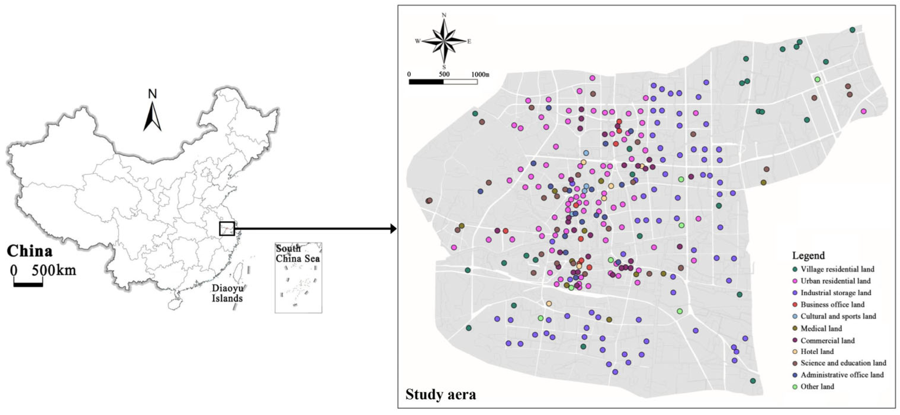
2.1. Study Area
2.2. Research Data
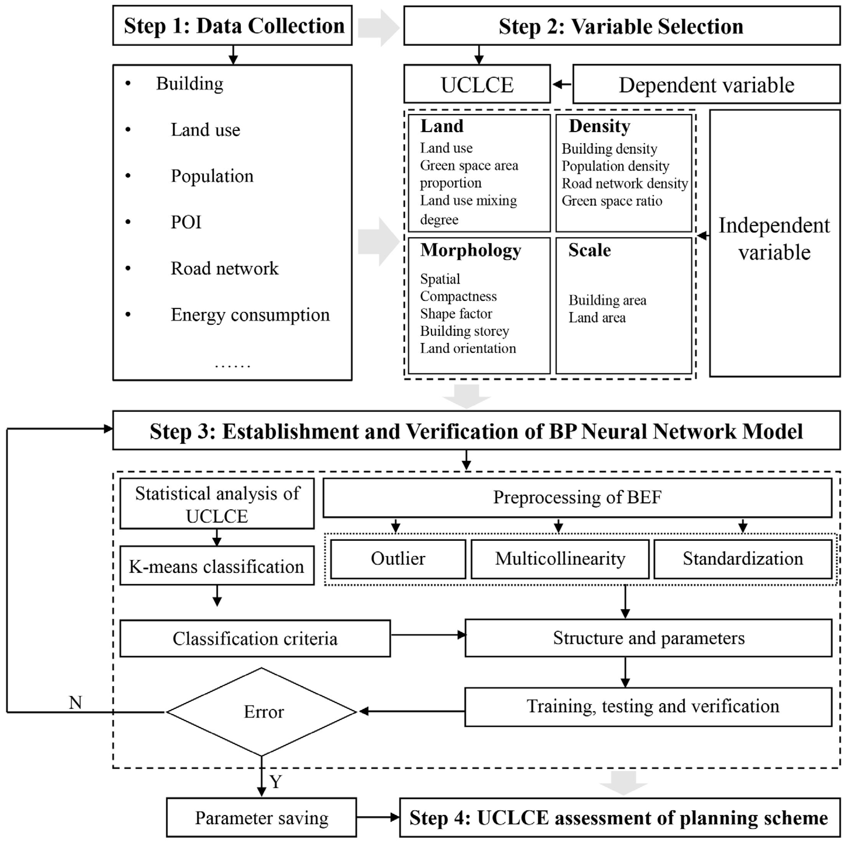
2.3. Methods
2.3.1. UCLCE Measurement Methods
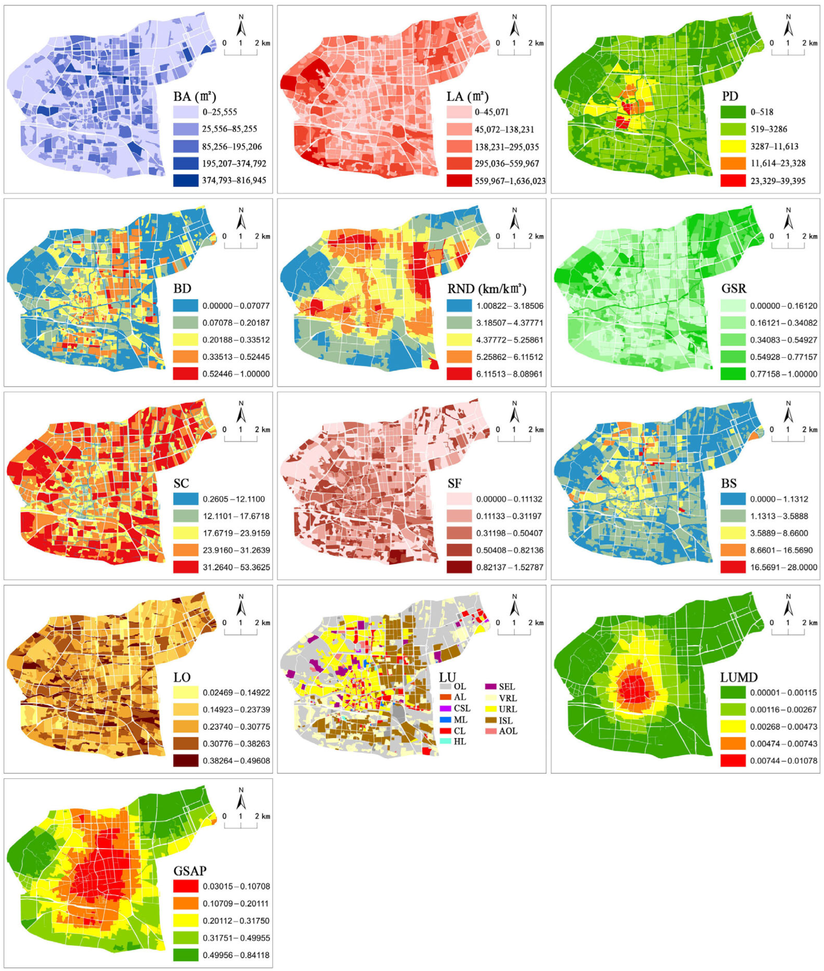
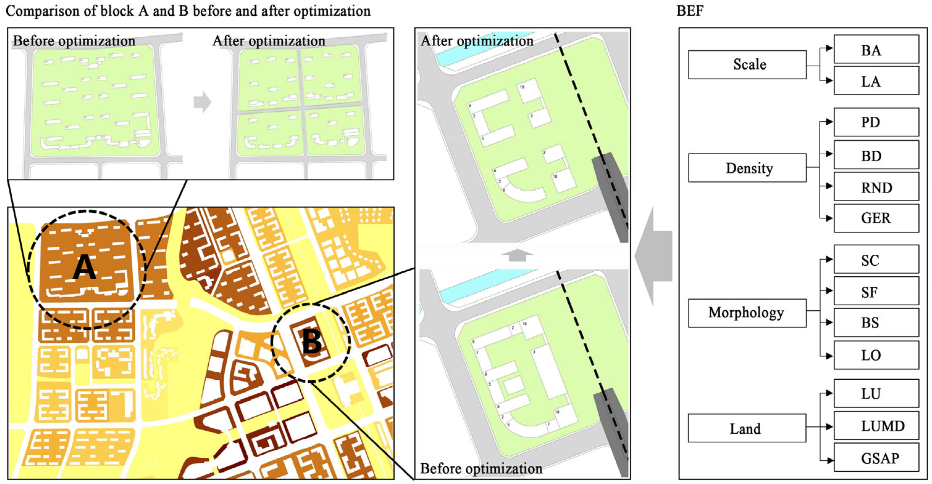
2.3.2. BEF Measurement Methods
2.3.3. BP Neural Network Model
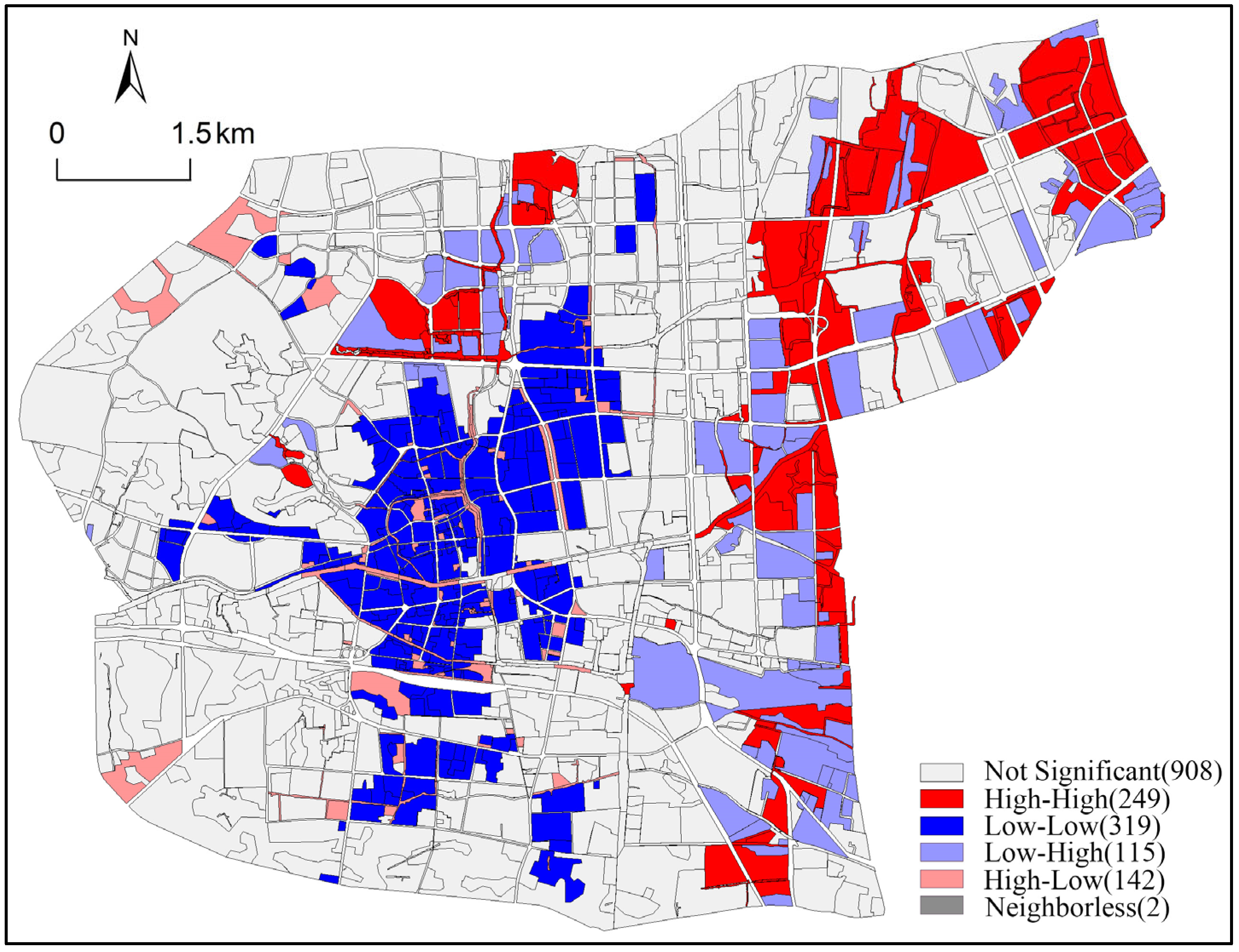
2.3.4. Spatial Autocorrelation of UCLCE
3. Results
3.1. Numerical Table of UCLCE
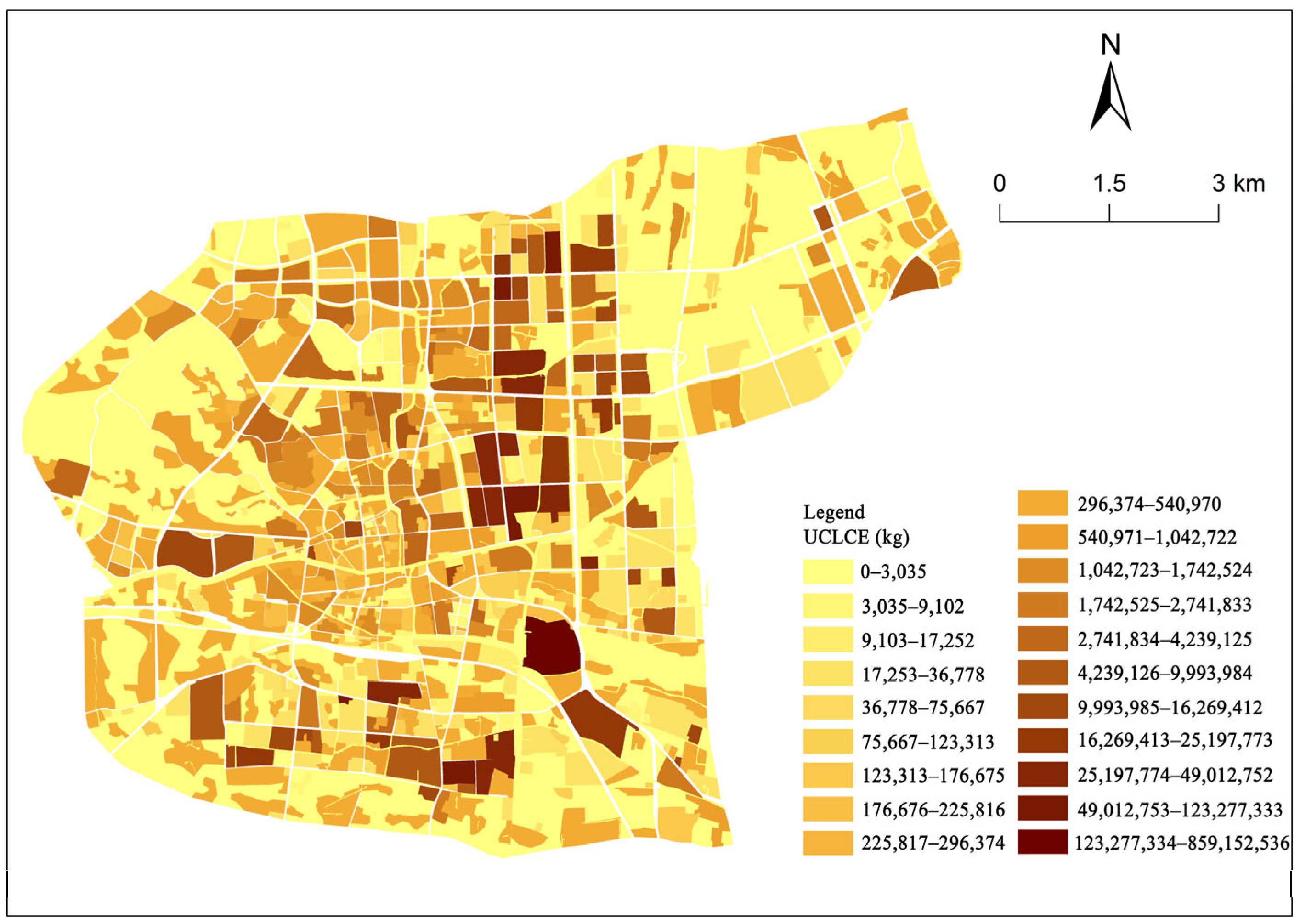
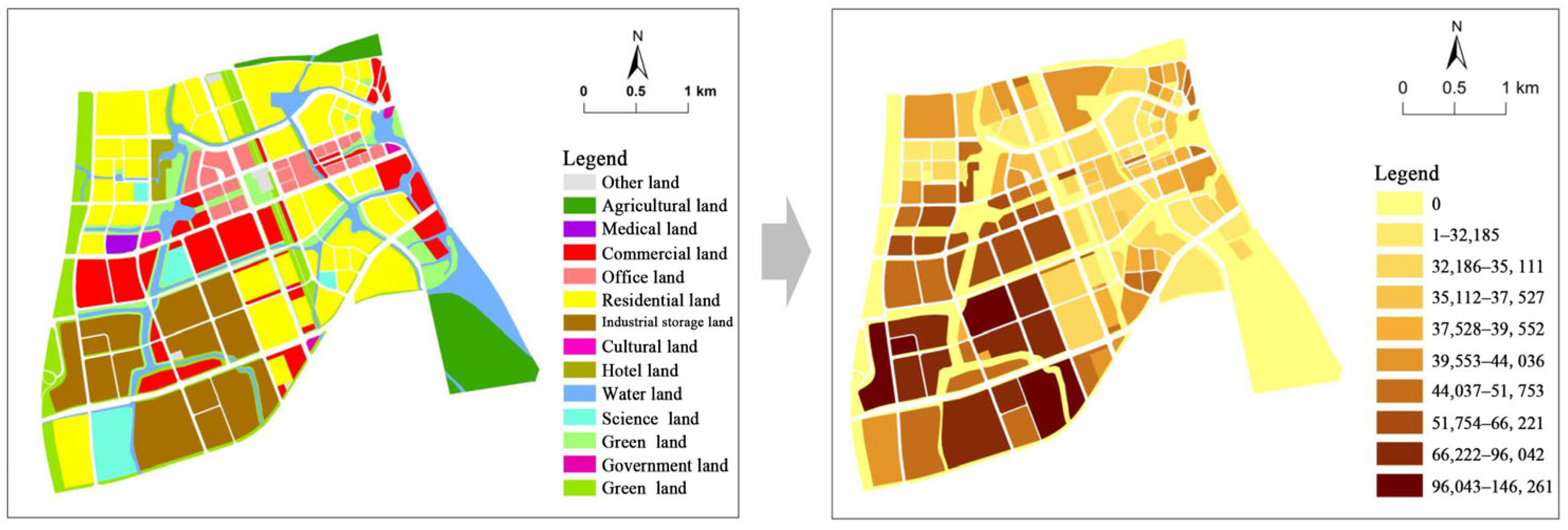
3.2. Spatial Distribution of UCLCE
3.3. Spatial Distribution of BEF
4. Discussions
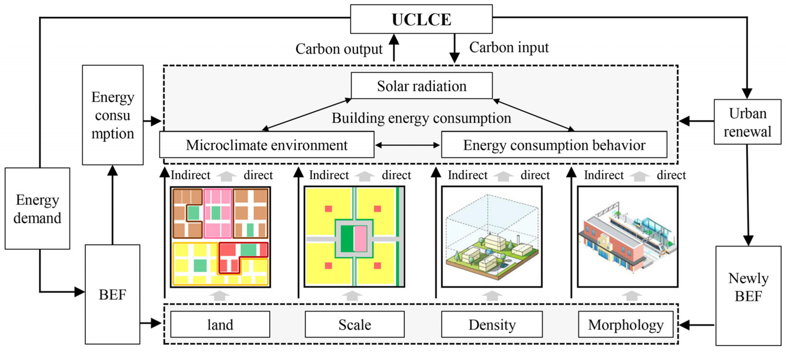
4.1. Influence Mechanism
4.1.1. UCL: The Spatial Carrier of Carbon Effects
4.1.2. Prediction Mechanism: BEF Impact Effect
4.2. Applications
4.3. Limitations and Further Improvements
4.3.1. Applicability and Limitations
4.3.2. Further Improvements
5. Conclusions
Author Contributions
Funding
Data Availability Statement
Conflicts of Interest
Abbreviations
| Full Name | Abbreviation |
| Urban Construction Land | UCL |
| Built Environment Elements | BEF |
| Ordinary Least Square | OLS |
| Urban Residential Land | URL |
| Business Office Land | BOL |
| Medical Land | ML |
| Hotel Land | HL |
| Administrative Office Land | AOL |
| Other Land | OL |
| Building Area | BA |
| Population Density | PD |
| Road Network Density | RND |
| Spatial Compactness | SC |
| Building Story | BS |
| Land Use | LU |
| Green Space Area Proportion | GSAP |
| Administrative Land | AL |
| Urban Construction Land Carbon Effects | UCLCE |
| Support Vector Machine | SVM |
| Village Residential Land | VRL |
| Industrial Storage Land | ISL |
| Cultural and Sports Land | CSL |
| Commercial Land | CL |
| Science and Education Land | SEL |
| Green Space Land | GSL |
| Point of Interest | POI |
| Land Area | LA |
| Building Density | BD |
| Green Space Ratio | GSR |
| Shape Factor | SF |
| Land Orientation | LO |
| Land Use Mixing Degree | LUMD |
| Residential Land | RL |
References
- Xu, Y.; Sun, L.; Wang, B.; Ding, S.M.; Ge, X.C.; Cai, S.R. Research on the Impact of Carbon Emissions and Spatial Form of Town Construction Land: A Study of Macheng, China. Land 2023, 12, 1385. [Google Scholar] [CrossRef]
- Zhang, X.P.; Liao, Q.H.; Yin, X.X.; Yin, Z.W.; Cao, Q.Q. Spatial Characteristics and Influencing Factors of Multi-Scale Urban Living Space (ULS) Carbon Emissions in Tianjin, China. Buildings 2023, 13, 2393. [Google Scholar] [CrossRef]
- Zhang, X.P.; Liao, Q.H.; Zhao, H.; Li, P. Vector maps and spatial autocorrelation of carbon emissions at land patch level based on multi-source data. Front. Public Health 2022, 10, 1006337. [Google Scholar] [CrossRef] [PubMed]
- Ou, Y.; Bao, Z.; Ng, S.T.; Song, W.; Chen, K. Land-use carbon emissions and built environment characteristics: A city-level quantitative analysis in emerging economies. Land Use Policy 2024, 137, 107019. [Google Scholar] [CrossRef]
- Liu, G.; Cui, F.; Wang, Y. Spatial effects of urbanization, ecological construction and their interaction on land use carbon emissions/absorption: Evidence from China. Ecol. Indic. 2024, 160, 111817. [Google Scholar] [CrossRef]
- Pu, J.; Xia, F. Exploring the relationship between city size and carbon emissions: An integrated population-land framework. Appl. Geogr. 2025, 177, 103571. [Google Scholar] [CrossRef]
- Zhang, X.; Zhang, D. Urban carbon emission scenario prediction and multi-objective land use optimization strategy under carbon emission constraints. J. Clean. Prod. 2023, 430, 139684. [Google Scholar] [CrossRef]
- Li, Y.; Peng, Y.-L.; Cheng, W.-Y.; Peng, H.-N. Spatial-temporal evolution and multi-scenario prediction of carbon emissions from land use in the adjacent areas of nature reserves. Ecol. Indic. 2025, 170, 113047. [Google Scholar] [CrossRef]
- Li, X.K.; Zhang, C.R.; Li, W.D.; Anyah, R.O.; Tian, J. Exploring the trend, prediction and driving forces of aerosols using satellite and ground data, and implications for climate change mitigation. J. Clean. Prod. 2019, 223, 238–251. [Google Scholar] [CrossRef]
- Qu, Y.; Zhan, L.; Zhang, Q.; Si, H.; Jiang, G. Towards sustainability: The impact of the multidimensional morphological evolution of urban land on carbon emissions. J. Clean. Prod. 2023, 424, 138888. [Google Scholar] [CrossRef]
- Svirejeva-Hopkins, A.; Schellnhuber, H.J. Urban expansion and its contribution to the regional carbon emissions: Using the model based on the population density distribution. Ecol. Model. 2008, 216, 208–216. [Google Scholar] [CrossRef]
- Chang, Y.; Xue, Y.; Song, S.; Geng, G. Analysis on carbon emission and peak forecasting of urban industrial zone renewal process in China based on extended Kaya identity. Energy 2025, 315, 134438. [Google Scholar] [CrossRef]
- Yang, Y.; Yang, M.; Zhao, B.; Lu, Z.; Sun, X.; Zhang, Z. Spatially explicit carbon emissions from land use change: Dynamics and scenario simulation in the Beijing-Tianjin-Hebei urban agglomeration. Land Use Policy 2025, 150, 107473. [Google Scholar] [CrossRef]
- Chuai, X.; Feng, J. High resolution carbon emissions simulation and spatial heterogeneity analysis based on big data in Nanjing City, China. Sci. Total Environ. 2019, 686, 828–837. [Google Scholar] [CrossRef]
- Lin, F.-Y.; Lin, T.-P.; Hwang, R.-L. Using geospatial information and building energy simulation to construct urban residential energy use map with high resolution for Taiwan cities. Energy Build. 2017, 157, 166–175. [Google Scholar] [CrossRef]
- Zhang, X.; Xie, Y.; Jiao, J.; Zhu, W.; Guo, Z.; Cao, X.; Liu, J.; Xi, G.; Wei, W. How to accurately assess the spatial distribution of energy CO2 emissions? Based on POI and NPP-VIIRS comparison. J. Clean. Prod. 2023, 402, 136656. [Google Scholar] [CrossRef]
- Al-Kabaha, Y.; Bataineh, K.; Aburabi’e, M. Multi-objective optimization of energy consumption, cost and emission for a residential building. Heliyon 2025, 11, e42139. [Google Scholar] [CrossRef]
- Eid, E.; Foster, A.; Alvarez, G.; Ndoye, F.-T.; Leducq, D.; Evans, J. Modelling energy consumption in a Paris supermarket to reduce energy use and greenhouse gas emissions using EnergyPlus. Int. J. Refrig. 2024, 168, 1–8. [Google Scholar] [CrossRef]
- Bahadori, E.; Rezaei, F.; He, B.-J.; Heiranipour, M.; Attia, S. Evaluating urban heat island mitigation strategies through coupled UHI and building energy modeling. Build. Environ. 2025, 280, 113111. [Google Scholar] [CrossRef]
- Zhang, L.; Sang, G.; Cui, X.; Han, W. Design optimization of rural building in dry-hot and dry-cold area using a back propagation (BP) neural network. Energy Build. 2022, 259, 111899. [Google Scholar] [CrossRef]
- Lei, R.; Yin, J. Prediction method of energy consumption for high building based on LMBP neural network. Energy Rep. 2022, 8, 1236–1248. [Google Scholar] [CrossRef]
- Zhang, L.; Sang, G.C.; Han, W.X. Effect of hygrothermal behaviour of earth brick on indoor environment in a desert climate. Sust. Cities Soc. 2020, 55, 102070. [Google Scholar] [CrossRef]
- Li, Q.D.; Sun, X.; Chen, C.; Yang, X.D. Characterizing the household energy consumption in heritage Nanjing Tulou buildings, China: A comparative field survey study. Energy Build. 2012, 49, 317–326. [Google Scholar] [CrossRef]
- Zhao, L.; Zhang, C.; Wang, Q.; Yang, C.; Zhou, W. Spatio-temporal variations of land use carbon emissions and its low carbon strategies for coastal areas in China with nighttime lighting data. J. Environ. Manag. 2025, 385, 125651. [Google Scholar] [CrossRef]
- Du, L.; Peng, C.; Ren, H.; Wu, Z.; Gao, W. Assessing Annual Carbon Emissions and its Peak Year in the Yangtze River Economic Belt (2021–2035) through Land Use/Land Cover Analysis. Sust. Cities Soc. 2025, 127, 106453. [Google Scholar] [CrossRef]
- Xu, C.G.; Xiong, W.; Zhang, S.M.; Shi, H.L.; Wu, S.C.; Bao, S.J.; Xiao, T.Q. Research on the Nonlinear Relationship Between Carbon Emissions from Residential Land and the Built Environment: A Case Study of Susong County, Anhui Province Using the XGBoost-SHAP Model. Land 2025, 14, 440. [Google Scholar] [CrossRef]
- Yu, Z.; Chen, L.; Tong, H.; Chen, L.; Zhang, T.; Li, L.; Yuan, L.; Xiao, J.; Wu, R.; Bai, L.; et al. Spatial correlations of land-use carbon emissions in the Yangtze River Delta region: A perspective from social network analysis. Ecol. Indic. 2022, 142, 109147. [Google Scholar] [CrossRef]
- Das, M.; Das, A. Dynamicity of carbon emission and its relationship with heat extreme and green spaces in a global south tropical mega-city region. Atmos. Pollut. Res. 2025, 16, 102484. [Google Scholar] [CrossRef]
- Wang, X.P.; Li, Z.Y.; Kee, T. Spatial and temporal correlation between green space landscape pattern and carbon emission-Three major coastal urban agglomerations in China. Urban Clim. 2024, 58, 102222. [Google Scholar] [CrossRef]
- Bai, J.; Chen, H.; Gu, X.; Ji, Y.; Zhu, X. Temporal and spatial characteristics of carbon emissions from cultivated land use and their influencing factors: A case study of the Yangtze River Delta region. Int. Rev. Econ. Financ. 2024, 96, 103501. [Google Scholar] [CrossRef]
- Zhao, Q.Y.; Xie, B.Y.; Han, M.Y. Unpacking the Sub-Regional Spatial Network of Land-Use Carbon Emissions: The Case of Sichuan Province in China. Land 2023, 12, 1927. [Google Scholar] [CrossRef]
- Luo, Z.X.; Yang, L.; Liu, J.P. Embodied carbon emissions of office building: A case study of China’s 78 office buildings. Build. Environ. 2016, 95, 365–371. [Google Scholar] [CrossRef]
- Wang, L.; Chen, T.; Yu, Y.; Wang, L.Y.; Zang, H.Y.; Cang, Y.; Zhang, Y.O.; Ma, X.W. Impacts of Vegetation Ratio, Street Orientation, and Aspect Ratio on Thermal Comfort and Building Carbon Emissions in Cold Zones: A Case Study of Tianjin. Land 2024, 13, 1275. [Google Scholar] [CrossRef]
- Wang, L. Assessment of land use change and carbon emission: A Log Mean Divisa (LMDI) approach. Heliyon 2024, 10, e25669. [Google Scholar] [CrossRef] [PubMed]
- Shi, Y.S.; Zheng, B.; Wang, Z.; Zheng, J.W. Mixed Land Use and Its Relationship with CO2 Emissions: A Comparative Analysis Based on Several Typical Development Zones in Shanghai. Land 2023, 12, 1675. [Google Scholar] [CrossRef]
- Ji, R.R.; Wang, K.; Zhou, M.R.; Zhang, Y.; Bai, Y.J.; Wu, X.; Yan, H.; Zhao, Z.Q.; Ye, H. Green Space Compactness and Configuration to Reduce Carbon Emissions from Energy Use in Buildings. Remote Sens. 2023, 15, 1502. [Google Scholar] [CrossRef]
- Luo, H.; Zhang, Y.; Gao, X.; Liu, Z.; Song, X.; Meng, X.; Yang, X. Unveiling land use-carbon Nexus: Spatial matrix-enhanced neural network for predicting commercial and residential carbon emissions. Energy 2024, 305, 131722. [Google Scholar] [CrossRef]
- Zhang, M.; Kafy, A.A.; Xiao, P.; Han, S.; Zou, S.; Saha, M.; Zhang, C.; Tan, S. Impact of urban expansion on land surface temperature and carbon emissions using machine learning algorithms in Wuhan, China. Urban Clim. 2023, 47, 101347. [Google Scholar] [CrossRef]
- Tian, D.; Zhang, J.; Li, B.; Xia, C.; Zhu, Y.; Zhou, C.; Wang, Y.; Liu, X.; Yang, M. Spatial analysis of commuting carbon emissions in main urban area of Beijing: A GPS trajectory-based approach. Ecol. Indic. 2024, 159, 111610. [Google Scholar] [CrossRef]
- Zhou, Y.; Hu, D.; Wang, T.; Tian, H.; Gan, L. Decoupling effect and spatial-temporal characteristics of carbon emissions from construction industry in China. J. Clean. Prod. 2023, 419, 138243. [Google Scholar] [CrossRef]
- Freitas, W.W.L.; de Souza, R.M.C.R.; Amaral, G.J.A.; Bastiani, F.D. Exploratory spatial analysis for interval data: A new autocorrelation index with COVID-19 and rent price applications. Expert Syst. Appl. 2022, 195, 116561. [Google Scholar] [CrossRef]
- Mtshawu, B.; Bezuidenhout, J.; Kilel, K.K. Spatial autocorrelation and hotspot analysis of natural radionuclides to study sediment transport. J. Environ. Radioact. 2023, 264, 107207. [Google Scholar] [CrossRef]
- Gedamu, W.T.; Plank-Wiedenbeck, U.; Wodajo, B.T. A spatial autocorrelation analysis of road traffic crash by severity using Moran’s I spatial statistics: A comparative study of Addis Ababa and Berlin cities. Accid. Anal. Prev. 2024, 200, 107535. [Google Scholar] [CrossRef]
- Li, W.Y.; Wang, K.Q.; Liu, H.M.; Zhang, Y.X.; Zhu, X.D. Construction Land Transfer Scale and Carbon Emission Intensity: Empirical Evidence Based on County-Level Land Transactions in Jiangsu Province, China. Land 2024, 13, 917. [Google Scholar] [CrossRef]
- Fang, Y.; Zhao, L. Exploring the decoupling effect and driving mechanism of carbon emissions at macroscale: An empirical study from Wuhan metropolitan area. Urban Clim. 2025, 61, 102434. [Google Scholar] [CrossRef]
- Lin, Q.W.; Zhang, L.; Qiu, B.K.; Zhao, Y.; Wei, C. Spatiotemporal Analysis of Land Use Patterns on Carbon Emissions in China. Land 2021, 10, 141. [Google Scholar] [CrossRef]
- Wu, Z.H.; Zhou, L.H.; Wang, Y.B. Prediction of the Spatial Pattern of Carbon Emissions Based on Simulation of Land Use Change under Different Scenarios. Land 2022, 11, 1788. [Google Scholar] [CrossRef]
- Wang, C.; Yang, Y.J.; Bai, Y.P.; Teng, Y.M.; Zhan, J.Y. Land use data can improve the accuracy of carbon emission spatial inversion model. Land Degrad. Dev. 2024, 35, 2345–2366. [Google Scholar] [CrossRef]
- Li, Z.; Sun, H.; Long, J.; Qiu, S. Study on the matching characteristics between office building energy consumption and rooftop photovoltaics in regions with hot summers and cold winters. Renew. Energy 2025, 249, 123285. [Google Scholar] [CrossRef]
- Kaloop, M.R.; Ahmad, F.; Samui, P.; Elbeltagi, E.; Hu, J.-W.; Wefki, H. Predicting energy consumption of residential buildings using metaheuristic-optimized artificial neural network technique in early design stage. Build. Environ. 2025, 274, 112749. [Google Scholar] [CrossRef]
- Delmastro, C.; Mutani, G.; Pastorelli, M.; Vicentini, G. Urban morphology and energy consumption in Italian residential buildings. In Proceedings of the 2015 International Conference on Renewable Energy Research and Applications (ICRERA), Palermo, Italy, 22–25 November 2015. [Google Scholar]
- Li, Z.W.; Dai, J.; Chen, H.Z.; Lin, B.R. An ANN-based fast building energy consumption prediction method for complex architectural form at the early design stage. Build. Simul. 2019, 12, 665–681. [Google Scholar] [CrossRef]
- Wang, P.; Yang, Y.T.; Ji, C.; Huang, L. Positivity and difference of influence of built environment around urban park on building energy consumption. Sust. Cities Soc. 2023, 89, 104321. [Google Scholar] [CrossRef]
- Dujardin, S.; Marique, A.F.; Teller, J. Spatial planning as a driver of change in mobility and residential energy consumption. Energy Build. 2014, 68, 779–785. [Google Scholar] [CrossRef]


| Name | Description | Sources |
|---|---|---|
| Industrial POI data | Industrial storage land patch spatial location dataset | Baidu map |
| Road systems of Changxing | Vector data of road traffic system | Department of Transportation |
| Land use map of Changxing | Vector map of different land use types | Natural Resources Bureau |
| Urban population data | Population of urban residential lands | Public Security Bureau |
| Rural population data | Population of rural residential lands | Public Security Bureau |
| Architecture data | Building outline contains name, number, height, area, perimeter, and floor information | Construction Bureau |
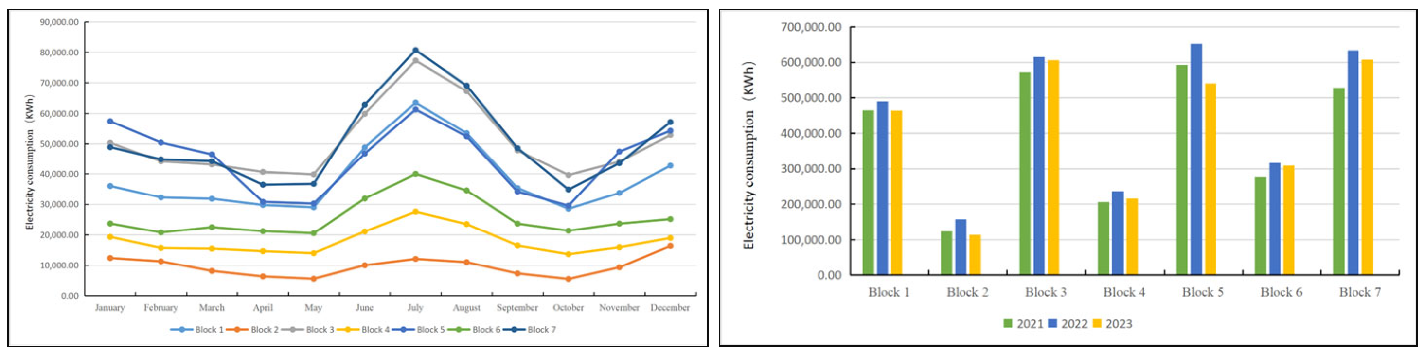
| Electricity consumption data | Electricity consumption of Changxing | Statistics Bureau |
| Type | BEF | Formula | Description | Source |
|---|---|---|---|---|
| Scale | Building area (BA) | (i = 1, 2, …, n) | is the building base area of the i-th building, m2; is the number of floors of the i-th building; represents the number of buildings on the block | [24] |
| Land area (LA) | (i = 1, 2, …, n) | is the area of the land of Type i, which is automatically extracted in GIS | [8] | |
| Density | Population density (PD) | is the number of people accommodated on the block; is the land area | [6,25] | |
| Building density (BD) | (i = 1, 2, … n) | is the base area of the i-th building on the land. is the land area; represents the number of buildings on the block | [26] | |
| Road network density (RND) | (i = 1, 2, … n) | is the length of the i-th section of the road within a 1000 m range of the land. represents the area within a 1000 m range of the land. represents the number of road sections | [27] | |
| Green space ratio (GSR) | (i = 1, 2, …, n) | is the green space area of the i-th block; is the area of the i-th block | [28,29] | |
| Morphology | Spatial Compactness (SC) | represents the area of the land use; is the perimeter of the land use | [30] | |
| Shape factor (SF) | (i = 1, 2, …, m) | represents the number of buildings on the block. is the i-th building; represents the number of building floors; represents the floor height of the building; is the width of the bottom surface of the building; is the length of the bottom surface of the building; represents the floor area of the building | [31] | |
| Building storey (BS) | (i = 1, 2, …, n) | is the building area on the block; is the base area of the i-th building on the land. represents the number of buildings on the block | [32] | |
| Land orientation (LO) | (i = 1, 2, …, n) | is the southbound length of the i-th block; is the perimeter of the i-th block | [33] | |
| Land | Land use (LU) | (i = 1, 2, …, 11) | is the function of block i. 1 is VRL. 2 is URL. 3 is ISL. 4 is BOL. 5 is CSL. 6 is ML. 7 is CL. 8 is HL. 9 is SEL. 10 is AOL. 11 is OL. | [34] |
| Land use mixing degree (LUMD) | (j = 1, 2, …, n) | is the proportion of the area of Class i land within a 1000 m range of the land use. represents the quantity of building land types within a 1000 m range of the land | [35] | |
| Green space area proportion (GSAP) | (i = 1, 2,…, n) | is the area of the i-th green space within a 1000 m range of the land use. represents the area within a 1000 m range of the land. represents the number of green space | [36] |
| Parameters | Value |
|---|---|
| net. trainParam. epochs | 10,000 |
| net. trainParam. goal | 0.001 |
| net. trainParam. lr | 0.8 |
| net. trainParam. mc | 0.6 |
| net. trainParam. max_fail | 10,000 |
| net. trainParam. mem_reduc | 3 |
| net. trainParam. show | 100 |
| Type | Mean Total Effect (kgCO2/m2) | Mean Intensity Effect (kgCO2/m2) |
|---|---|---|
| RL | 760,601.25 | 12.76 |
| ISL | 6,346,118.38 | 86.99 |
| AL | 175,911.9 | 12.40 |
| SEL | 586,458.01 | 8.43 |
| ML | 1,201,185.03 | 65.99 |
| CL | 554,470.07 | 28.93 |
| OL | 2,011,613.45 | 16.87 |
Disclaimer/Publisher’s Note: The statements, opinions and data contained in all publications are solely those of the individual author(s) and contributor(s) and not of MDPI and/or the editor(s). MDPI and/or the editor(s) disclaim responsibility for any injury to people or property resulting from any ideas, methods, instructions or products referred to in the content. |
© 2025 by the authors. Licensee MDPI, Basel, Switzerland. This article is an open access article distributed under the terms and conditions of the Creative Commons Attribution (CC BY) license (https://creativecommons.org/licenses/by/4.0/).
Share and Cite
Liao, Q.; Zhang, X.; Cui, Z.; Yin, X. Prediction of Urban Construction Land Carbon Effects (UCLCE) Using BP Neural Network Model: A Case Study of Changxing, Zhejiang Province, China. Buildings 2025, 15, 2312. https://doi.org/10.3390/buildings15132312
Liao Q, Zhang X, Cui Z, Yin X. Prediction of Urban Construction Land Carbon Effects (UCLCE) Using BP Neural Network Model: A Case Study of Changxing, Zhejiang Province, China. Buildings. 2025; 15(13):2312. https://doi.org/10.3390/buildings15132312
Chicago/Turabian StyleLiao, Qinghua, Xiaoping Zhang, Zixuan Cui, and Xunxi Yin. 2025. "Prediction of Urban Construction Land Carbon Effects (UCLCE) Using BP Neural Network Model: A Case Study of Changxing, Zhejiang Province, China" Buildings 15, no. 13: 2312. https://doi.org/10.3390/buildings15132312
APA StyleLiao, Q., Zhang, X., Cui, Z., & Yin, X. (2025). Prediction of Urban Construction Land Carbon Effects (UCLCE) Using BP Neural Network Model: A Case Study of Changxing, Zhejiang Province, China. Buildings, 15(13), 2312. https://doi.org/10.3390/buildings15132312