Abstract
During the cantilever casting construction process of continuous girder bridges, it is crucial to accurately predict the pre-camber of each cantilever segment to ensure smooth closure of the bridge, structural safety, and construction quality. However, traditional methods for predicting pre-camber have limited accuracy and primarily handle linear relationships. Therefore, this paper proposes a pre-camber prediction model based on a Convolutional-Bidirectional Long Short-Term Memory network with a fusion attention mechanism (CNN-BiLSTM-Attention) and utilizes the Dung Beetle Optimizer (DBO) algorithm to optimize the hyperparameters of the CNN-BiLSTM-Attention model to enhance its predictive performance. The research results indicate that compared to several other prediction models, the model proposed in this paper demonstrates superior performance in predicting the pre-camber of continuous girder bridges. Compared to other prediction models, the evaluation metrics MAE, RMSE, and MAPE of the model proposed in this paper are minimized to 2.76 mm, 3.47 mm, and 0.70%, respectively. Applying the model proposed in this paper to the cantilever casting stage of the elevated continuous girder bridges in Shenyang Metro, China, enables pre-camber prediction with an accuracy of an average absolute error of less than 2 mm, providing a new efficient method for pre-camber prediction in cantilever casting construction.
1. Introduction
The construction of cantilever casting for long-span continuous girder bridges is a lengthy and complex process. During the construction process, factors such as the self-weight of cantilever casting segments, temperature variations, changes in construction loads, errors in prestressing force application, concrete shrinkage and creep, as well as transitions in structural systems, all significantly affect the alignment of bridge structures [1,2,3,4]. Therefore, during the cantilever casting construction of the main girder, it is usually necessary to establish a certain amount of pre-camber to counteract the various deformations that occur during construction and to provide the necessary deflection reserve for the completed bridge. To ensure that the cantilever casting construction ultimately achieves perfect alignment of the bridge and that the alignment of the bridge structure meets design requirements after construction, the precise prediction of the pre-camber is necessary to control the alignment of the bridge’s main structure [5,6,7,8,9].
Currently, the prediction of bridge pre-camber typically utilizes methods such as grey theory, Kalman filtering, and least squares. While these methods are widely used for predicting and adjusting bridge pre-camber, they have drawbacks, including a high workload, a capability limited to linear relationships, and consideration of only a small number of parameters [10,11,12,13]. In recent years, with the rapid development of artificial intelligence technology, artificial neural networks have been increasingly applied in civil engineering and have gradually demonstrated their unique advantages [14,15,16,17]. These advantages include, but are not limited to, the ability to handle complex nonlinear problems, extract key information from large datasets, and adapt to environmental changes through self-learning. In civil engineering practice, the application of artificial neural networks has expanded to various aspects such as predicting structural parameters, evaluating structural system performance, and recognition [18,19,20]. With the development of intelligent algorithms, data-driven neural networks and machine learning methods are gradually being applied to bridge engineering, bringing new momentum to the control of bridge construction alignment [21,22,23].
2. Literature Review
Long Short-Term Memory networks (LSTM) are among the crucial frameworks of neural networks. Due to their unique memory capabilities and gate structure, they can simultaneously consider the temporal nature and non-linearity of multidimensional data, making them widely applicable in the prediction domain. Shan [24] proposed an innovative deformation prediction framework that integrates spatiotemporal clustering algorithms, Empirical Mode Decomposition (EMD), and Long Short-Term Memory (LSTM) networks. Through experiments conducted on large excavation pits, this method significantly enhances the accuracy and efficiency of predicting large-scale structural deformations. Xu [25] presented a recursive Long Short-Term Memory (LSTM) neural network aimed at forecasting non-linear structural seismic responses with varying lengths and sampling frequencies. This recursive LSTM framework is capable of accurately capturing both overarching and intricate temporal features across diverse datasets of structural responses, exhibiting strong precision and generalization prowess. However, a single LSTM has certain limitations in extracting spatial features, which results in an inadequate capability to suppress random interference and extract spatial local information. Therefore, it is necessary to optimize it or use it in conjunction with other algorithms to further improve prediction accuracy.
Due to the powerful feature extraction capability of Convolutional Neural Networks (CNN), they are widely applied in fields such as life prediction and fault diagnosis. Li et al. [26] proposed a multi-scale feature extraction strategy based on stacked CNN using deep learning to achieve high accuracy in predicting remaining useful life. Hu [27] proposed a method using a Convolutional Neural Network (CNN) and autoencoders to predict bridge pattern shapes. Despite CNNs’ ability to automatically extract multidimensional spatial features from large datasets, their capability to handle time-dependent sequential data is relatively weak. In contrast, LSTMs effectively address long-term dependency issues by introducing gating units. Combining CNNs and LSTMs enhances the extraction of spatial and temporal features, addressing long-term dependencies while reducing computational time. Elmaz et al. [28] established a CNN-LSTM model using convolutional layers as feature extractors for raw data, feeding the output into LSTM to accurately predict indoor temperatures. Wang et al. [29] integrated the spatial dependencies of track geometry shapes across adjacent sections using CNN, utilized LSTM to learn the dynamic changes of trajectory geometry data over time, considering the temporal dependencies of trajectory geometry data, and achieved good predictive results for railway track geometry changes. Bidirectional LSTM networks (BiLSTMs) extend traditional unidirectional LSTMs by learning bidirectional features, thereby further improving the model’s prediction accuracy. Méndez et al. [30] proposed a hybrid model CNN-BiLSTM that combines a Convolutional Neural Network with Bidirectional LSTM and applied it to long-term urban traffic flow prediction. The research results indicated that the BiLSTM network outperformed LSTM networks in time-series tasks. The above studies demonstrate the effectiveness of CNN-BiLSTM algorithms in prediction tasks, yet their direct application to the field of bridge construction control remains underexplored.
Addressing the aforementioned issues, this paper combines CNN and BiLSTM, integrating an Attention mechanism to extract crucial information, to establish a model for predicting pre-camber in cantilever construction. Utilizing CNN’s spatial feature extraction capability to extract correlations between various parameters during cantilever construction, leveraging BiLSTM to effectively capture long-term dependencies in the data bidirectionally, better understanding data-related features in cantilever construction and the overall impact of preceding and succeeding data. The addition of an Attention mechanism focuses the model on the patterns of feature changes in the data, enhancing the understanding of internal correlations in sequential data. The Dung Beetle Optimizer (DBO) algorithm adjusts multiple hyperparameters of the CNN-BiLSTM-Attention model to find an optimal combination for the current task and dataset, thereby improving predictive performance and achieving accurate pre-camber prediction during cantilever construction. Finally, the applicability and accuracy of this method were validated through application to an actual continuous girder bridge, and the performance of the predictive model was evaluated based on evaluation criteria.
3. Design of the DBO-CNN-LSTM-Attention Neural Network Model
3.1. Convolutional Neural Network (CNN)
The Convolutional Neural Network (CNN), introduced by Lecun et al. in 1998, represents a distinct variant of feedforward neural networks. Its architecture encompasses convolutional layers, pooling layers, and fully connected layers, exhibiting characteristics such as local connectivity and weight sharing, as illustrated in Figure 1 [31]. Within the convolutional layer, convolution operations are executed on multi-feature input data utilizing kernels to extract pertinent features. Subsequently, the pooling layer reduces the dimensionality of the input data, thereby decreasing computational load while retaining crucial features. Ultimately, the fully connected layer integrates the outputs from both the convolutional and pooling layers to produce the ultimate classification outcomes or regression values [32]. The training process of CNN typically uses a backpropagation algorithm to update weight parameters. The convolutional layer calculation formula is as follows:
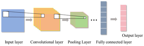
Figure 1.
CNN structure.
In the formula, represents the input of the j-th convolution kernel in the lth layer, which is also the output of the l−1-th layer; denotes the activation function; denotes the set of input mapping layers; denotes the weight matrix of the j-th convolution kernel in the l-th layer; and denotes the bias term.
The pooling layer reduces the dimensionality of the convolutional layer’s output through methods like max pooling and average pooling to facilitate feature extraction.
The fully connected layer concatenates the output results of the pooling layer and outputs these concatenated feature vectors to the classifier. The forward propagation output of the fully connected layer is:
In the formula, represents the value of the j-th output neuron in the l+1-th layer.
3.2. BiLSTM Network
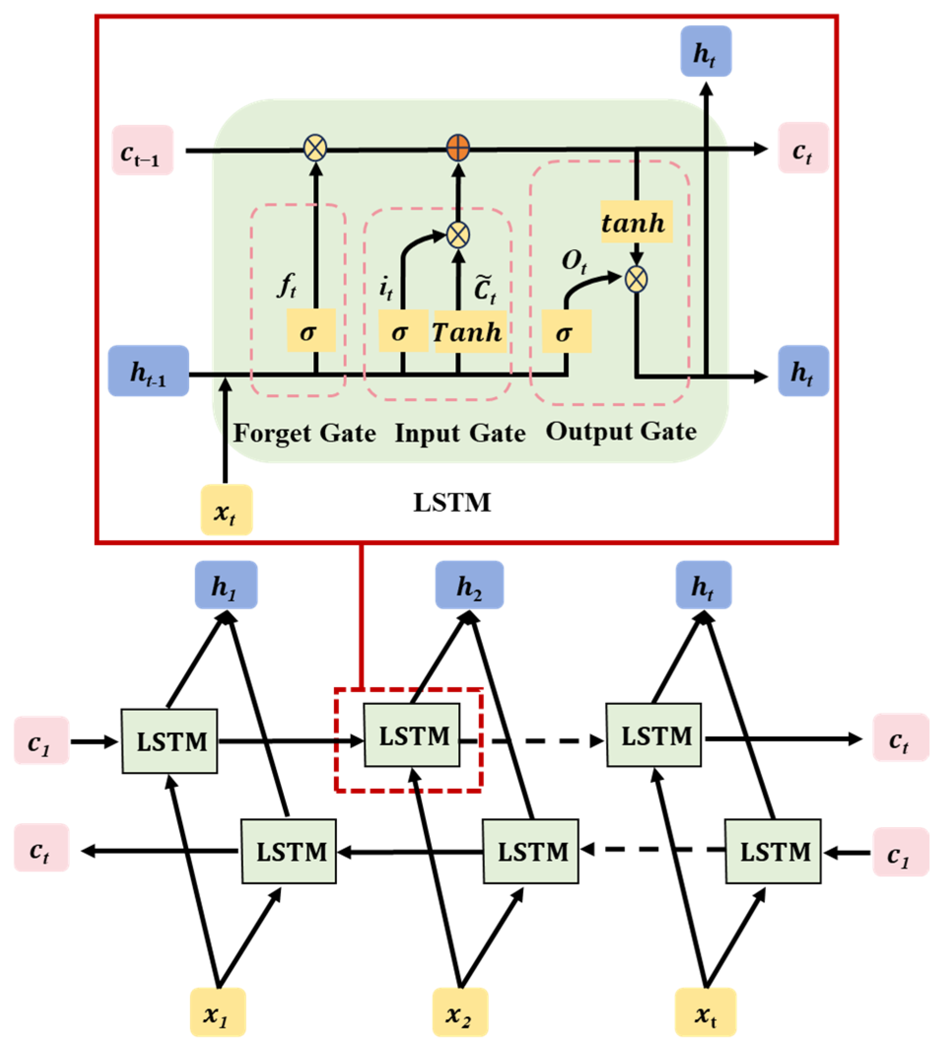
Long Short-Term Memory (LSTM) networks represent an advanced form of Recurrent Neural Networks (RNNs), extensively employed for the analysis of sequential data [33]. In contrast to conventional RNNs, LSTMs excel at capturing long-range dependencies within sequences and alleviating problems such as vanishing or exploding gradients. This enhanced capability stems from the incorporation of gating mechanisms, comprising forget gates, input gates, output gates, and a memory cell. These gates regulate the movement of information, enabling LSTMs to selectively preserve or disregard information during sequence processing. By leveraging this gating architecture, LSTMs achieve greater flexibility in capturing long-term dependencies within sequential data and effectively tackle the challenges posed by vanishing or exploding gradients. The internal configuration of LSTM units is depicted in Figure 2. The detailed mathematical expressions underpinning LSTM network operations are provided as follows:
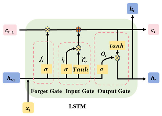
Figure 2.
Internal structure of LSTM unit.
In the formula: , , , denote the weight matrices corresponding to ; , , , denote the weight matrices of ; , , , denote the bias vectors; and tanh() denotes the activation function.
BiLSTM (Bidirectional Long Short-Term Memory) is an extension of the traditional LSTM (Long Short-Term Memory) neural network, as illustrated in Figure 3. By introducing bidirectional processing, BiLSTM expands the capabilities of LSTM networks, enabling them to capture contextual information from past and future data points in sequences [34]. Processing sequences with bidirectional information flow allows BiLSTM to comprehensively capture contextual information from both the past and future, making it particularly suitable for tasks requiring consideration of a global context. Compared to traditional LSTM, BiLSTM more effectively captures long-term dependencies in sequences, offering better performance for tasks requiring long-term memory. At each time step, BiLSTM integrates past and future information simultaneously, enhancing the flexibility of information flow. In the cantilever casting construction process, various factors have long-term effects on the pre-camber, such as the length of concrete segment casting, the concrete modulus of elasticity, and the concrete density. Setting the pre-camber before casting each segment requires consideration of its impact on the linearity of the construction process before and after. BiLSTM can effectively capture these influences, thereby assisting in optimizing the setting of the pre-camber to better align with actual construction conditions and improve engineering quality and efficiency.

Figure 3.
BiLSTM neural network structure.
3.3. Attention Mechanism
In order to prevent the model from ignoring crucial parts of the data during computation, which could lead to information loss, the Attention mechanism is introduced to selectively focus on different levels of data, prioritizing highly weighted and relevant information, while assigning lower weights to less distinctive features. This facilitates a deeper feature extraction process for the data, thereby reducing errors in multi-step predictions [35]. The Attention mechanism allows the model to flexibly focus on important parts when processing sequential data, thereby enhancing the model’s performance and effectiveness. The Attention mechanism scores the hidden unit ht using the softmax function, with the scoring calculated as follows:
In the equation, represents the similarity score, indicating the correlation between historical state ht and the output state. is the weight matrix, is the bias term, and represents the attention weight of ht, indicating the importance of this historical state. Assigning attention weights to each historical state, we obtain the optimized output result h through weighted averaging:
3.4. DBO Algorithm
3.4.1. Principle and Process of DBO Algorithm
The Dung Beetle Optimization (DBO) algorithm draws inspiration from the natural behaviors of dung beetles, offering distinct advantages over conventional optimization techniques like the Genetic Algorithm, Particle Swarm Optimization, and Ant Colony Optimization. These advantages include rapid convergence, high precision, and stability [36]. Unlike these traditional methods, DBO achieves global optimization by mimicking the behaviors of dung beetles, such as rolling balls, dancing, foraging, stealing, and reproducing, to pinpoint the optimal position. Notably, in open environments, dung beetles rely on the sun for navigation while rolling their dung balls. The influence of sunlight on their rolling positions results in updated positions for the dung balls, which can be mathematically represented as follows:
In the equation, t represents the number of iterations; represents the position information of the i-th beetle in the t-th iteration; k is the disturbance coefficient ; b is a constant value ranging from ; a represents the positional deviation of beetles due to natural factors, taking a value of either −1 or 1 (1 indicates no deviation, −1 indicates deviation direction); XW represents the worst position in the global context; and Δx represents the change in light intensity, where a larger value indicates weaker light.
When a dung beetle is obstructed and unable to proceed, it repositions its path through dance behaviors. Therefore, simulating dung beetle’s dance behavior with a tangent function yields a new path, considering only the interval [0, π] for the domain. Once the dung beetle determines a new direction, it continues to move, updating its position to:
In the equation, θ represents the disturbance angle, ranging from [0, π]. If θ takes values of 0, π/2, or π, the position of the beetle is not updated.
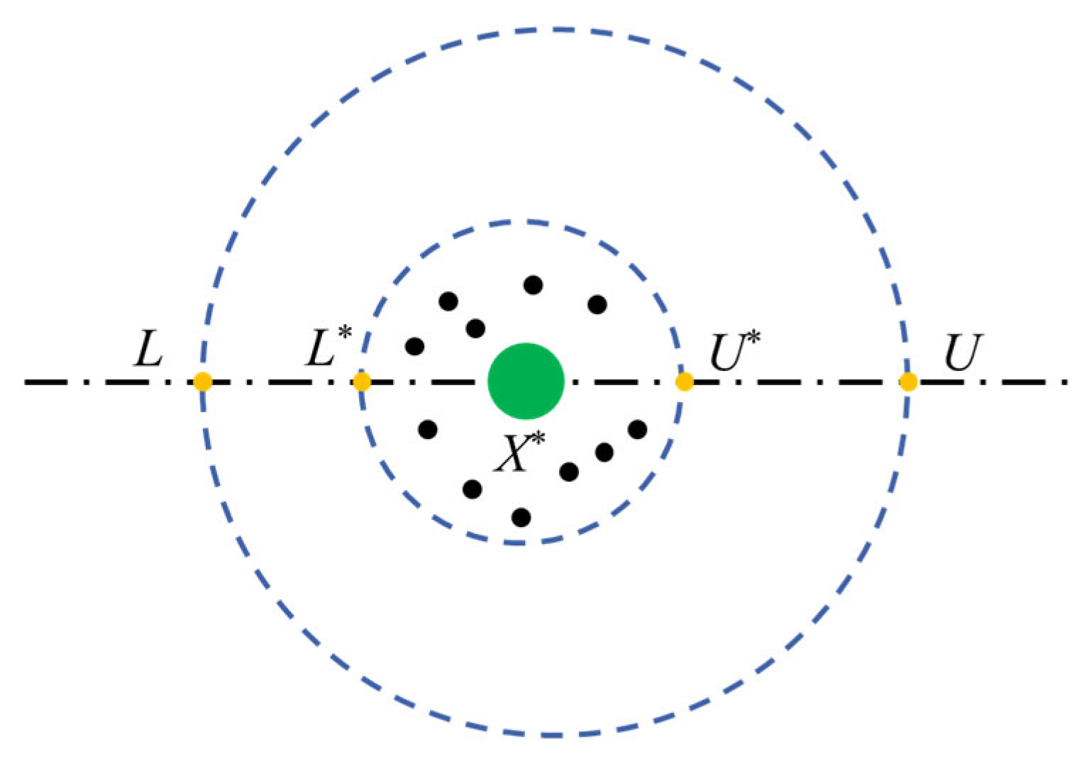
In nature, beetles select appropriate oviposition sites crucial for the safe reproduction of their offspring. The boundary selection strategy for oviposition by female beetles is represented as [36]:
In the equation, L∗ is the upper boundary of the oviposition area; U∗ is the lower boundary of the oviposition area; X∗ represents the local optimal position; L is the upper bound of the optimization problem; U is the lower bound of the optimization problem; and Tmax is the maximum number of iterations.
As shown in Figure 4, the green circle represents the current local optimal position, surrounded by dots representing eggs, each containing a beetle egg. The blue color indicates the upper and lower boundaries. Once the oviposition area is determined, female beetles will lay eggs in this area. In the DBO algorithm, each female beetle lays only one egg. Furthermore, the boundary range of the oviposition area is dynamically changing, leading to dynamic changes in the position of the eggs during iterations, represented as:
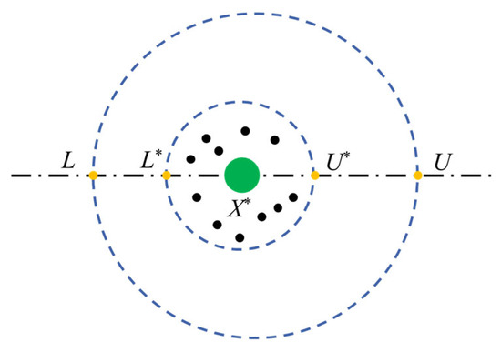
Figure 4.
Boundary selection strategy.
In the equation, Bi(t) represents the position of the i-th egg during the t-th iteration; b1 and b2 denote two independent vectors of size 1 × D, where D represents the optimization dimension.
Since some mature beetles need to emerge from the ground to forage, it is necessary to establish an optimal foraging area to guide beetle foraging, with the optimal foraging area boundaries as:
In the equation, Lb represents the lower boundary of the optimal foraging area; Xb represents the globally optimal foraging position; and Ub represents the upper boundary of the optimal foraging area.
Thus, the updated position of the small beetles is:
where xi(t) represents the position of the i-th small beetle in the t-th iteration; C1 denotes a random number following a normal distribution; and C2 denotes a random vector from (0, 1).
Some beetles are also known as thieves, which steal food from other beetles. From Equation (19), it is known that Xb is the best food source location; thus, Xb can be designated as the optimal food stealing location. During iterations, the position of the thieves is:
In the equation, xi(t) represents the position of the i-th thief in the t-th iteration; g denotes a random vector of size 1 × D following a normal distribution; S represents a constant value; and as thieves continuously update, the final optimal position output is Xb.
Formula (19) details the position-update mechanism of thieves in the Dung Beetle Optimization (DBO) algorithm: This formula uses the current global optimal food position as the core anchor point. By introducing a random vector following a normal distribution (providing an exploration direction) and a constant step-size factor (controlling the movement amplitude), it drives the thieves to move towards the optimal region. Simultaneously, a self-adaptive adjustment factor, composed of the distance terms (distance to the local optimal position) and (distance to the global optimal position), enables the thieves to dynamically adjust their movement step-size based on the spatial relationship between their current position and high-quality solutions. When far from high-quality solutions, they take larger steps to accelerate convergence; when close to high-quality solutions, they fine-tune the step-size for a granular search. Ultimately, this achieves a balance between exploitation and exploration in the local region around the optimal position , ensuring the in-depth excavation of known optimal solutions while avoiding premature convergence through random perturbations.
3.4.2. Time Complexity of DBO Algorithm
The time complexity of the DBO algorithm mainly depends on the following three processes: the initialization phase, fitness evaluation, and population position update. Define the maximum number of iterations as , population size as , and the problem dimension as . The complexity of initializing the population is , the complexity of fitness evaluation is , and the population position update includes the position updates of four types of dung beetles: ball-rolling dung beetles, brood ball dung beetles, small dung beetles, and thief dung beetles. The complexity of this process is , where represents the number of the -th type of dung beetle. Therefore, the overall complexity of the DBO algorithm is .
3.5. Framework of Pre-Camber Prediction Method Based on CNN-BiLSTM-Attention Neural Network Optimized by DBO
The framework for the pre-camber prediction method, which is grounded on the CNN-BiLSTM-Attention neural network and further optimized by the DBO algorithm, is visually depicted in Figure 5. Initially, the gathered pre-camber data undergoes preprocessing and is subsequently partitioned into training and testing datasets. Following this, the CNN-BiLSTM-Attention model is meticulously constructed. Our approach employs a CNN architecture that integrates convolutional and pooling layers, enabling the automatic extraction of intrinsic data features. Specifically, the convolutional layer carries out efficient nonlinear extraction of local features, whereas the pooling layer opts for the maximum pooling technique to compress these extracted features, thereby generating more vital feature information.
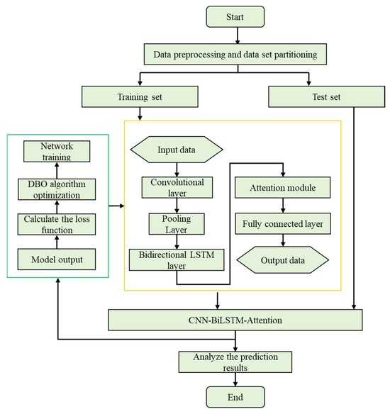
Figure 5.
Flow chart of CNN-BiLSTM-Attention optimized by DBO.
The BiLSTM hidden layer is designed to model the inherent dynamic patterns of the local features extracted by the CNN. Through iterative processing, it derives more intricate global features from these local counterparts. Subsequently, the features produced by the BiLSTM hidden layer serve as inputs to the Attention mechanism. This mechanism automatically differentiates the significance of the information extracted by the BiLSTM hidden layer, emphasizing crucial information in a weighted manner. This approach not only leverages the sequential nature of the data more effectively, but also delves into deep-level correlations. Simultaneously, the Attention mechanism mitigates the loss of historical information and accentuates key informational points, thereby minimizing the influence of redundant data on prediction outcomes.
In the next phase, the output from the Attention layer is fed into the fully connected layer, which ultimately generates the final prediction results. To enhance the model’s performance, we utilize the DBO optimization algorithm to fine-tune the model’s hyperparameters. This iterative process continually refines the prediction model, making its structure more rational and boosting its predictive accuracy. Lastly, the trained CNN-BiLSTM-Attention model is saved, and its efficacy is rigorously validated using the designated test set.
3.6. Evaluation Criteria
The models are evaluated using MAPE, RMSE, and MAE, where MAPE reflects the goodness of fit of the model, and RMSE and MAE reflect the accuracy of predictions. The smaller the values of these three metrics, the better the predictive performance of the model. The formulas corresponding to these three evaluation metrics are as follows:
Here, and represent predicted and actual values, respectively, and m denotes the number of data samples.
4. Model Training and Prediction Results Discussion
4.1. Parameter Selection and Data Preprocessing
In this study, seven crucial parameters during the cantilever casting construction process were selected as the feature values for model training These parameters mainly include the input cantilever length (L), concrete modulus of elasticity (E), segment length (l), concrete unit weight (γ), secondary dead load (P), bridge deck width (W), and bridge bottom width (w). The output prediction target is the pre-camber (y). The model establishes the physical relationship between the parameters and pre-camber through the multi-level feature fusion mechanism. The CNN convolution layer automatically identifies the geometric parameters of the cross-section geometric feature space, the BiLSTM captures the time-varying mechanical effect, and the Attention mechanism dynamically identifies the main control factors in the construction stage. The control elements of different stages of construction are revealed, and the change in the pre-camber is predicted by segment pouring. This paper collected a total of 554 sets of pre-camber data during the bridge construction phase [37,38,39,40,41]. Due to space limitations, Table 1 only lists the data for the Zhuisanhe Bridge and Ningyongjiang Extra-large Bridge.

Table 1.
Bridge parameters and characteristic values.
Before training the model, the data underwent the four following preprocessing steps:
- (1)
- Shuffle the dataset: Shuffling the dataset helps the model better learn the statistical properties of the data, preventing the model from overly depending on specific data sequences and thereby improving its generalization ability.
- (2)
- Extract features and target values: Separating the features and target values in the dataset helps the model better understand the relationship between inputs and outputs, thus making more accurate predictions.
- (3)
- Split into training and testing sets: Splitting the data into training and testing sets in a 9:1 ratio allows evaluation of the model’s performance on unseen data. The training set is used to train the model, while the testing set is used to evaluate the model’s generalization ability.
- (4)
- Normalize features and target values: Normalizing the data scales the values to a similar range, which helps accelerate model convergence and improve its stability.
4.2. DBO Algorithm Optimizes CNN-BiLSTM-Attention
When constructing and optimizing the pre-camber prediction model based on CNN-BiLSTM-Attention, the selection of hyperparameters is crucial for the model’s performance. Especially in the BiLSTM model, there are multiple hyperparameters that need careful adjustment to achieve optimal performance. Although some hyperparameters such as the number of output layer units and input data dimensions and the number of fully connected units and output dimensions have direct corresponding relationships, other key parameters such as the number of neurons, initial learning rate, and learning rate decay factor cannot be directly determined and require optimization through experimentation and algorithms. The selection of these hyperparameters not only affects the training speed and convergence of the model, but also directly relates to the accuracy of the pre-camber prediction by the model. Among these, the number of neurons, initial learning rate, and learning rate decay factor have a significant impact on pre-camber prediction. Determining the optimal size of hyperparameters through the DBO algorithm can avoid repetitive experiments and improve the accuracy of pre-camber prediction. The dung beetle population was set to 30, of which six were ball-rolling dung beetles, six were brood ball dung beetles, seven were small dung beetles, and 11 were thief dung beetles. Table 2 shows the BiLSTM hyperparameters optimized using DBO.
Table 2.
Optimal values of BiLSTM hyperparameters.
In order to verify the superiority of the algorithm used in this paper, this paper chooses to compare DBO with GWO and PSO, as shown in Table 3. The results show that the DBO algorithm is superior to GWO and PSO, and can better predict the pre-camber.
Table 3.
Comparison of algorithm prediction error.
4.3. Discussion of Prediction Results
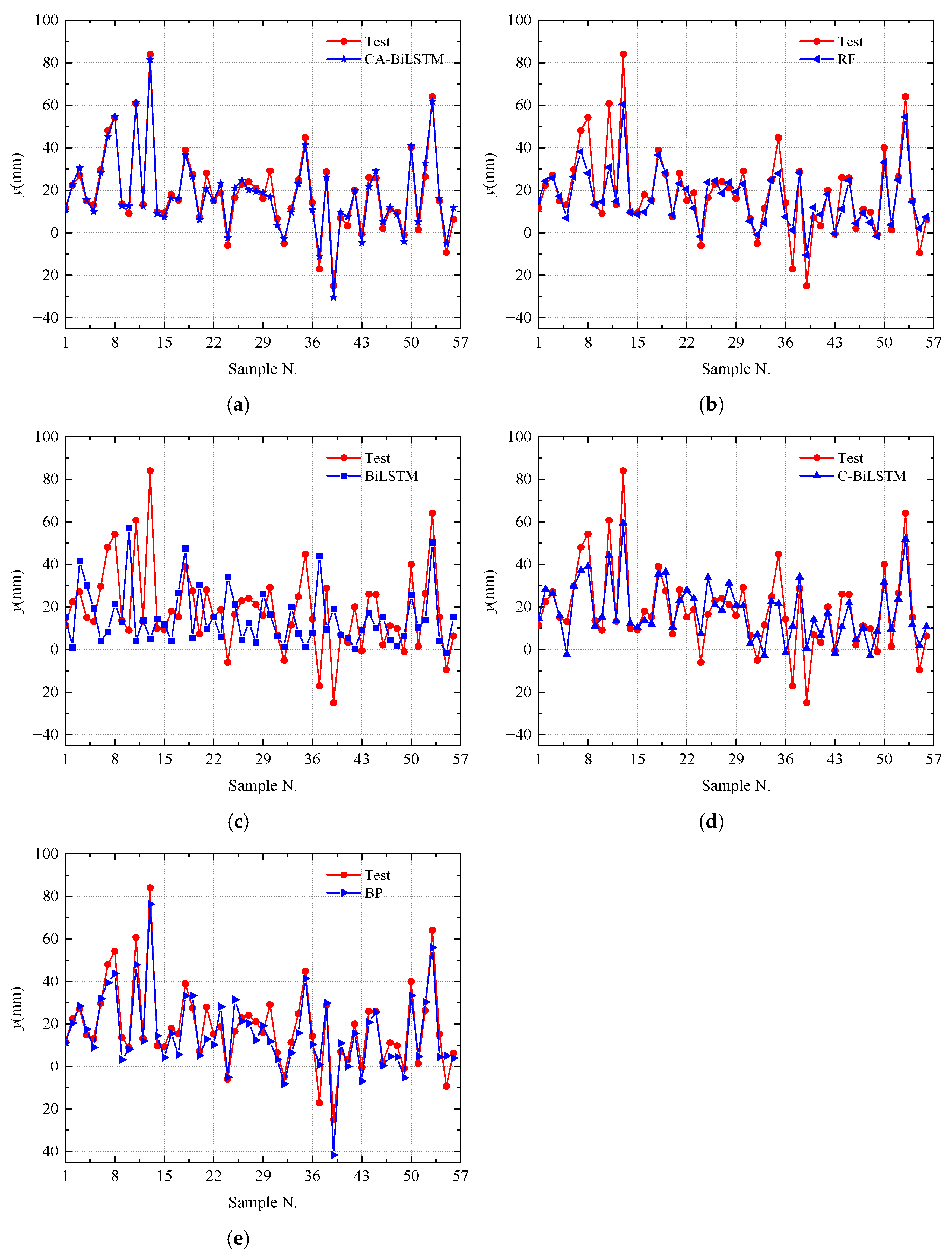
To validate the superiority of the CNN-BiLSTM-Attention model for predicting pre-camber in cantilever construction, a comparative analysis was conducted with several mainstream prediction algorithms. Figure 6 shows the prediction results of BP [42], Random Forest (RF) [43], BiLSTM, CNN-BiLSTM, and CNN-BiLSTM-Attention models. From Figure 6, it can be observed that although BiLSTM and CNN-BiLSTM can reflect the overall trend of pre-camber changes, their prediction performance is poor. The BP algorithm and Random Forest algorithm have a relatively high prediction accuracy, but they exhibit significant deviations in predicting individual data values. Compared with these algorithms, the proposed CNN-BiLSTM-Attention model in this paper achieves more accurate prediction results. Overall comparison indicates that the CNN-BiLSTM-Attention model proposed in this paper can effectively predict the trend of the pre-camber, accurately capture its changing pattern, and assess the impact of feature parameters on pre-camber accurately.
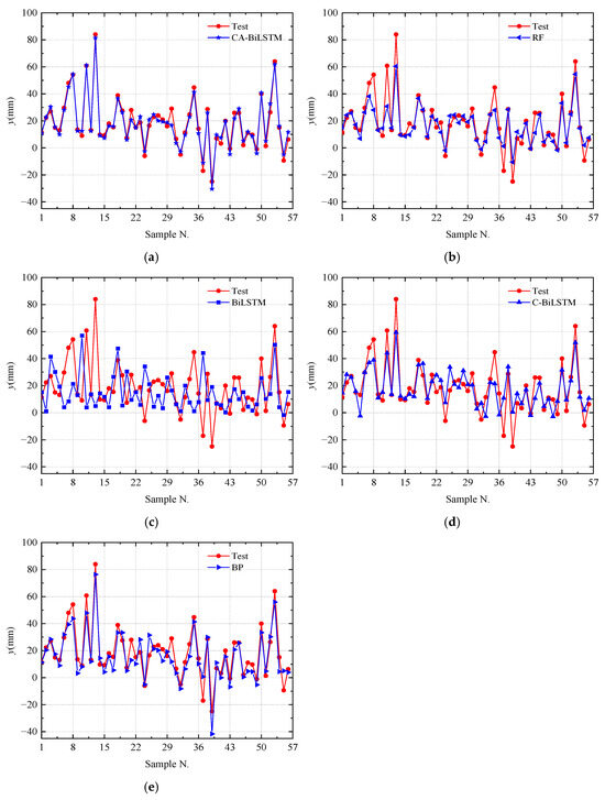
Figure 6.
Pre-camber prediction results. (a) CA-BiLSTM prediction results. (b) RF prediction results. (c) BiLSTM prediction results. (d) C-BiLSTM prediction results. (e) BP prediction results.
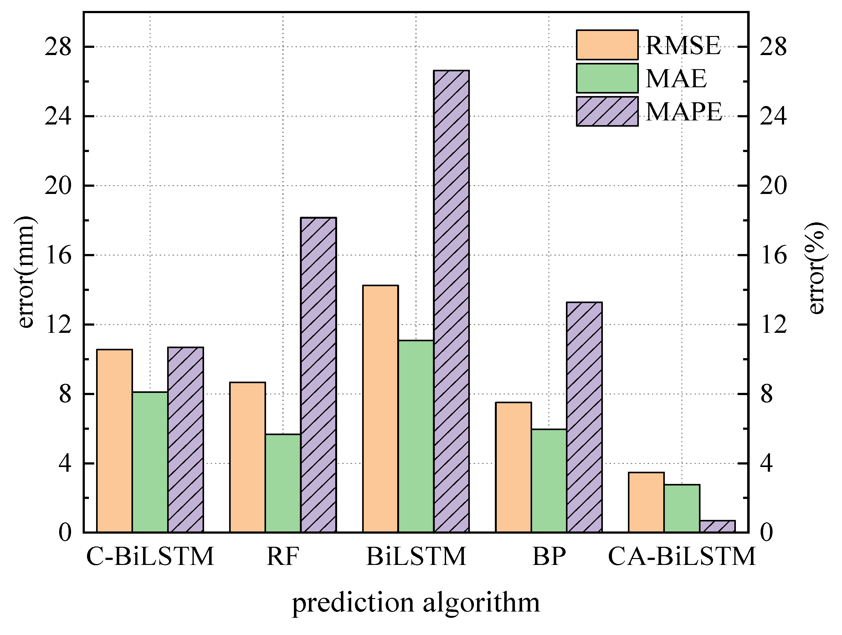
The evaluation metrics for the prediction outcomes of various models are presented in Figure 7 and Table 4. Table 4 shows that the RMSE of the BiLSTM, CNN-BiLSTM, Random Forest, and BP prediction models are ranked from highest to lowest as 14.24 mm, 10.56 mm, 8.66 mm, and 7.50 mm, respectively. The RMSE of the proposed model in this paper is 3.47 mm, which is lower than the RMSE of the other four prediction models. Regarding MAPE and MAE, the proposed model in this paper has the lowest prediction errors. In Figure 7, RMSE and MAE correspond to the numerical values on the left axis, while MAPE corresponds to the right axis values. Overall, the proposed CNN-BiLSTM-Attention prediction model in this paper outperforms the Random Forest, BP, BiLSTM, and CNN-BiLSTM models in terms of MAPE, RMSE, and MAE evaluation metrics, demonstrating significant advantages in predicting pre-camber in construction processes.
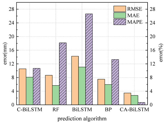
Figure 7.
Comparison of evaluation values of different models.
Table 4.
Comparison model prediction errors.
As shown in Table 3, in the predicted pre-camber results, the RMSE of the CNN-BiLSTM-Attention model is 3.47 mm, which is reduced by 10.77 mm and 7.10 mm compared to the BiLSTM and CNN-BiLSTM models, respectively. The MAE of the CNN-BiLSTM-Attention model is 2.76 mm, which is decreased by 8.32 mm and 5.34 mm compared to the BiLSTM and CNN-BiLSTM models, respectively. The MAPE index of the CNN-BiLSTM-Attention model is reduced by 25.94% and 9.99% compared to the BiLSTM and CNN-BiLSTM models, respectively. The comparative results indicate a significant improvement in the prediction accuracy of the proposed model. The model effectively combines the strengths of CNN and BiLSTM methods. Specifically, leveraging CNN’s powerful feature extraction capability enables the capture of both local and global correlations in the data, while BiLSTM excels in handling sequential data, capturing long-term dependency relationships in time-series information. Additionally, the model utilizes an attention mechanism to address the challenge of preserving key information in BiLSTM input sequences that are relatively long. It assigns varying weights to different parts of the input, ensuring crucial information receives adequate attention and effectively enhances prediction accuracy.
5. Application of CNN-BiLSTM-Attention Neural Network Model on Cantilever Casting Continuous Girder Bridge
5.1. Bridge Description
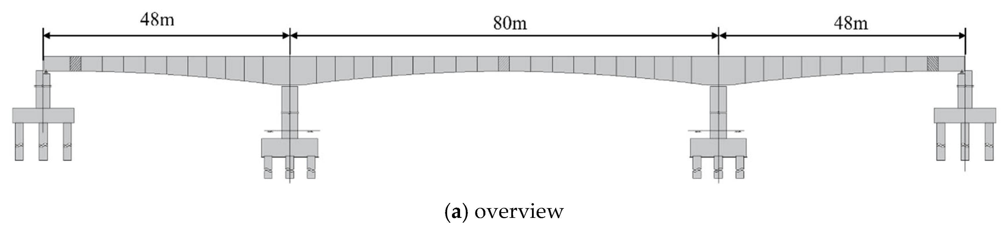
The bridge used in this study (as shown in Figure 8a) is located in Liaoning Province, China. It is a prestressed concrete continuous girder bridge with a total length of 176 m and a span configuration of (48 + 80 + 48) meters. It adopts a single-box single-chamber variable cross-section form, top girder width of 10.4 m, bottom girder width of 5.6 m, and a flange length of 2.4 m. The bottom plate varies according to a parabolic curve, with the top section height of the main pier being 4.8 m, and the section height of the mid-span and side-span being 2.5 m. Due to the presence of an existing bridge over the upstream river and to meet the span requirements without affecting normal traffic under the bridge, a balanced cantilever casting method using a hanging basket was adopted for construction (as shown in Figure 8b). The maximum cantilever girder consists of nine segments, with segments 1–4 being 3.5 m long, segments 5–9 being 4 m long, the side-span cast-in-place segment being 7.0 m long, and the closure segment being 2 m long (as shown in Figure 8c).
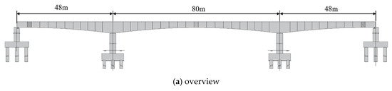
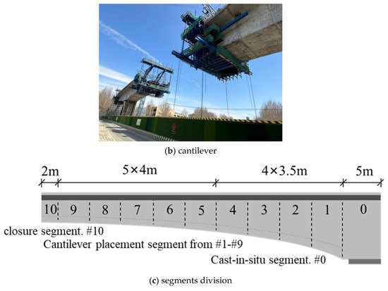
Figure 8.
Description of the continuous girder bridge: (a) overview; (b) cantilever construction; and (c) segments division.
5.2. Application of Prediction Model
The CNN-BiLSTM-Attention model established has been successfully applied to predict the pre-camber of on-site continuous girder bridges. Using the CNN-BiLSTM-Attention model, on-site experimental parameters for pre-camber prediction are input and compared with on-site monitoring results, as shown in Figure 9. In Figure 9, the left coordinate axis represents pre-camber values, corresponding to the bar chart, indicating the comparison between predicted values and on-site measured pre-camber; the right coordinate axis represents pre-camber error values, corresponding to the line graph, indicating the error values of the pre-camber for each section. Here, B denotes the edge span side of the continuous girder bridge, and Z denotes the mid-span side of the continuous girder bridge.
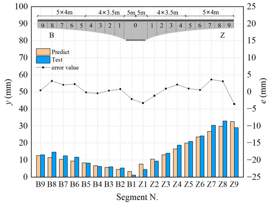
Figure 9.
Comparison of prediction of pre-camber of cantilever girder.
From Figure 9, it can be seen that the predicted values of the CNN-BiLSTM-Attention model are consistent with the actual measured pre-camber values of most cantilever sections on site. The evaluation metrics RMSE, MAE, and MAPE are 2.10 mm, 1.73 mm, and 0.23%, respectively. The maximum difference between field test values and predicted values is 3.57 mm, which meets the specification requirements. Considering the complex construction environment of bridges and the efficiency of neural networks, this level of accuracy is acceptable for deflection control. The CNN-BiLSTM-Attention model based on DBO optimization proposed in this paper can provide a reliable basis for predicting pre-camber in cantilever casting construction and ensuring the stable operation of bridges in the later stages.
6. Conclusions
In response to the prediction problem of pre-camber during the cantilever pouring process of continuous girder bridges, this paper proposes a CNN-BiLSTM-Attention model and constructs a DBO algorithm for optimizing the hyperparameters of the model. The main conclusions of this study are as follows:
- (1)
- This paper integrates an attention mechanism and combines CNN and BiLSTM networks to propose a CNN-BiLSTM-Attention prediction model optimized by the DBO algorithm. The model utilizes seven parameter, including the cantilever length, concrete unit weight, and concrete elastic modulus as input features, comprehensively taking into account various factors that affect bridge pre-camber.
- (2)
- Compared with four other prediction algorithms, the CNN-BiLSTM-Attention model proposed in this paper performs the best on the pre-camber dataset. Specifically, the model achieves an MAE (Mean Absolute Error) of 2.76 mm, RMSE (Root Mean Square Error) of 3.47 mm, and MAPE (Mean Absolute Percentage Error) of 0.70%. In terms of the MAE, RMSE, and MAPE, for these three evaluation metrics, the model outperforms the other four models, demonstrating higher prediction accuracy and stronger generalization ability.
- (3)
- Applying the trained model to predict the pre-camber of the girder section under construction results in small errors between predicted and actual values. The model demonstrates high prediction accuracy, with RMSE, MAE, and MAPE values of 2.10 mm, 1.73 mm, and 0.23%, respectively. This model exhibits strong applicability for complex engineering systems, providing new insights for intelligent control in bridge construction.
Future Research: The DBO-CNN-BiLSTM-Attention model proposed in this paper provides an efficient prediction tool for the pre-camber of cantilever casting construction of continuous girder bridges. However, the model still has limitations such as insufficient embedding of physical mechanisms. Future research will increase the eigenvalues of environmental conditions (such as temperature, humidity, etc.), focus on the development of hybrid modeling methods embedded in physical information, establish a cross-bridge transfer learning framework, and achieve real-time predictive control of the construction process through edge computing deployment, and ultimately promote the leap-forward development of pre-camber prediction from offline analysis to online decision making.
Author Contributions
Conceptualization, H.L. and X.G.; methodology, H.L.; validation, M.L.; formal analysis, J.Z.; investigation, M.L.; data curation, Z.C.; writing—original draft preparation, J.Z.; writing—review and editing, J.Z.; visualization, J.Z.; supervision, X.G. All authors have read and agreed to the published version of the manuscript.
Funding
This study was supported by discipline innovation team of Liaoning Technical University (grant number LNTU20TD-12) and additional support was funded by Liaoning Province Key R&D Plan Project (No. 2018230008).
Data Availability Statement
All data supporting the findings in this study are available from the corresponding author upon reasonable request.
Acknowledgments
We thank Liaoning Technical University, China for providing the funding and facilities to carry out the experimental work presented in this study.
Conflicts of Interest
Authors Xiangen Gong, Ming Lei and Zimu Chen were employed by the company China Construction Fifth Engineering Division Corp., Ltd. The remaining authors declare that the research was conducted in the absence of any commercial or financial relationships that could be construed as a potential conflict of interest.
References
- Hu, F.; Huang, P.; Dong, F.; Blanchet, A. Stability Safety Assessment of Long-Span Continuous Girder Bridges in Cantilever Construction. J. Intell. Fuzzy Syst. 2018, 35, 4027–4035. [Google Scholar] [CrossRef]
- Ouyang, Y.; Huang, J.; Song, K. Development of Rhombus Hanging Basket Walking Track Robot for Cantilever Casting Construction in Bridges. Appl. Sci. 2023, 13, 10635. [Google Scholar] [CrossRef]
- Breccolotti, M. Eigenfrequencies of Continuous Prestressed Concrete Bridges Subjected to Prestress Losses. Structures 2020, 25, 138–146. [Google Scholar] [CrossRef]
- Pregnolato, M. Bridge Safety Is Not for Granted-A Novel Approach to Bridge Management. Eng. Struct. 2019, 196, 109193. [Google Scholar] [CrossRef]
- Yoshida, I.; Sekiya, H.; Wada, R.; Ohno, T.; Morichika, S.; Yasuda, A.; Yoshiura, N. Preliminary Field Estimation of Vertical Displacements of Prestressed Concrete Bridges under Construction Based on Measured Strains and Inclinations. Structures 2024, 65, 106651. [Google Scholar] [CrossRef]
- Jeon, J.-C.; Lee, H.-H. Development of Displacement Estimation Method of Girder Bridges Using Measured Strain Signal Induced by Vehicular Loads. Eng. Struct. 2019, 186, 203–215. [Google Scholar] [CrossRef]
- Chen, F.; Liu, X.; Zhang, H.; Luo, Y.; Lu, N.; Liu, Y.; Xiao, X. Assessment of Fatigue Crack Propagation and Lifetime of Double-Sided U-Rib Welds Considering Welding Residual Stress Relaxation. Ocean Eng. 2025, 332, 121400. [Google Scholar] [CrossRef]
- Zhang, H.; Liu, H.; Deng, Y.; Cao, Y.; He, Y.; Liu, Y.; Deng, Y. Fatigue Behavior of High-Strength Steel Wires Considering Coupled Effect of Multiple Corrosion-Pitting. Corros. Sci. 2025, 244, 112633. [Google Scholar] [CrossRef]
- Zhang, H.; Liu, H.; Kuai, H. Stress Intensity Factor Analysis for Multiple Cracks in Orthotropic Steel Decks Rib-to-Floorbeam Weld Details under Vehicles Loading. Eng. Fail. Anal. 2024, 164, 108705. [Google Scholar] [CrossRef]
- Mante, D.M.; Barnes, R.W.; Isbiliroglu, L.; Hofrichter, A.; Schindler, A.K. Effective Strategies for Improving Camber Predictions in Precast, Prestressed Concrete Bridge Girders. Transp. Res. Rec. J. Transp. Res. Board 2019, 2673, 342–354. [Google Scholar] [CrossRef]
- Robertson, I.N. Prediction of Vertical Deflections for a Long-Span Prestressed Concrete Bridge Structure. Eng. Struct. 2005, 27, 1820–1827. [Google Scholar] [CrossRef]
- Yao, S.; Peng, B.; Wang, L.; Chen, H. Estimation Formula of Finished Bridge Pre-Camber in Continuous Rigid-Frame Bridges. Sci. Rep. 2022, 12, 16034. [Google Scholar] [CrossRef]
- Zhang, Y.B.; Liu, D.P. Research on Setting of Pre-Camber of Long-Span Continuous Rigid Frame Bridge with High Piers. Adv. Mater. Res. 2011, 255–260, 821–825. [Google Scholar] [CrossRef]
- Tian, Y.; Zhang, J.; Xia, Q.; Li, P. Flexibility Identification and Deflection Prediction of a Three-Span Concrete Box Girder Bridge Using Impacting Test Data. Eng. Struct. 2017, 146, 158–169. [Google Scholar] [CrossRef]
- Deng, Y.; Ju, H.; Zhong, G.; Li, A. Data Quality Evaluation for Bridge Structural Health Monitoring Based on Deep Learning and Frequency-Domain Information. Struct. Health Monit. 2023, 22, 2925–2947. [Google Scholar] [CrossRef]
- Ju, H.; Shi, H.; Shen, W.; Deng, Y. An Accurate and Low-Cost Vehicle-Induced Deflection Prediction Framework for Long-Span Bridges Using Deep Learning and Monitoring Data. Eng. Struct. 2024, 310, 118094. [Google Scholar] [CrossRef]
- Zhao, H.; Ding, Y.; Li, A.; Ren, Z.; Yang, K. Live-Load Strain Evaluation of the Prestressed Concrete Box-Girder Bridge Using Deep Learning and Clustering. Struct. Health Monit. 2020, 19, 1051–1063. [Google Scholar] [CrossRef]
- Xayasouk, T.; Lee, H.; Lee, G. Air Pollution Prediction Using Long Short-Term Memory (LSTM) and Deep Autoencoder (DAE) Models. Sustainability 2020, 12, 2570. [Google Scholar] [CrossRef]
- Liu, D.-R.; Hsu, Y.-K.; Chen, H.-Y.; Jau, H.-J. Air Pollution Prediction Based on Factory-Aware Attentional LSTM Neural Network. Computing 2021, 103, 75–98. [Google Scholar] [CrossRef]
- Fong, I.H.; Li, T.; Fong, S.; Wong, R.K.; Tallón-Ballesteros, A.J. Predicting Concentration Levels of Air Pollutants by Transfer Learning and Recurrent Neural Network. Knowl.-Based Syst. 2020, 192, 105622. [Google Scholar] [CrossRef]
- Abubakr, M.; Rady, M.; Badran, K.; Mahfouz, S.Y. Application of Deep Learning in Damage Classification of Reinforced Concrete Bridges. Ain Shams Eng. J. 2024, 15, 102297. [Google Scholar] [CrossRef]
- Moon, H.S.; Hwang, Y.K.; Kim, M.K.; Kang, H.-T.; Lim, Y.M. Application of Artificial Neural Network to Predict Dynamic Displacements from Measured Strains for a Highway Bridge under Traffic Loads. J. Civ. Struct. Health Monit. 2022, 12, 117–126. [Google Scholar] [CrossRef]
- Marasco, G.; Oldani, F.; Chiaia, B.; Ventura, G.; Dominici, F.; Rossi, C.; Iacobini, F.; Vecchi, A. Machine Learning Approach to the Safety Assessment of a Prestressed Concrete Railway Bridge. Struct. Infrastruct. Eng. 2022, 20, 566–580. [Google Scholar] [CrossRef]
- Shan, J.; Zhang, X.; Liu, Y.; Zhang, C.; Zhou, J. Deformation Prediction of Large-Scale Civil Structures Using Spatiotemporal Clustering and Empirical Mode Decomposition-Based Long Short-Term Memory Network. Autom. Constr. 2024, 158, 105222. [Google Scholar] [CrossRef]
- Xu, Z.; Chen, J.; Shen, J.; Xiang, M. Recursive Long Short-Term Memory Network for Predicting Nonlinear Structural Seismic Response. Eng. Struct. 2022, 250, 113406. [Google Scholar] [CrossRef]
- Li, X.; Zhang, W.; Ding, Q. Deep Learning-Based Remaining Useful Life Estimation of Bearings Using Multi-Scale Feature Extraction. Reliab. Eng. Syst. Saf. 2019, 182, 208–218. [Google Scholar] [CrossRef]
- Hu, K.; Wu, X. Mode Shape Prediction Based on Convolutional Neural Network and Autoencoder. Structures 2022, 40, 127–137. [Google Scholar] [CrossRef]
- Elmaz, F.; Eyckerman, R.; Casteels, W.; Latré, S.; Hellinckx, P. CNN-LSTM Architecture for Predictive Indoor Temperature Modeling. Build. Environ. 2021, 206, 108327. [Google Scholar] [CrossRef]
- Wang, X.; Bai, Y.; Liu, X. Prediction of Railroad Track Geometry Change Using a Hybrid CNN-LSTM Spatial-Temporal Model. Adv. Eng. Inform. 2023, 58, 102235. [Google Scholar] [CrossRef]
- Méndez, M.; Merayo, M.G.; Núñez, M. Long-Term Traffic Flow Forecasting Using a Hybrid CNN-BiLSTM Model. Eng. Appl. Artif. Intell. 2023, 121, 106041. [Google Scholar] [CrossRef]
- Feng, H.; Huang, S.; Zhou, D.-X. Generalization Analysis of CNNs for Classification on Spheres. IEEE Trans. Neural Netw. Learn. Syst. 2023, 34, 6200–6213. [Google Scholar] [CrossRef] [PubMed]
- Sayeed, A.; Choi, Y.; Eslami, E.; Lops, Y.; Roy, A.; Jung, J. Using a Deep Convolutional Neural Network to Predict 2017 Ozone Concentrations, 24 Hours in Advance. Neural Netw. 2020, 121, 396–408. [Google Scholar] [CrossRef] [PubMed]
- Jin, Y.; Lee, S.M. Sampled-Data State Estimation for LSTM. IEEE Trans. Neural Netw. Learn. Syst. 2025, 36, 2300–2313. [Google Scholar] [CrossRef] [PubMed]
- Suebsombut, P.; Sekhari, A.; Sureephong, P.; Belhi, A.; Bouras, A. Field Data Forecasting Using LSTM and Bi-LSTM Approaches. Appl. Sci. 2021, 11, 11820. [Google Scholar] [CrossRef]
- Fang, P.; Zhou, J.; Roy, S.K.; Ji, P.; Petersson, L.; Harandi, M.T. Attention in Attention Networks for Person Retrieval. IEEE Trans. Pattern Anal. Mach. Intell. 2021, 44, 4626–4641. [Google Scholar] [CrossRef]
- Xue, J.; Shen, B. Dung Beetle Optimizer: A New Meta-Heuristic Algorithm for Global Optimization. J. Supercomput. 2023, 79, 7305–7336. [Google Scholar] [CrossRef]
- Wang, X. Study on Technology of (72+128+72) m Prestressed Concrete Continuous Beam Bridge Construction Control; Shijiazhuang Tiedao University: Shijiazhuang, China, 2020. [Google Scholar]
- Li, P. Deformation Prediction Method for Cantilever Construction of Long-Span Continuous Rigid Frame Bridge; Beijing Jiaotong University: Beijing, China, 2021. [Google Scholar]
- Xiao, J. Research on Cantilever Construction Control and Temperature Effects of Long Span PC Continuous Beam Bridge; Southwest Jiaotong University: Chengdu, China, 2018. [Google Scholar]
- Chen, Y. Study on Cantilever Casting Technology for Geometric and Mechanical Performance of The Long-Span Prestressed Concrete Continuous Rigid Frame Bridge; Southeast University: Nanjing, China, 2018. [Google Scholar]
- Zhang, Y. Study on the Construction Control of Large-Span Prestressed Continuous Girder Bridge; Hefei University of Technology: Hefei, China, 2023. [Google Scholar]
- Chen, D.S.; Jain, R.C. A Robust Backpropagation Learning Algorithm for Function Approximation. IEEE Trans. Neural Netw. 1994, 5, 467–479. [Google Scholar] [CrossRef]
- Han, S.; Kim, H.; Lee, Y.-S. Double Random Forest. Mach. Learn. 2020, 109, 1569–1586. [Google Scholar] [CrossRef]


Disclaimer/Publisher’s Note: The statements, opinions and data contained in all publications are solely those of the individual author(s) and contributor(s) and not of MDPI and/or the editor(s). MDPI and/or the editor(s) disclaim responsibility for any injury to people or property resulting from any ideas, methods, instructions or products referred to in the content. |
© 2025 by the authors. Licensee MDPI, Basel, Switzerland. This article is an open access article distributed under the terms and conditions of the Creative Commons Attribution (CC BY) license (https://creativecommons.org/licenses/by/4.0/).