A Numerical Investigation of the Relationship Between Air Quality, Topography, and Building Height in Populated Hills

Abstract

Urban population growth has led to increased air pollution, influenced by disrupted wind patterns and the heterogeneous distribution of pollutants. Although the relationship between urban form and air quality is well recognized, it is often examined in isolation and through simplified urban geometries. This study addresses these limitations by numerically analyzing pollutant dispersion in densely populated hillside areas using idealized but topographically representative building geometries. A three-dimensional microclimatic simulation is conducted with ENVI-met software, incorporating parametric slope angles and building height variations. The results demonstrate that both slope steepness and building height significantly affect local pollutant concentrations: steeper slopes and taller buildings are associated with higher peak pollution values in the environment. Additionally, the simulation results show that vegetation is critical in mitigating pollution, acting as a natural barrier that enhances dispersion. These findings highlight the need for slope-sensitive urban planning and strategically integrating vegetation in hillside developments to improve air quality in complex urban terrains.

1. Introduction

Since 2008, most of the global population has resided in urban areas, and this trend is expected to intensify in the coming decades. By 2030, the urban population is projected to triple compared to 2000 [1]. This rapid urbanization often leads to increased building density and significant transformations in urban form, affecting air pollutants’ dispersion and accumulation [2,3]. Compact urban configurations, especially those characterized by narrow street canyons and limited ventilation, tend to trap pollutants and degrade air quality at the pedestrian level [4].

Despite the clear relationship between urban planning and air quality, these fields are frequently addressed in isolation, limiting the potential for integrated solutions to urban environmental health challenges [5]. In recent years, research has increasingly focused on understanding how specific urban patterns—such as building geometry, street layout, land use, and vegetation—affect pollutant dispersion and exposure at the microscale. A common approach to exploring these relationships involves using computational fluid dynamics (CFD) models, which are considered reliable and accessible tools for simulating airflow and pollutant transport in urban environments [4].

However, a critical limitation in many CFD-based studies is their reliance on idealized or overly simplified representations of urban geometry. Common modeling approaches often use repetitive building blocks, uniform heights, and flat terrain to reduce computational complexity, overlooking the diverse and irregular forms in real urban environments [6]. These simplifications can significantly affect simulation results’ accuracy, realism, and applicability, as CFD outcomes are susceptible to geometric detail, boundary conditions, and physical assumptions [7,8,9]. Geometry, in particular, has been widely recognized as one of the key determinants of pollutant behavior at the pedestrian scale [10].

Another variable frequently considered in urban air quality studies is vegetation. Green infrastructure is often promoted as a nature-based solution to improve air quality, yet its impact depends heavily on local wind regimes, temperature gradients, and urban morphology. In some scenarios, vegetation may hinder ventilation and increase pollutant concentrations in low-flow areas [2]. Notably, many studies investigating the role of vegetation assume a flat terrain, ignoring how slope and elevation influence airflow and pollutant dynamics.

This simplification poses a significant limitation when studying urban areas in topographically complex regions, such as informal settlements built on hillsides. In Latin America, for instance, neighborhoods like the favelas of Rio de Janeiro and the Barrios Altos of Lima often feature steep terrain and irregular constructions. These physical characteristics can generate localized meteorological phenomena, such as anabatic and katabatic winds, gravity currents, and atmospheric hydraulic jumps, strongly influencing pollutant dispersion [11]. Ignoring these effects reduces the reliability of simulation results and limits their usefulness for urban planning in such contexts.

Moreover, the interaction between topography and air quality is also intertwined with social inequality. Numerous studies from diverse contexts—including the United Kingdom, China, Canada, South Africa, and Colombia—have documented a disproportionate concentration of atmospheric pollution in lower-income neighborhoods [12]. These areas also tend to have less green infrastructure—up to 21% less than wealthier neighborhoods—reducing their capacity to mitigate pollution impacts [13,14]. These patterns reflect a broader environmental justice issue that remains insufficiently addressed in modeling studies, particularly in the Global South.

Although prior research has explored how vegetation, urban form, and pollution interact, most studies do so under simplified assumptions. Few studies have examined how building geometry, vegetation, pollutant sources, and terrain slope interact simultaneously to influence air quality in realistic urban settings. Despite its relevance in many urban areas, the omission of terrain slope represents a notable research gap.

This study aims to fill that gap by investigating how these four variables—vegetation, pollutant concentration, building geometry, and terrain slope—interact to shape air quality in complex urban environments. Using ENVI-met, a validated micro-meteorological model commonly employed in urban studies [15,16], we conduct a numerical sensitivity analysis to assess each variable’s individual and combined effects. While previous work has utilized ENVI-met to explore air quality, this study offers the following two key contributions: (1) the incorporation of terrain slope as a variable, addressing a significant limitation in earlier studies that typically assumed flat surfaces, and (2) the simulation of multiple pollutants, including a user-defined scalar, to gain a more nuanced understanding of pollutant behavior under varied urban configurations.

By integrating detailed geometry, vegetation, emission sources, and topography in the modeling framework, this study contributes a novel perspective on the spatial dynamics of air pollution in urban settings. The findings are particularly relevant for cities in low- and middle-income regions, where informal urbanization, socioeconomic vulnerability, and complex terrain frequently coincide, posing challenges to environmental justice and sustainable urban design.

The following section presents the methodological approach used for the simulations, including model configuration, variable selection, and simulation design.

2. Methodology

This study employs ENVI-met 5.1, a validated 3D microclimatic CFD model, to investigate how topography, building height, and vegetation influence pollutant dispersion in idealized hillside urban environments. The methodological approach consists of four main steps. First, average meteorological conditions (e.g., temperature, wind speed, and wind direction) and representative topographic profiles are derived from real-world data from hillside districts in Lima, Peru. Second, using these inputs, a base model geometry is created, incorporating simplified yet representative urban layouts and environmental conditions. Third, a parametric analysis is conducted by systematically varying terrain slopes, building heights, and vegetation configurations to isolate their effects on pollutant concentration and distribution patterns. Finally, trends are identified by comparing simulation results across different scenarios. The ENVI-met model solves the Reynolds-Averaged Navier–Stokes equations with turbulence closure schemes, allowing for high-resolution wind flow, heat transfer, and pollutant transport simulations in complex urban terrains.

2.1. Model Description

ENVI-met is a non-hydrostatic 3D CFD model that solves the Reynolds-Averaged Navier–Stokes (RANS) equations using a turbulence closure scheme. It supports the simulation of airflow, heat transfer, humidity, and pollutant dispersion at a microscale resolution [17]. Vegetation effects are included as aerodynamic sink terms, and advection–diffusion equations govern pollutant transport. This study used version 5.1, with the chemistry module deactivated and a user-defined pollutant included via scalar emissions.

2.2. Case Study Area: Lima, Peru

Lima, the capital of Peru, is located on the central western coast of South America, bordered by the Pacific Ocean and the foothills of the Andes [18]. Its topography is highly heterogeneous, comprising flat coastal plains, river valleys, and steep hills [18]. Informal settlements have proliferated on these hillsides, particularly in districts such as San Juan de Lurigancho and Villa María del Triunfo, where slopes frequently exceed 20%, creating substantial challenges for infrastructure provision and environmental management [19].

Lima’s climate is classified as subtropical desert (BWh) according to the Köppen classification [20]. Despite this, the city experiences persistent humidity and cloud cover, especially during the austral winter (June–September), due to the cooling influence of the Humboldt Current. Annual precipitation averages below 15 mm, and winter temperatures typically range between 16 °C and 18 °C [21].

Rapid urban growth has resulted in an uneven distribution of green spaces and intensified air quality concerns. Municipal initiatives such as the Lima Ecological Infrastructure Strategy (LEIS) aim to enhance urban resilience through integrated landscape and water management [22].

Local vegetation includes drought-resistant species commonly used in urban forestry and reforestation programs, such as Algarrobo (Prosopis pallida), Cedar (Cedrela spp.), Tara (Caesalpinia spinosa), Huarango (Prosopis nigra), and Molle serrano (Schinus molle) [13,23]. These species are valued for their adaptability and contribution to urban ecological restoration.

Given its complex topography, semi-arid climate, and prevalence of informal hillside development, Lima provides a highly relevant context to investigate the interactions among terrain, vegetation, built form, and air quality in rapidly urbanizing environments.

2.3. Simulation Design and Variable Selection

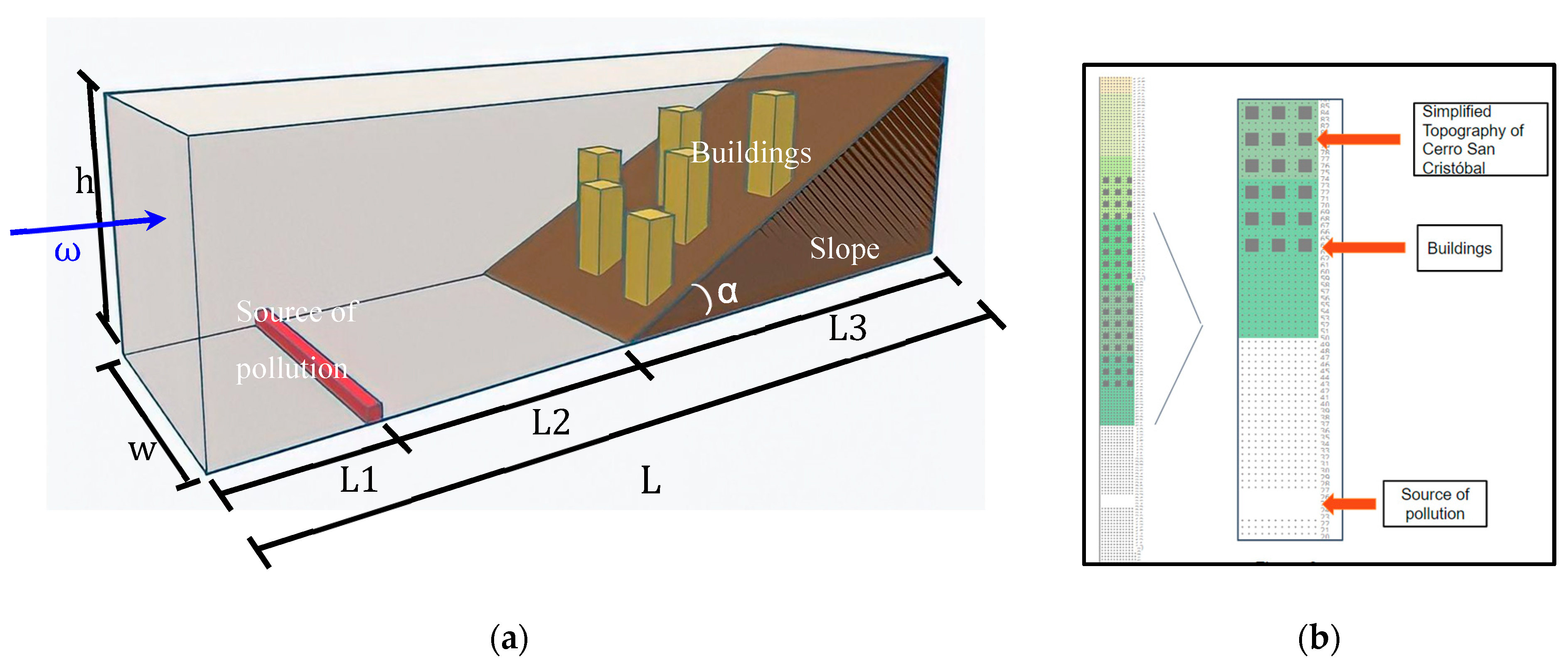
Figure 1 shows the geometric configuration used for the simulations. In part (a), a three-dimensional schematic of the idealized base case is presented, showing a domain divided into the following three main sections: a flat inlet zone where the source of contamination is located at ground level; a central section with buildings evenly distributed on a sloping terrain; and an outlet zone where the wind flow leaves the domain. The wind direction (ω) is plotted perpendicular to the slope, simulating Lima’s prevailing coastal flow conditions. Part (b) of the figure shows a top view of the same domain, modeled in the ENVI-met SPACES platform. It shows the simplified topography of a representative sector of the San Cristobal hill, as well as the spatial distribution of green areas (in green), buildings (gray blocks), and the emission source (red box at the base of the slope). In an idealized but realistic way, this configuration seeks to represent a hillside urban environment, allowing us to analyze the combined effect of slope, building height, and vegetation on the dispersion of pollutants.

The geometric configuration parameters summarized in

Table 1. Summary of the geometric configuration of the base model.

Parameter	Values	Justification
Slope	22%, 44%, 66%	Reflects typical and extreme conditions in Lima’s informal hillsides
Buildings	6 m, 9 m, 12 m	Represents common low-rise configurations in peri-urban areas
Vegetation types	None, Hedges, Trees + Hedges	Based on native species used in municipal reforestation programs
Time of day	8:00, 18:00, 20:00	Matches Lima’s daily traffic peaks and meteorological transitions, as shown in Figure 2a. These hours coincide with peak vehicle activity and elevated emission rates, making them critical moments for evaluating pollution levels
Pollutants	NO2, PM10, user-defined scalar	Reflects traffic-related emissions reported by local environmental agencies

were selected to represent a realistic but idealized urban hillslope environment typical of Lima’s populated areas. The slope value of 22% corresponds to the average inclination of many informal settlements on the hillsides of districts such as San Juan de Lurigancho and Villa María del Triunfo. The domain dimensions (L1, L2, and L3 and the lengths in the X, Y, and Z directions) were chosen to provide a sufficiently large simulation area that captures flow development, pollutant dispersion, and terrain effects while maintaining computational feasibility.

To capture the combined effects of terrain, urban form, and vegetation, we conducted a parametric analysis based on the following key variables:

This combination of parameters resulted in a total of 81 simulation runs, encompassing all possible permutations of slope, building height, vegetation type, and time of day. This full factorial design allowed for a robust comparative analysis of how each variable—and their interactions—influenced pollutant dispersion.

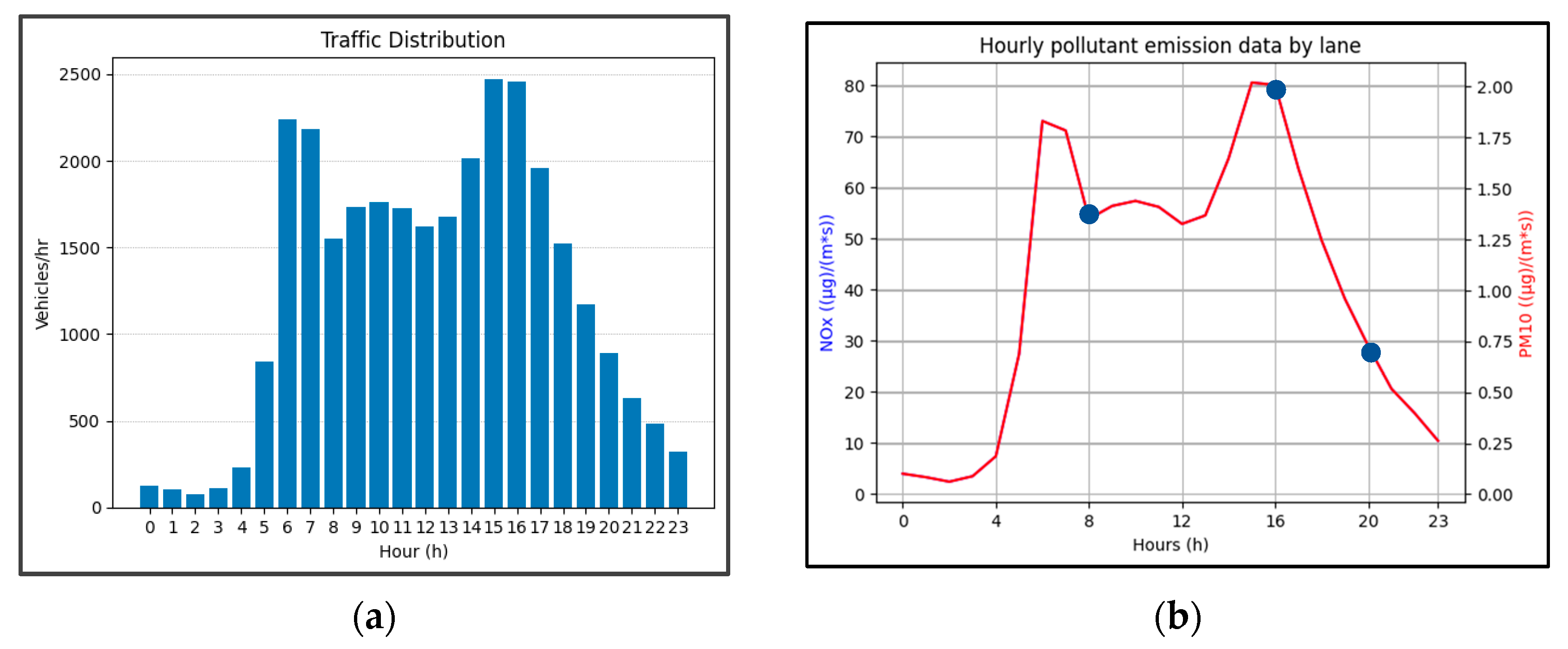
To ensure temporal realism, traffic-based emission patterns were incorporated into the model, as shown in Figure 2.

The pollutant dispersion was modeled based on a temporal traffic profile to simulate realistic urban emissions. Figure 2a shows the hourly vehicle distribution used in the simulations, which was derived from typical traffic patterns observed in urban Lima. Traffic density peaks occurred during the morning (8:00–9:00) and evening (18:00–20:00) hours, reflecting commuter activity.

Figure 2b presents the corresponding emission rates used in the ENVI-met model for the following two pollutants: NO_x (blue line) and PM₁₀ (red line). These were scaled proportionally to the vehicle count per hour and assigned to line sources in the model. The user-defined pollutant, which was also simulated, maintained a constant emission rate throughout the day for baseline comparison purposes.

2.4. Model Configurations

ENVI-met solves the Reynolds-Averaged Navier–Stokes (RANS) equations with turbulence closure and incorporates wind flow, thermal profiles, pollutant dispersion, and vegetation interactions at a high spatial resolution of 2 m.

• Domain dimensions: 456 m (length, x), 279 m (width, y), 200 m (height, z).
• Grid resolution: 2 m × 2 m × 2 m.
• Total cells: 669,600.
• Slope: constant across the domain, beginning after a 44 m flat buffer.
• Pollution source: line source simulating traffic emissions placed 44 m from the inlet.

Each simulation was run for 8 h, starting at 08:00, 18:00, or 22:00, depending on the scenario. The first hour of each simulation served as a spin-up period to allow atmospheric and surface conditions to stabilize, following ENVI-met best practices. Boundary conditions were set as open on the lateral and top edges and reflective on the ground and building surfaces.

2.5. Meteorological Input

The simulations assumed realistic local weather conditions representative of Lima, based on the SENAMHI records shown in

Table 2. Meteorological parameters.

Parameter	Value
Wind speed (m/s)	2 m/s
Wind direction (°)	180° (southerly)
Relative humidity (%)	56–95%
Temperature (°C)	15–24 °C

.

These values reflect typical wintertime conditions (June–August), critical due to atmospheric stability and frequent pollution accumulation.

2.6. Vegetation Scenarios

Vegetation configurations were selected based on local forestry guidelines and species commonly used in municipal reforestation efforts. Conceptually, species such as Algarrobo (Prosopis pallida), Tara (Caesalpinia spinosa), Huarango (Prosopis nigra), and Molle serrano (Schinus molle) were considered due to their prevalence in Lima and adaptability to arid conditions. However, for modeling purposes, vegetation was simplified into the following two structural types:

1.

Trees with characteristics equivalent to Schinus molle (height, canopy density, and LAD).

2.

Hedges with typical street-level planting density.

The following three green infrastructure scenarios were tested:

• No vegetation
• Hedges every 6 m (between buildings)
• Trees + hedges every 6 m (between buildings)

Vegetation elements were represented using Leaf Area Density (LAD) values (

Table 3. Leaf Area Density (LAD) values for vegetation elements.

Element	LAD (m2/m3)
Trees	1
Hedges	0.098

) and incorporated as aerodynamic and thermodynamic sinks in the momentum and scalar transport equations.

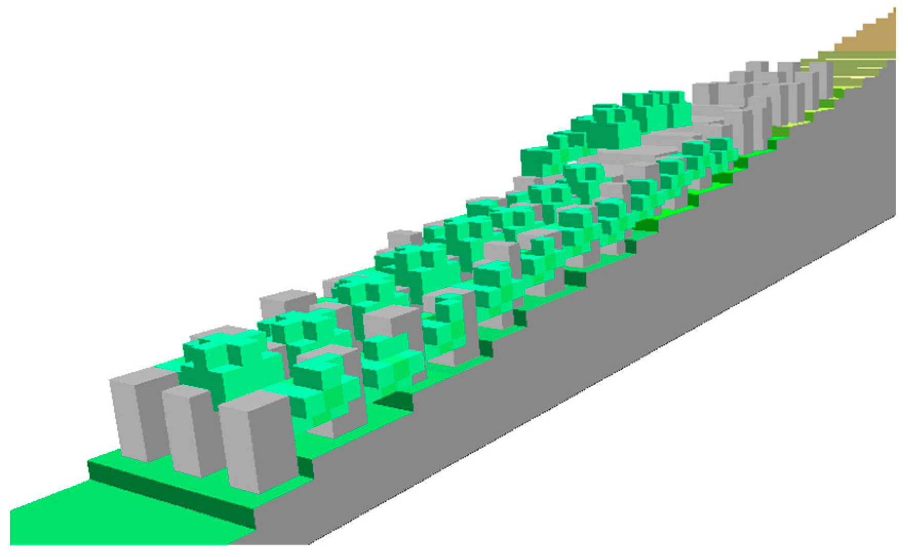
The model incorporated vegetation elements as sink terms in both the momentum and scalar transport equations, accounting for their influence on airflow, turbulence, and pollutant removal. Figure 3 illustrates the 3D simulation domain, where green blocks represent vegetation and gray blocks represent buildings. This visualization supports the spatial analysis of vegetation distribution relative to urban structures and its environmental impact.

2.7. Output Variables

The output parameters analyzed in this study included pollutant concentration (NO₂, PM₁₀, and a user-defined scalar), potential temperature—used as an indicator of atmospheric stability—and wind velocity magnitude, which reflects wind-driven dispersion capacity. In addition, the contaminated area, defined as the surface exceeding baseline concentration thresholds, was evaluated, along with pedestrian-level concentration, measured at a height of 1.5 m above ground to represent direct human exposure in urban environments.

2.8. Validation and Uncertainty of the Model

As with any simulation tool, ENVI-met introduces inherent uncertainties due to its simplified representation of real-world dynamics. While this study does not include direct validation against field data, we follow the approach of previous works, such as the residence time study and [24], who also did not validate the model within their studies, citing the extensive validation of ENVI-met in other contexts.

Given the lack of suitable measurement data for hillside urban environments, our goal is not to reproduce exact concentration values, but rather to identify robust spatial and temporal trends. This focus on comparative analysis, rather than absolute outputs, is aligned with the purpose of the model application and ensures that the findings remain valuable for informing urban planning in complex terrains.

3. Results

Of the 111 simulations conducted, this section presents results from the long-duration (8 h) runs, which are more representative of full diurnal pollutant dynamics in complex terrains. While 1 h simulations with vegetation were also performed, they are addressed separately in Section 3.4 and Section 3.5 due to their localized and short-term impacts. The results are organized by key variables—time of day, slope, building height, and vegetation—to identify individual effects and interactions on pollutant concentration, dispersion extent, and pedestrian-level exposure.

3.1. Temporal Variation in Pollutant Dispersion

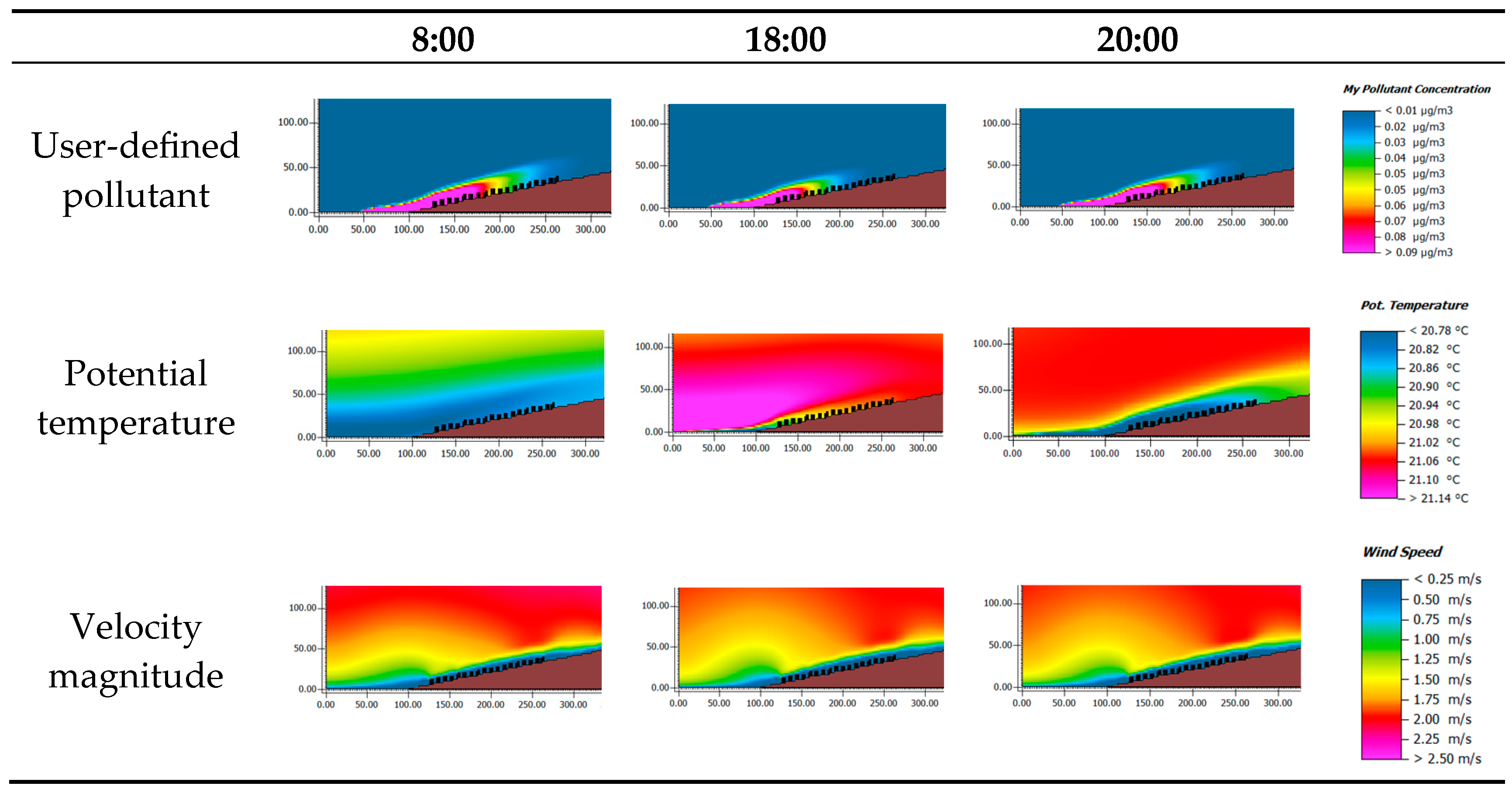
To evaluate how time of day affects air pollutant behavior, simulations were run for the following three key periods: 08:00, 18:00, and 20:00. Figure 4 illustrates how pollutant concentration, potential temperature, and wind velocity vary throughout the day in a scenario with a 22% slope and 9 m building height. These visualizations reveal the diurnal transition in atmospheric conditions and its impact on pollutant dispersion.

The results in Figure 4 show a clear diurnal progression in atmospheric dynamics and their effect on pollutant behavior.

At 08:00, pollutant concentrations are more broadly dispersed along and above the slope. The plume reaches higher elevations and greater horizontal distances. This extended dispersion is driven by stronger wind speeds, exceeding 2.25 m/s in the upper slope region, and is supported by a near-neutral thermal structure. The potential temperature profile increases gradually with height (from ~20.80 °C to ~21.05 °C), indicating limited but sufficient vertical mixing. These conditions favor horizontal advection and the gradual dilution of pollutants away from the source.

At 18:00, dispersion becomes more confined. The pollutant plume remains closer to the ground, with reduced upslope penetration. A pronounced surface inversion forms near the base of the slope, as shown by the sharp vertical gradient in potential temperature. This inhibits near-surface mixing. Although the atmosphere becomes more neutral aloft, vertical transport remains limited. Wind speeds also decrease (1.25–1.75 m/s), especially in the canopy layer, further restricting pollutant transport.

At 20:00, the system exhibits strong thermal stability throughout the domain. The temperature profile shows minimal variation with height (~21.12–21.14 °C), confirming a persistent inversion. Wind velocities are uniformly low (<1.0 m/s), with blue and green areas dominating the wind magnitude plot. The pollutant plume remains shallow and highly concentrated near the emission source, indicating stagnation and pollutant accumulation under night-time conditions.

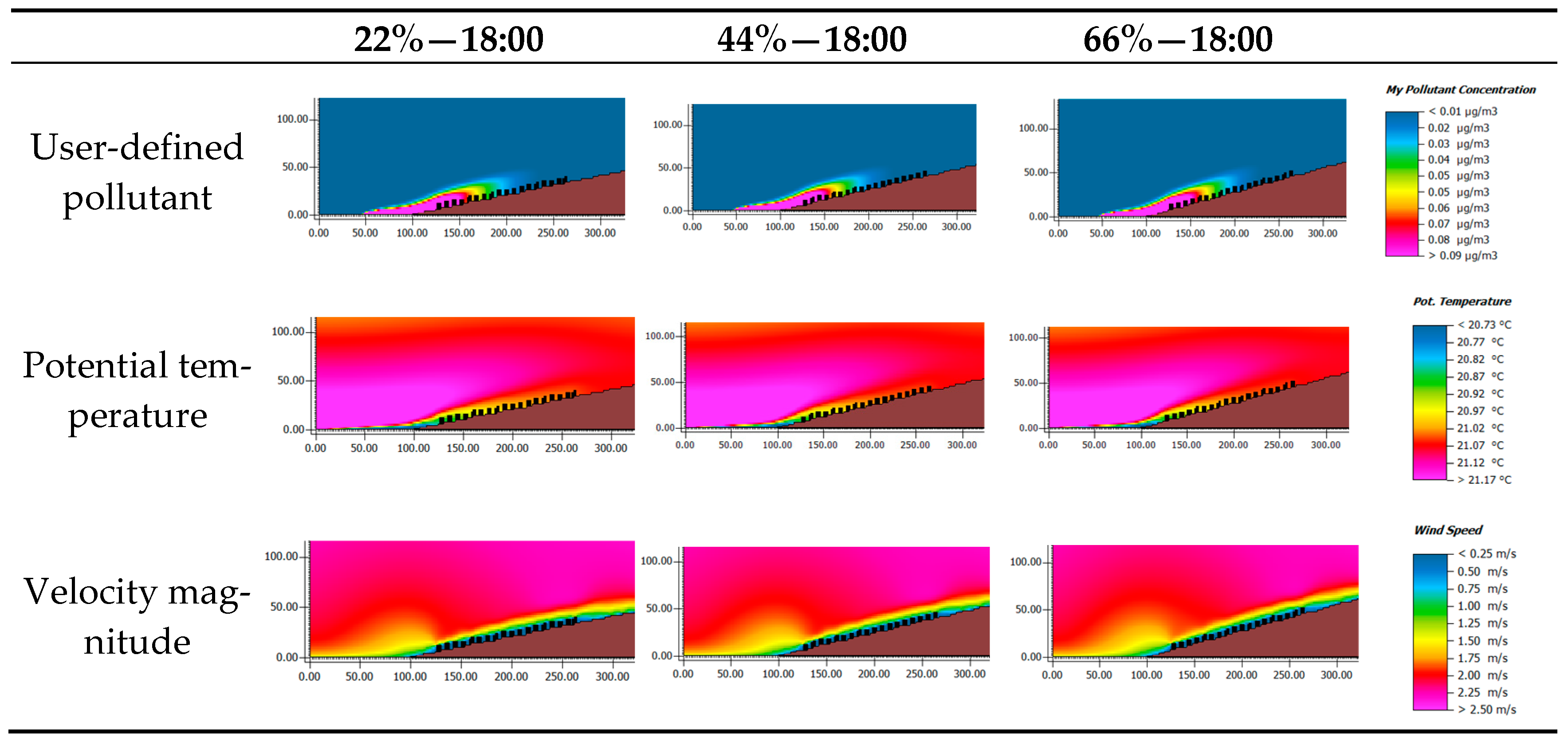
3.2. Influence of Slope

To isolate the influence of slope on air quality, simulations were run with identical building and meteorological conditions, varying only the terrain gradient (22%, 44%, and 66%).

Figure 5 compares pollutant dispersion, thermal stratification, and wind velocity across three slope gradients—22%, 44%, and 66%—at 18:00, under identical building and meteorological conditions. The results reveal a clear progression in flow behavior and pollutant accumulation as slope steepness increases.

In the 22% slope case, the pollutant plume is elongated and dispersed both upslope and vertically. The user-defined scalar extends beyond the midpoint of the slope, aided by moderate wind speeds (1.5–2.0 m/s) and a gradual increase in potential temperature with height (~20.87 °C to ~21.10 °C), which allows for modest vertical mixing. The velocity field shows a continuous upslope flow, enabling advection and dilution.

In contrast, the 44% slope shows a narrower plume that remains closer to the emission source. The potential temperature gradient near the surface becomes sharper, indicating stronger near-ground stability. Wind speeds diminish near the base of the slope and zones of lower velocity (<1.25 m/s) appear behind buildings, suggesting the formation of localized recirculation areas.

In the 66% slope case, pollutant dispersion is sharply restricted. The plume remains confined within the first 50 m of the slope, with the maximum concentrations accumulating at the base. The thermal field displays a well-developed surface inversion and the wind velocity map reveals flow separation and near-stagnant air immediately downstream of the emission source. The presence of pink and red zones in the scalar plot, surrounded by blue wind contours, confirms pollutant trapping in a shallow, stable boundary layer.

These patterns demonstrate that increased slope steepness reduces both horizontal and vertical pollutant transport, amplifying the risk of air quality deterioration in dense hillside settlements. The aerodynamic and thermal effects of topography act together to create low-dispersion zones where pollutants persist near human activity levels.

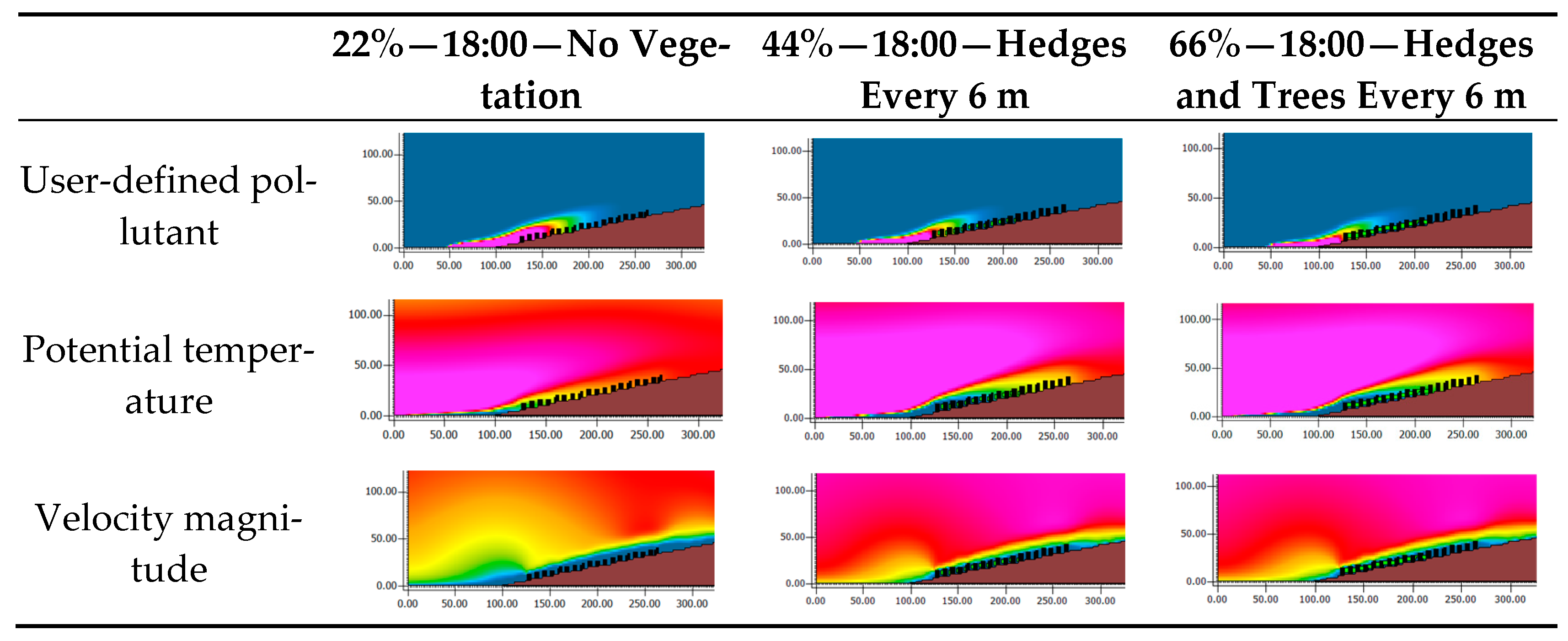
3.3. Vegetation Effect on Pollutant Dispersion

To explore the mitigating role of vegetation, simulations were conducted for three cases with different slope gradients and vegetation types. Figure 6 compares the pollutant concentration, thermal stratification, and wind velocity for (i) a 22% slope without vegetation, (ii) a 44% slope with hedges every 6 m, and (iii) a 66% slope with both hedges and trees.

In the Figure 6, 22% slope case without vegetation, the pollutant plume extends broadly upslope and upward. The concentration field shows a smooth gradient, with lower values near the source and dilution occurring gradually along the slope. The velocity magnitude plot reveals strong, relatively uniform flow (orange and red zones), which supports horizontal transport. The potential temperature profile is moderately stratified, allowing for vertical mixing and minimizing accumulation.

In the 44% slope case with hedges, the dispersion pattern becomes more compact and confined to the lower third of the slope. Vegetation increases aerodynamic drag and creates low-velocity zones near the ground (light blue/green in the wind plot), especially between buildings. Thermal stratification intensifies near the surface, reducing vertical mixing. As a result, pollutants remain trapped in the lower layers, with elevated concentrations close to the emission source.

In the 66% slope case with both trees and hedges, the complexity of the flow field increases. Vegetation introduces localized turbulence and flow disruption, visible in the irregular wind contours behind vegetation elements. However, overall wind speeds remain low (<1.0 m/s) and the thermal field is strongly stable, with sharp temperature gradients that prevent vertical dilution. Pollutants accumulate at the base of the slope, forming a dense, shallow plume adjacent to the built structures.

These results highlight the complex interaction between vegetation, terrain slope, and atmospheric stability. While strategically placed vegetation can enhance local turbulence and mitigate pollutant buildup by disrupting recirculating flow patterns, under steep and thermally stable conditions, it may inadvertently contribute to pollutant entrapment.

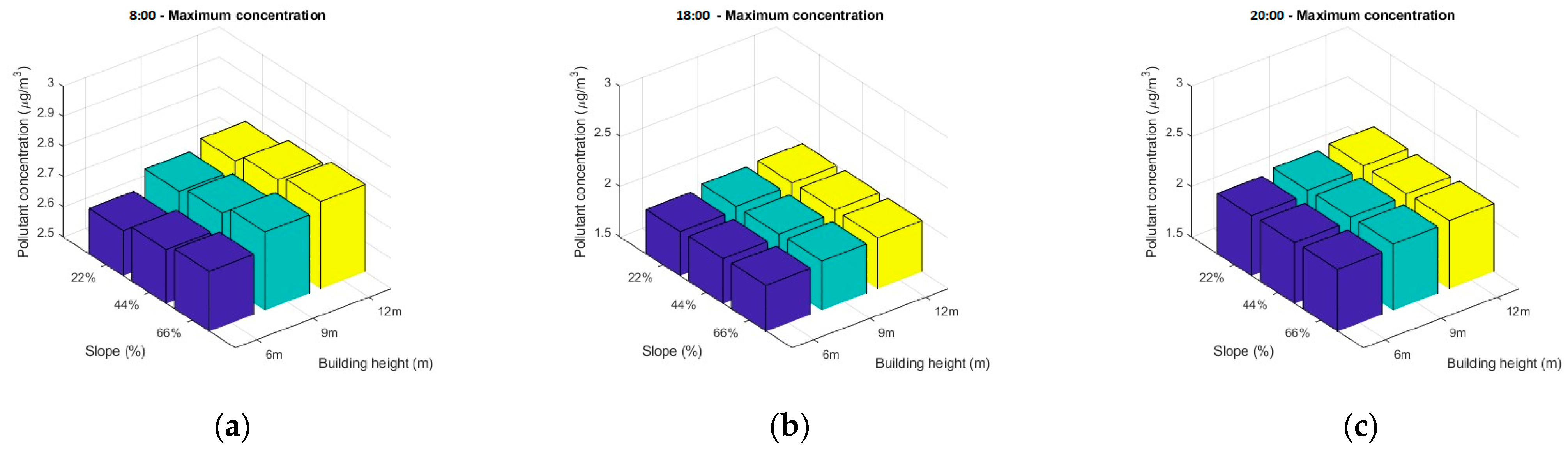
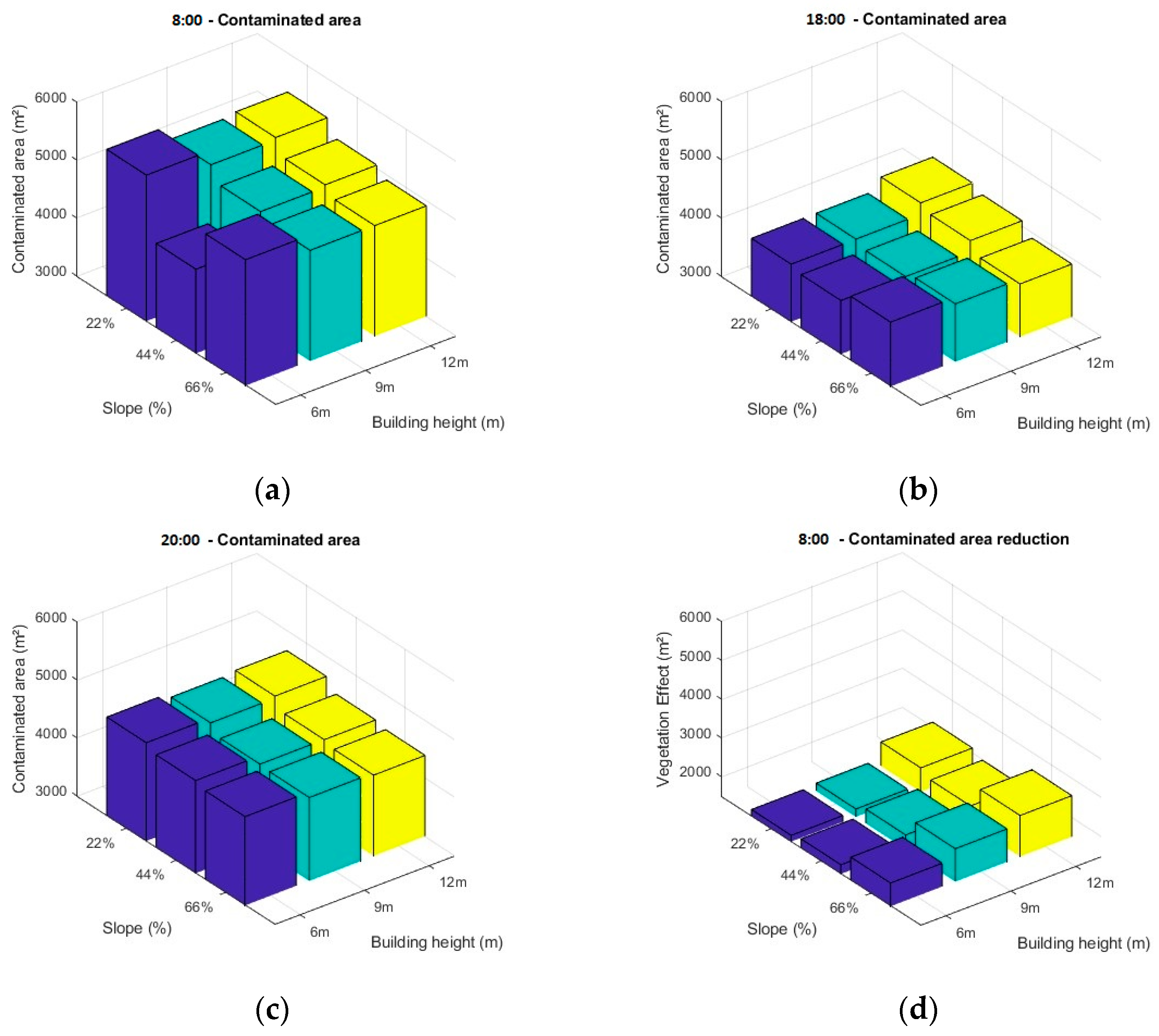
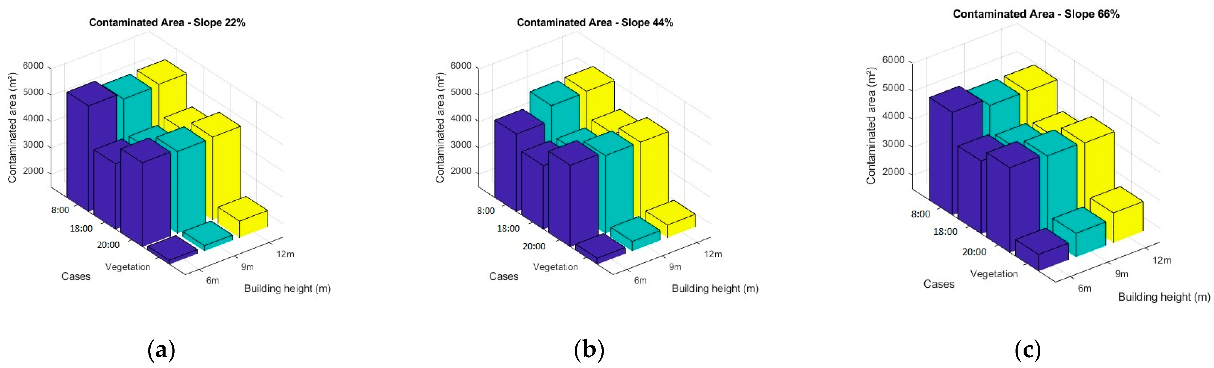
3.4. Quantitative Comparison of Dispersion Scenarios

Figure 7 and Figure 8 provide a comparative analysis of pollutant dispersion as a function of slope angle, building height, and vegetation presence, using the following two key indicators: maximum concentration and contaminated area. Results are presented for three representative times of day: 8:00, 18:00, and 20:00.

Figure 7 shows that the maximum pollutant concentration increases consistently with both slope and building height, regardless of time. The colors in the figure are used solely to distinguish between the different cases and do not represent any specific variable. This pattern is driven by the following two key mechanisms:

(i) Steeper slopes generate larger recirculation zones near the terrain transition, trapping pollutants near the emission source.

(ii) Taller buildings increase surface roughness, decreasing near-ground wind speeds and prolonging the residence time of pollutants within the domain.

In contrast, Figure 8 reveals that the contaminated area decreases as slope and building height increase. This inverse relationship reinforces the idea that pollutants are not dispersing broadly but instead accumulating in more confined, stagnant zones. The effect is most pronounced at 8:00, when higher wind speeds and favorable thermal profiles promote dispersion. At 18:00 and 20:00, atmospheric stability and weaker winds contribute to smaller, concentrated pollution zones.

A fourth subplot (Figure 8d) introduces vegetation at 8:00 (trees and hedges placed every 6 m between buildings). The contaminated area is significantly reduced—comparable to the low-dispersion cases observed at 20:00—suggesting that strategically placed vegetation can partially offset adverse topographic and morphological effects, even during hours with higher transport potential.

3.5. Effectiveness of Vegetation Strategies

To evaluate the role of vegetation in mitigating pollutant dispersion, Figure 9 illustrates the impacts of different vegetation strategies on the contaminated area under the following three slope conditions: 22%, 44%, and 66%.

Across all slope values, the scenario with trees and bushes placed between houses consistently resulted in the most significant reduction in contaminated areas. This configuration increases surface roughness and induces small-scale turbulence, which enhances vertical mixing and decreases pollutant residence time near the ground. Figure 9 shows that this strategy is effective even in steeper terrains, where pollutant accumulation is usually more severe due to recirculation zones.

In contrast, other tested strategies showed varying, generally lower levels of effectiveness. These include the following:

• Trees located at x = 0, positioned near the pollution source;
• Trees of different heights at x = 40, closer to the slope;
• Bushes at x = 40, acting as low green barriers;
• Combined trees and bushes at x = 40, closer to the slope;
• Forest-type vegetation (dense tree formation) at x = 40.

While these configurations offer some reduction in the contaminated area, their effectiveness is limited compared to the between-house vegetation. This observed trend is primarily because vegetation farther from the source may only interact with the pollutant plume after it has already concentrated within low-velocity zones created by the urban morphology and terrain slope.

These results emphasize that the location and type of vegetation play crucial roles. Placing vegetation directly within the pollutant transport path, especially in the inter-building spaces, is key to maximizing pollutant dispersion and minimizing the extent of contamination.

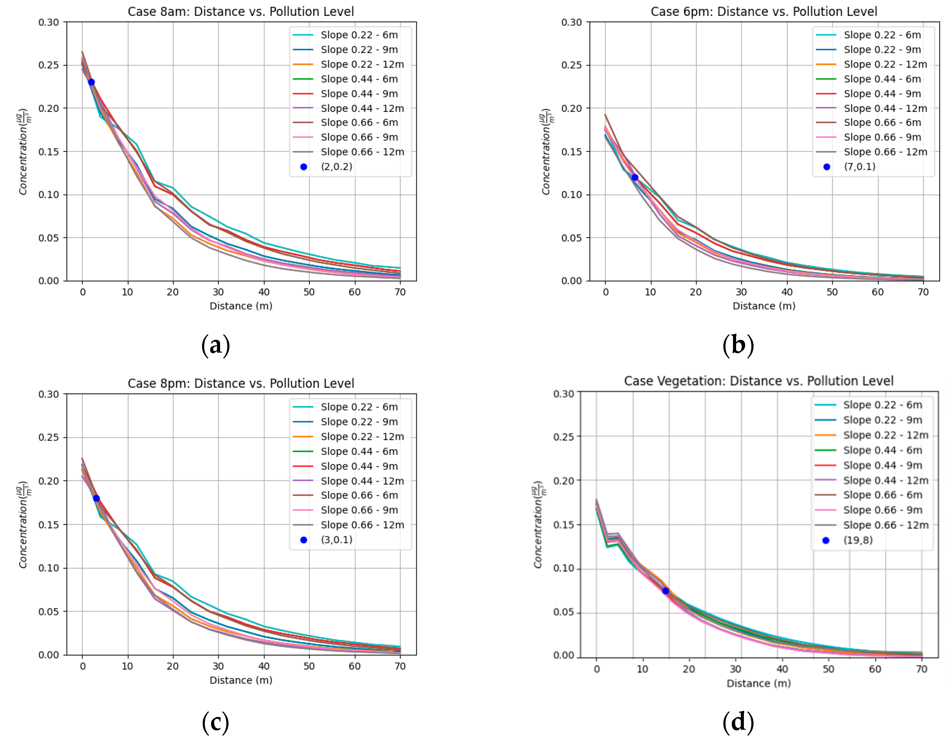
3.6. Pedestrian-Level Pollutant Concentration

Figure 10 presents the pollutant concentration profiles measured at the pedestrian level (i.e., 1.5 m above ground) along the slope for different hours of the day and under different conditions, including vegetation.

At 08:00 (Figure 10a), concentrations are highest, especially near the base of the slope, due to early morning stability and persistent recirculation zones. Steep slopes and taller buildings exacerbate this effect, resulting in peak pedestrian exposure. At 18:00 and 20:00 (Figure 10b,c), concentrations are lower, likely due to slightly enhanced wind and temperature gradients that promote limited vertical dispersion.

An important trend is observed across all cases: concentration levels diverge sharply around 4 m from the emission source, near the location of the first building row. Beyond this point, urban geometry and slope-induced flow structures become dominant, shaping the pollutant pathway.

In Figure 10d, vegetation is introduced at 08:00 using the between-building strategy. The results show a notable reduction in pedestrian-level concentration, reaching levels comparable to the more favorable 20:00 case. This reinforces the finding that vegetation, when well-positioned, can significantly reduce exposure risk during even the most critical hours.

4. Discussion

This study conducted a parametric numerical analysis of pollutant dispersion over idealized hillslope urban geometries, revealing significant interactions between terrain slope, building height, and pollutant concentration patterns. These findings align with previous research emphasizing the role of urban morphology and topography in shaping air quality dynamics.

Although the model setup was simplified to isolate key variables, the slopes (22–66%), building heights (6–12 m), meteorological inputs, and vegetation types used were selected based on their representativeness of actual conditions in hillside districts of Lima, Peru, such as San Juan de Lurigancho and Villa María del Triunfo. This ensures that the analysis, while parametric, maintains strong contextual relevance. Nonetheless, for a more comprehensive understanding of air quality dynamics in these environments, future studies should examine a broader range of slope gradients, building geometries, and vegetation strategies to capture the full variability present in real urban contexts.

Specifically, the observed proportional increase in maximum pollutant concentrations with both slope and building height corroborates the findings reported in [25], which showed that complex urban geometries exacerbate pollutant accumulation in canyon-like structures. Similarly, ref. [26] demonstrated that vertical building configurations strongly influence pollutant dispersion and stagnation zones in dense urban environments. The reduction in the total affected area with an increasing slope suggests a complex trade-off between pollutant intensity and spatial extent, echoing the patterns described in [11] in analyses of pollutant dispersion over complex terrain.

The diurnal variation in pollutant coverage—lower at night than during morning hours—is consistent with established knowledge of atmospheric stability’s effects on dispersion [11,27]. As documented in various urban meteorological studies, stable nighttime conditions reduce vertical mixing, while daytime turbulence promotes dispersion. This is aligned with recent findings that highlight the significant influence of urban canopy resistance and ventilation obstruction on PM_2.5 accumulation, particularly under conditions of limited atmospheric mixing [28].

Vegetation’s role as a modulator of pollutant concentration, particularly the beneficial impact of trees and hedges spaced at approximately the building height scale (~6 m), agrees with [29], which quantified urban vegetation’s capacity to reduce air pollution via deposition and altered airflow. However, studies such as [30] highlight that vegetation effects are site-specific and must be carefully evaluated within the local urban and meteorological context to avoid unintended microclimatic consequences, such as reduced ventilation or pollutant trapping. This is further supported by the findings in [31], where computational fluid dynamics (CFD) simulations demonstrated that roadside vegetation—especially dense tree canopies—can lead to increased local pollutant concentrations due to impaired air circulation. The authors concluded that, in many cases, the aerodynamic disruption caused by vegetation outweighs its pollutant removal benefits.

Topographic influences on wind flow, including flow separation, downslope gravity currents, and vortex formation, add complexity to pollutant transport dynamics. Recent work in [31] supports this, arguing that Reynolds-Averaged Navier–Stokes (RANS) models have inherent limitations in capturing these nonlinear flow phenomena over steep terrain and recommending large eddy simulations (LESs) for an improved representation of buoyancy-driven turbulence and flow separation effects.

This study’s limitations—such as a single wind direction perpendicular to the slope, an idealized infinite domain, and the absence of seasonal variability—are common in parametric modeling, but restrict direct real-world applicability. Future research should extend to multiple wind directions and speeds, seasonal meteorological changes, and variable pollutant sources to more realistically capture urban air quality dynamics [32,33]. Furthermore, it is essential to address the dynamic interactions between micro- and macro-scales in urban atmospheric processes. As highlighted in [34], a persistent gap remains in our ability to effectively bridge these scales, which significantly hampers the development of integrated and accurate air quality modeling frameworks.

Moreover, integrating pedestrian comfort and health risk assessments, as proposed in [35], will enhance the societal relevance of modeling outcomes. Validating model predictions with field measurements in actual hillslope urban areas is crucial to confirm and refine simulation results, as emphasized in the validation efforts.

Finally, it is important to clarify that while this study identifies a proportional relationship between building height and increased pollutant concentrations under specific topographic and meteorological conditions, these findings should not be interpreted as prescriptive recommendations regarding optimal urban form. Taller buildings, particularly in hillside districts, may also reflect positive socioeconomic factors such as increased investment in infrastructure, better access to services, or higher housing quality. Therefore, urban design decisions must balance air quality considerations with broader development goals, including social equity, economic opportunity, and spatial efficiency.

5. Conclusions

This parametric study advances our understanding of how terrain slope, building height, urban morphology, and vegetation interact to influence pollutant dispersion in hillslope urban environments. The results reveal that steeper slopes and taller buildings are associated with increased peak pollutant concentrations, yet a concurrent reduction in the spatial extent of affected areas suggests a complex interplay between pollutant intensity and distribution. These dynamics emphasize the critical role of topography and built form in shaping local air quality, particularly in densely populated, sloped urban districts.

Vegetation emerges as a double-edged tool: while appropriately placed trees and hedges, especially at scales comparable to building height, can reduce pollutant concentrations through deposition and airflow modulation, their effectiveness is highly context-dependent. Poorly planned vegetation may inadvertently obstruct ventilation, highlighting the need for site-specific design and evaluation.

The findings underscore the necessity of integrating fine-scale topographic and morphological features into urban air quality models to enhance predictive capacity in complex terrains. While Reynolds-Averaged Navier–Stokes (RANS) models like ENVI-met offer computational efficiency, their limitations in simulating turbulent and buoyancy-driven flows suggest the value of incorporating large eddy simulations (LESs) in future studies for improved accuracy.

The study’s constraints—such as a fixed wind direction and simplified meteorological inputs—point to the importance of broader simulations that include variable climatic conditions, pollutant sources, and human activity patterns. Expanding these parameters will improve model robustness and real-world applicability.

Ultimately, this research provides a foundation for developing targeted urban planning and green infrastructure strategies tailored to the unique challenges of hillslope settlements. By illuminating the interdependent roles of slope, building configuration, and vegetation, it offers actionable insights to guide interventions that enhance air quality while balancing socioeconomic development. A multidisciplinary, context-sensitive approach—combining advanced modeling, empirical validation, and urban design—is essential to foster healthier, more resilient cities in steep terrain.