
Study of the Optimal Control of the Central Air Conditioning Cooling Water System for a Deep Subway Station in Chongqing


Abstract
1. Introduction
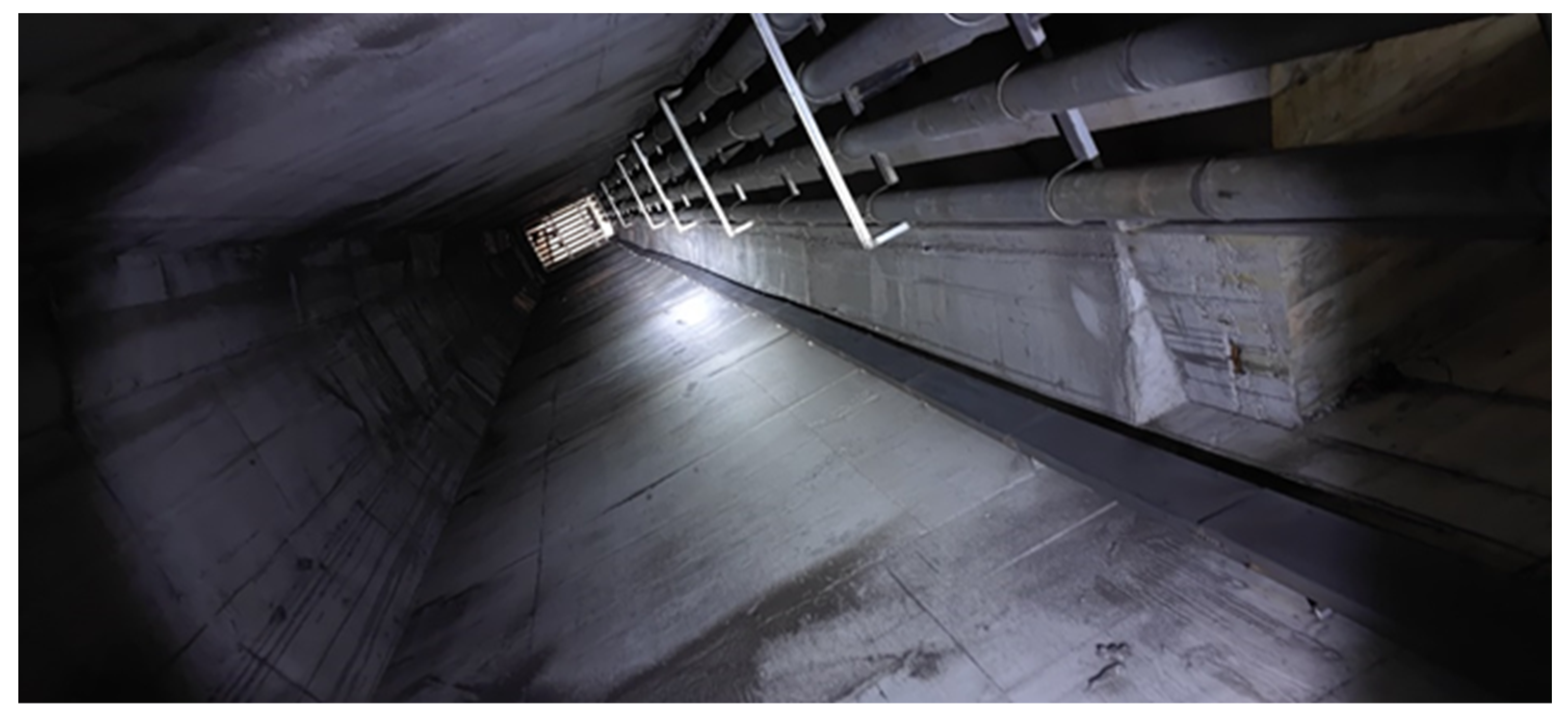
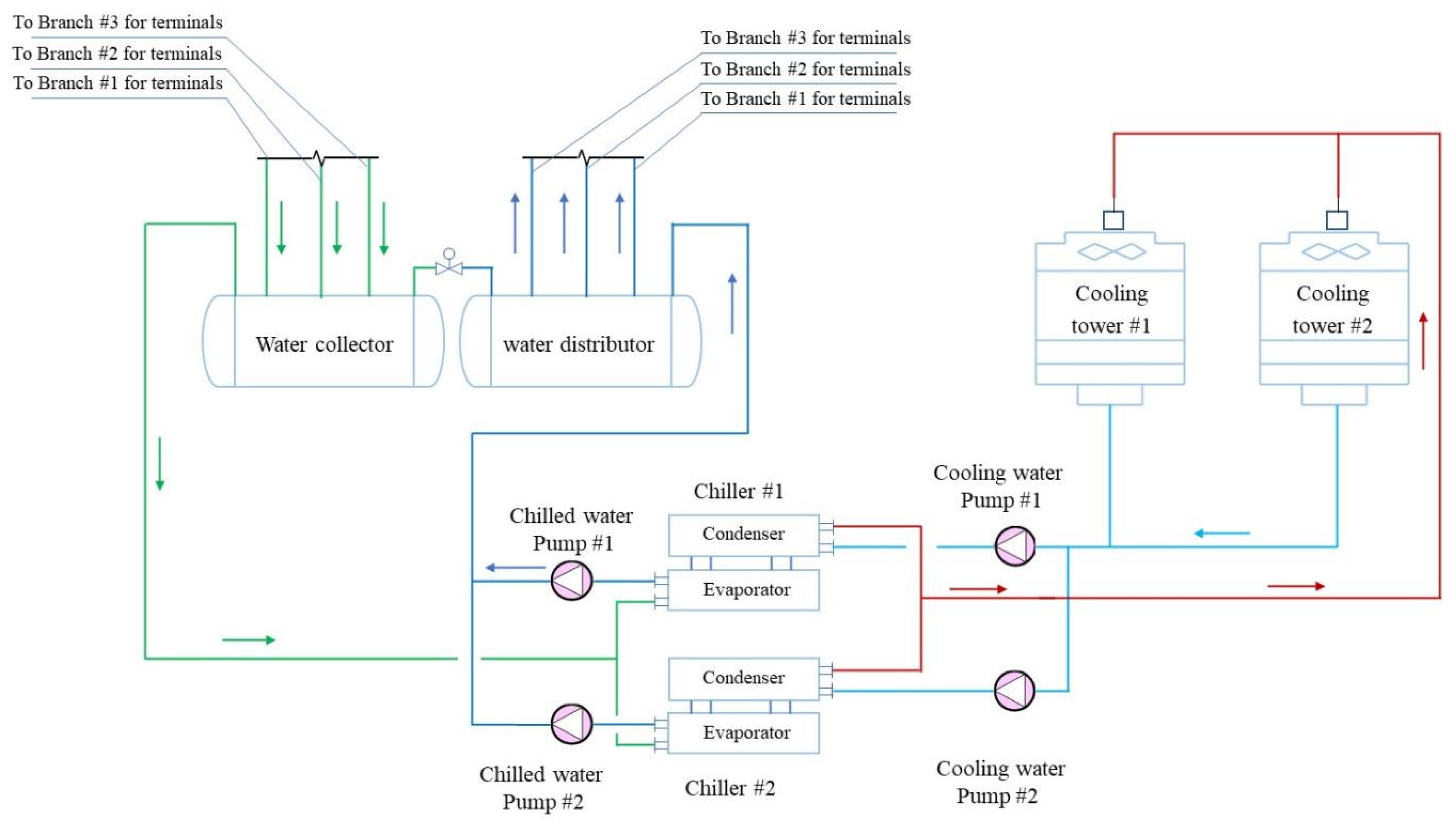
2. System Overview
3. Strategy for Optimal Control of Condenser Inlet Cooling Water Temperature
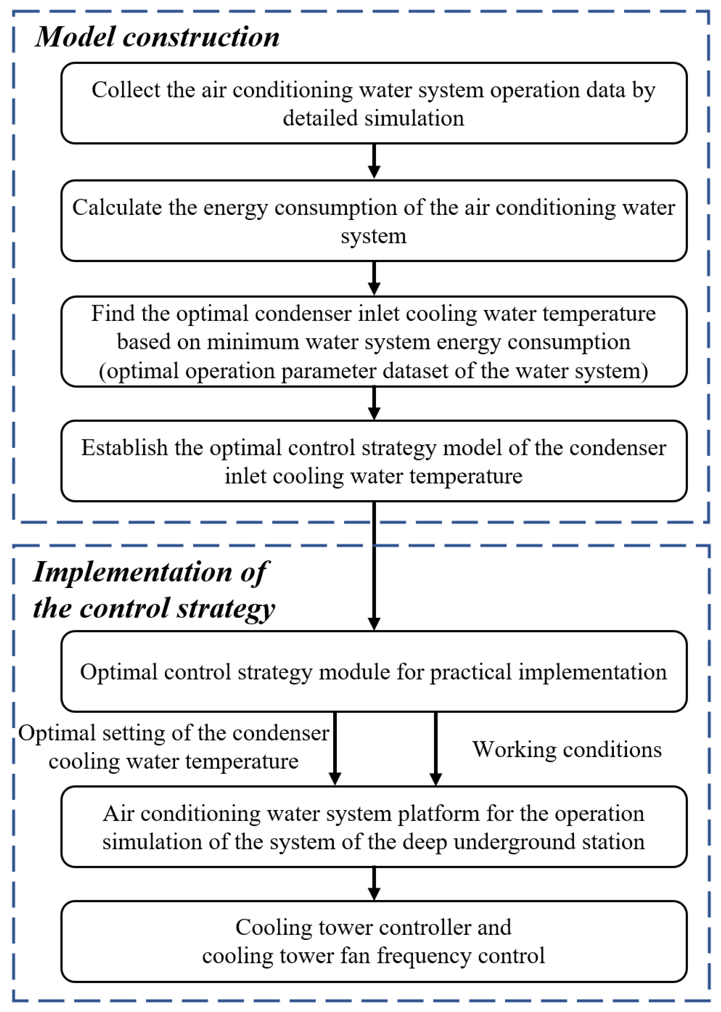
3.1. Concept and Flowchart of Strategy
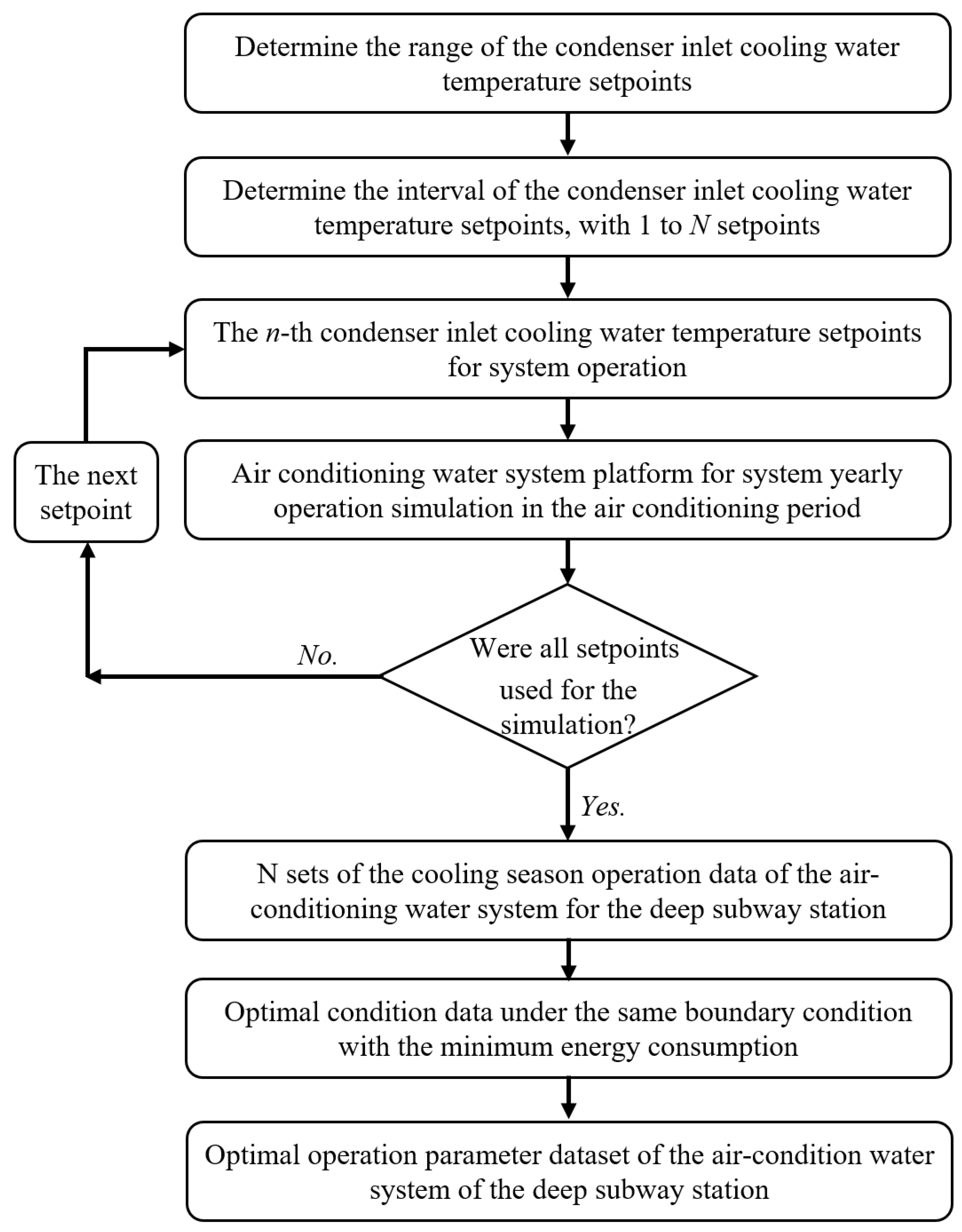
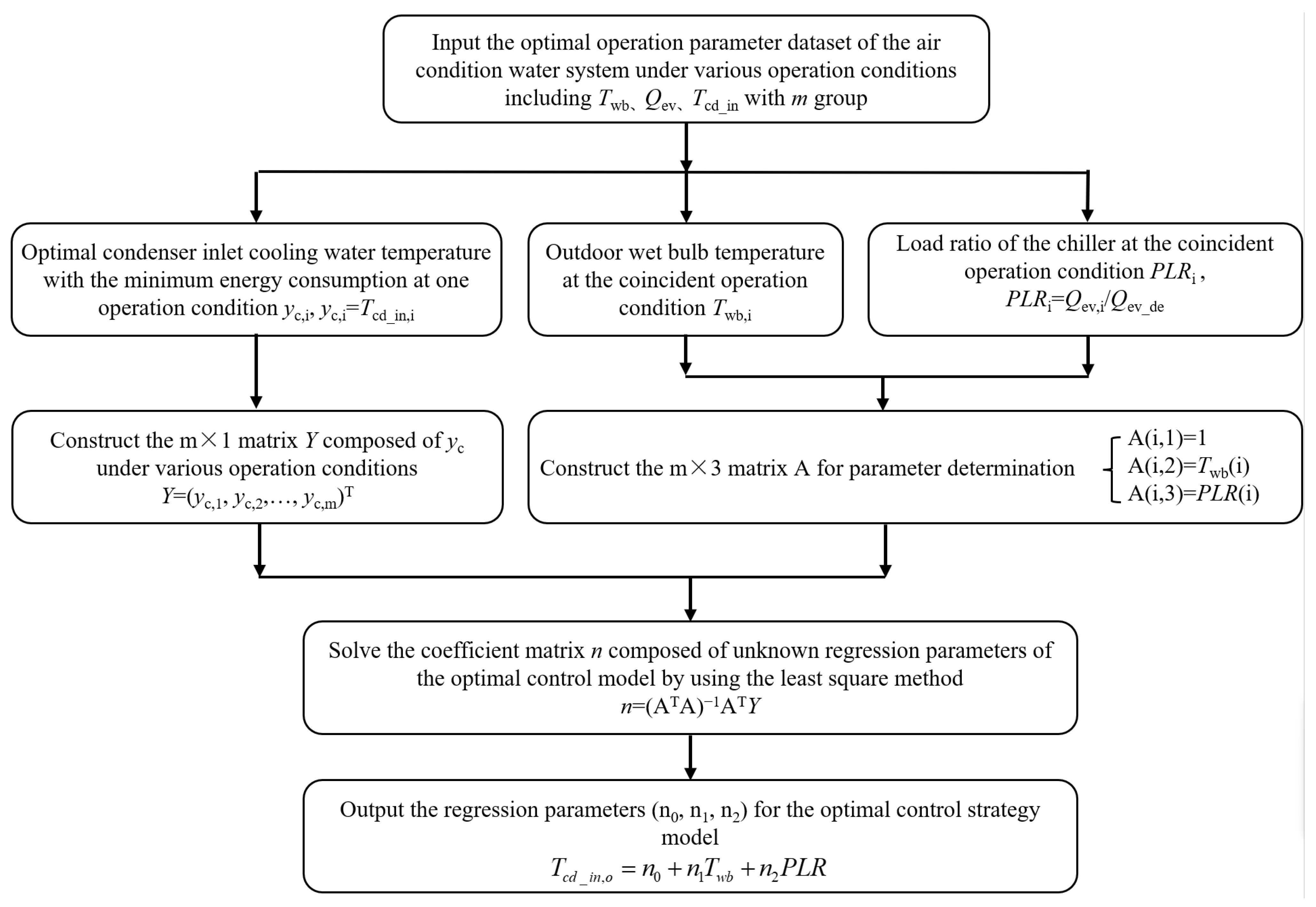
3.2. Control Strategy Model and Flowchart of Parameter Determination
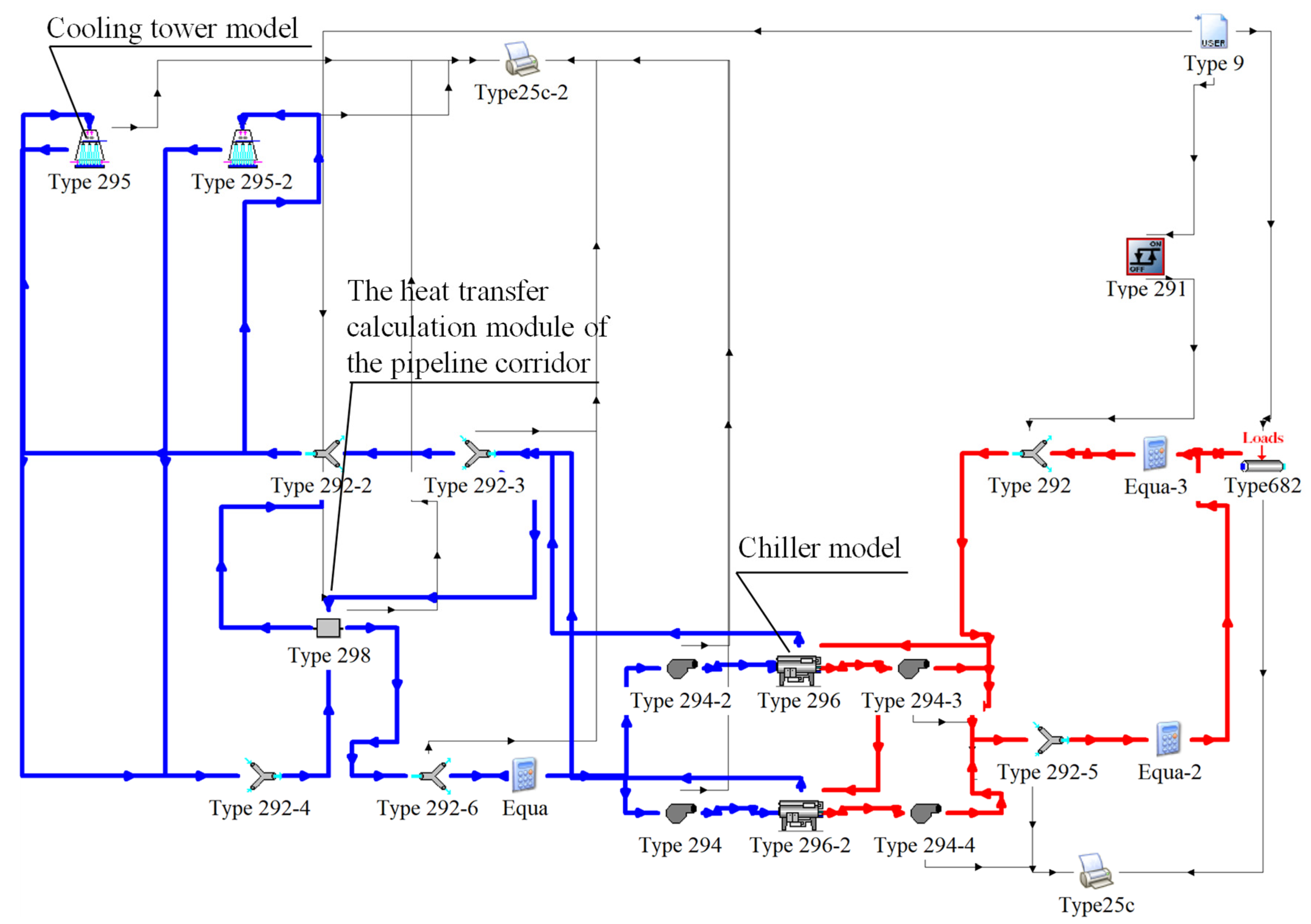
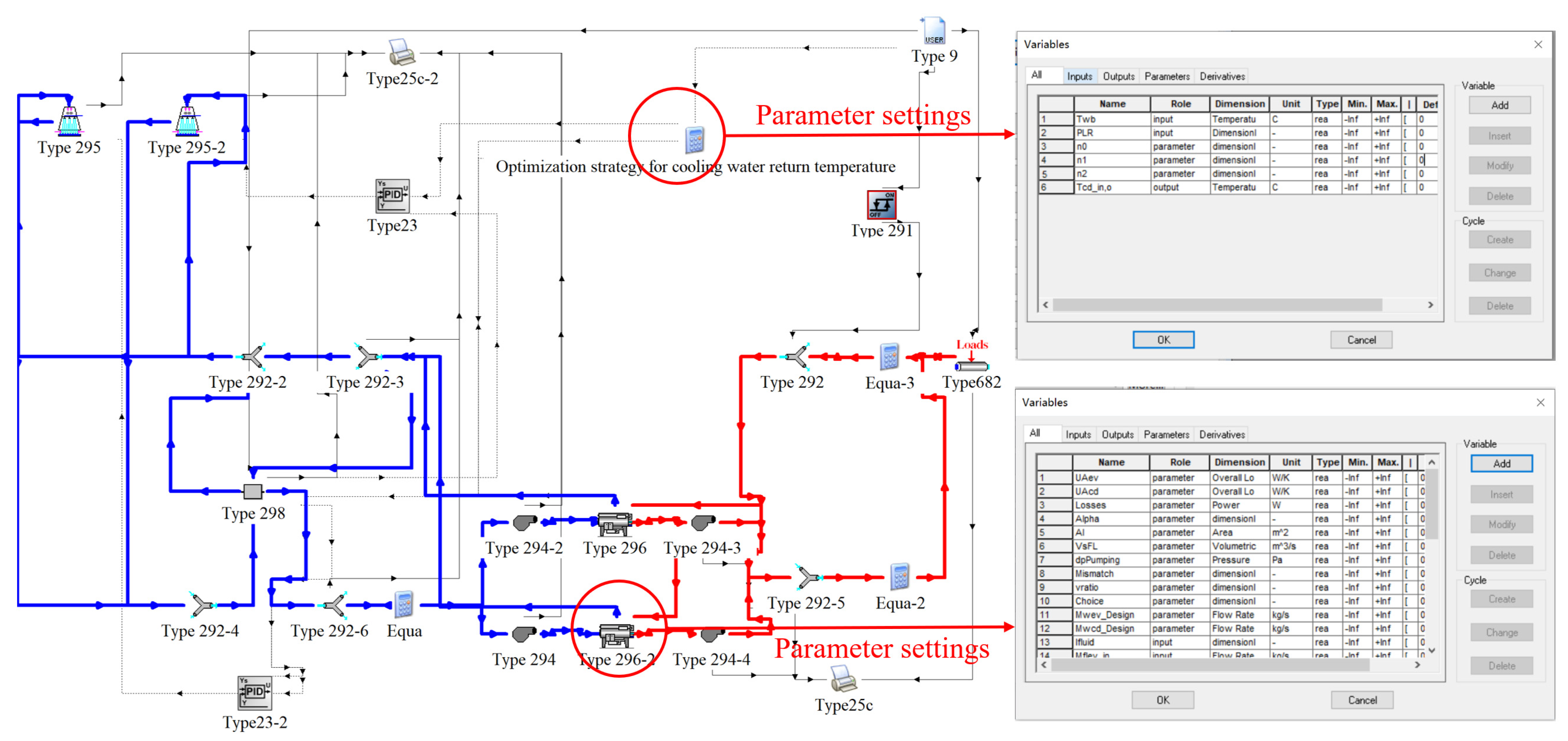
4. Simulation Platform of AC Water System
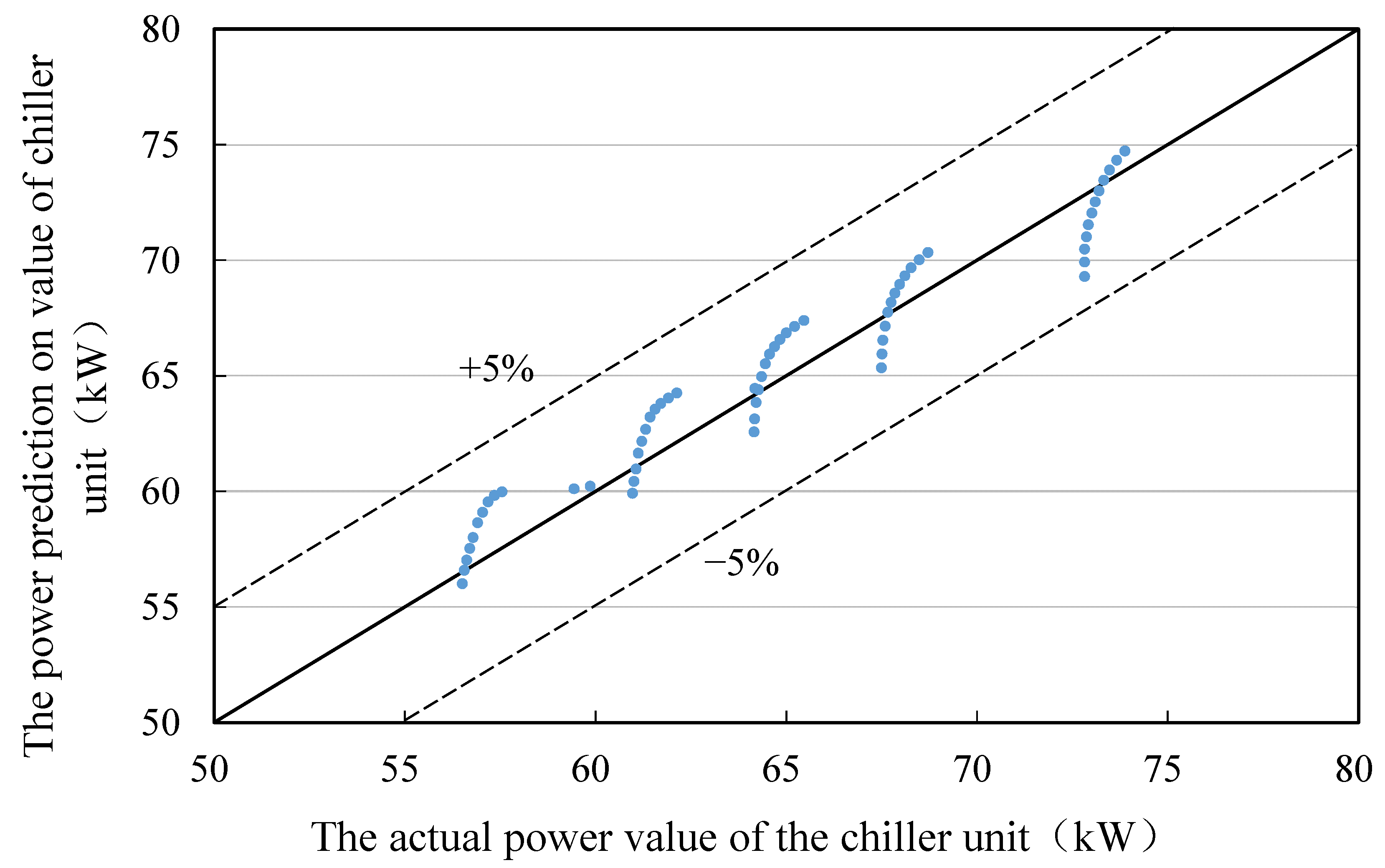
4.1. Chiller Model
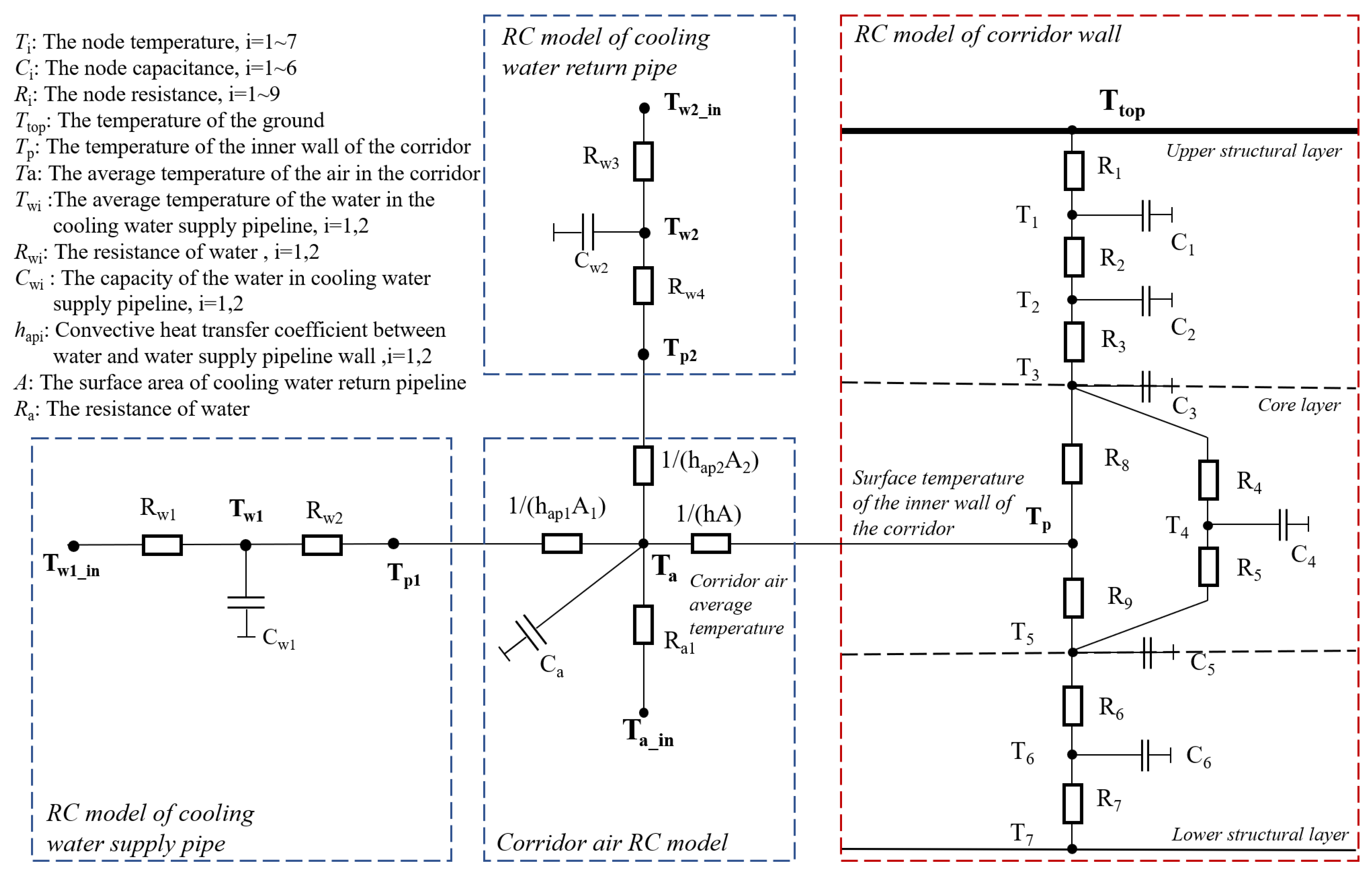
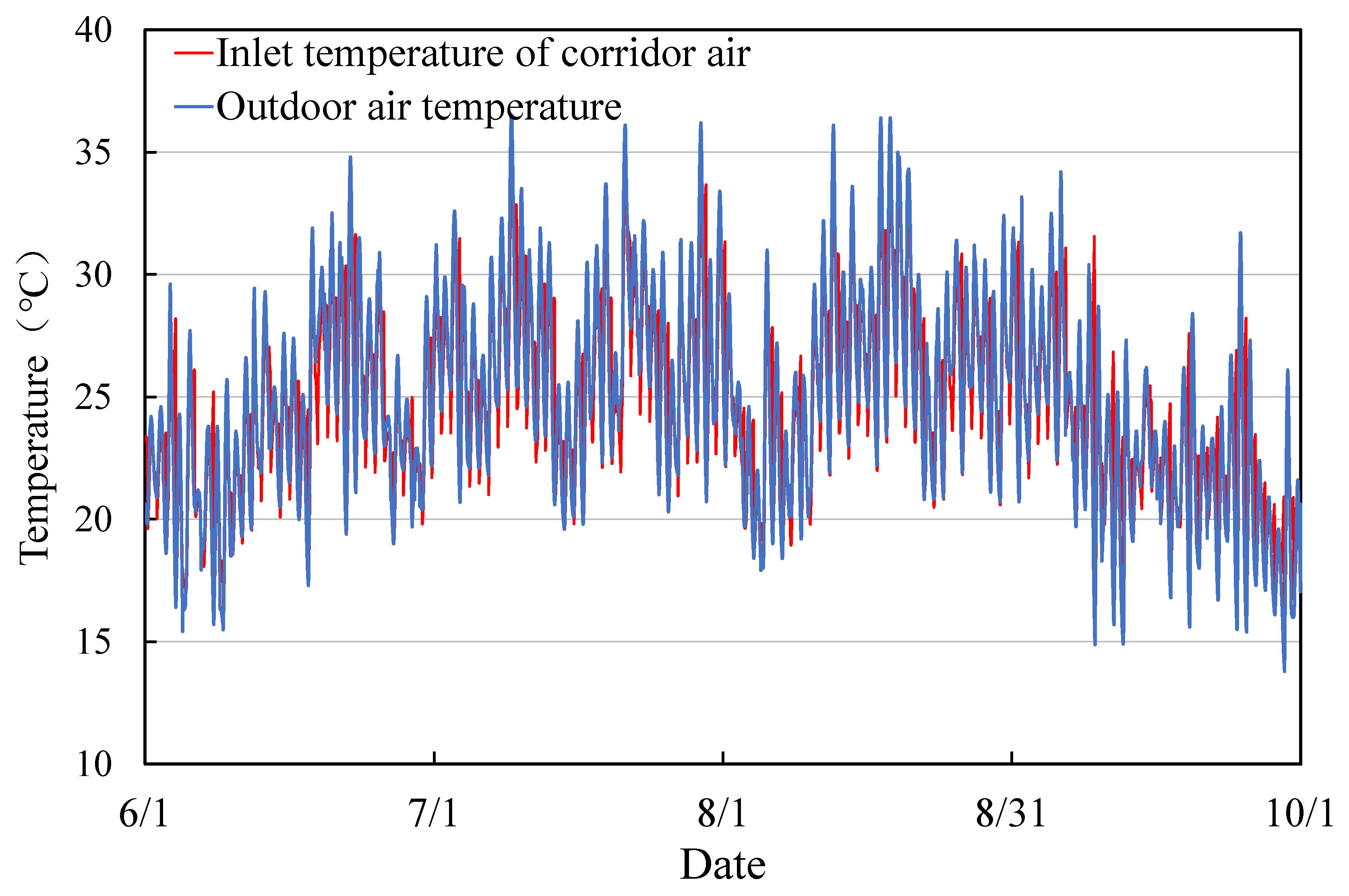
4.2. A Heat Transfer Model of the Pipeline in the Corridor
4.3. Cooling Tower Model
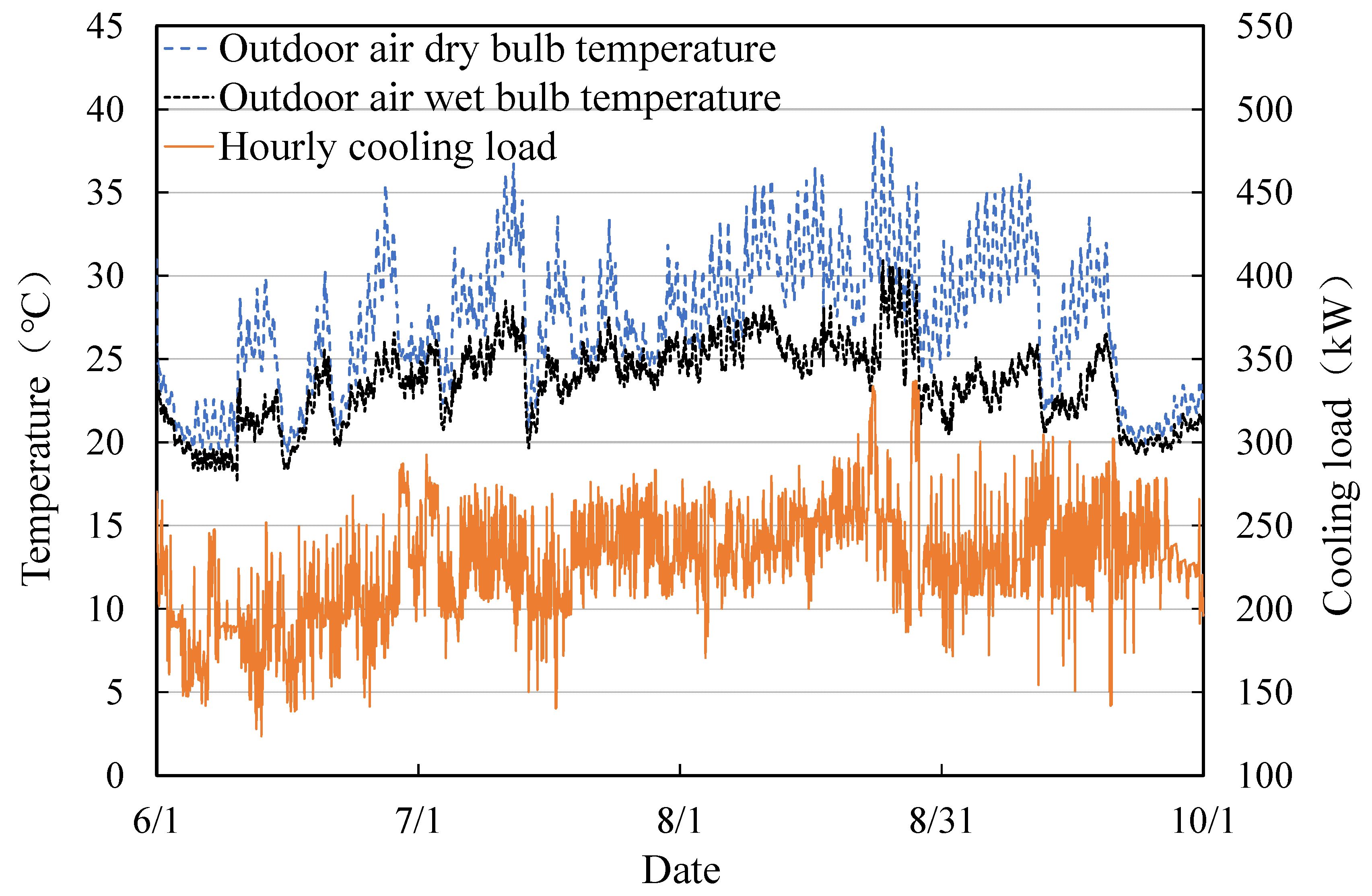
4.4. Simulation Platform
5. Parameters of Optimal Control Strategy
6. Implementation of Optimal Control Strategy and Result Analysis
6.1. Implementation Architecture of Optimal Control Strategy
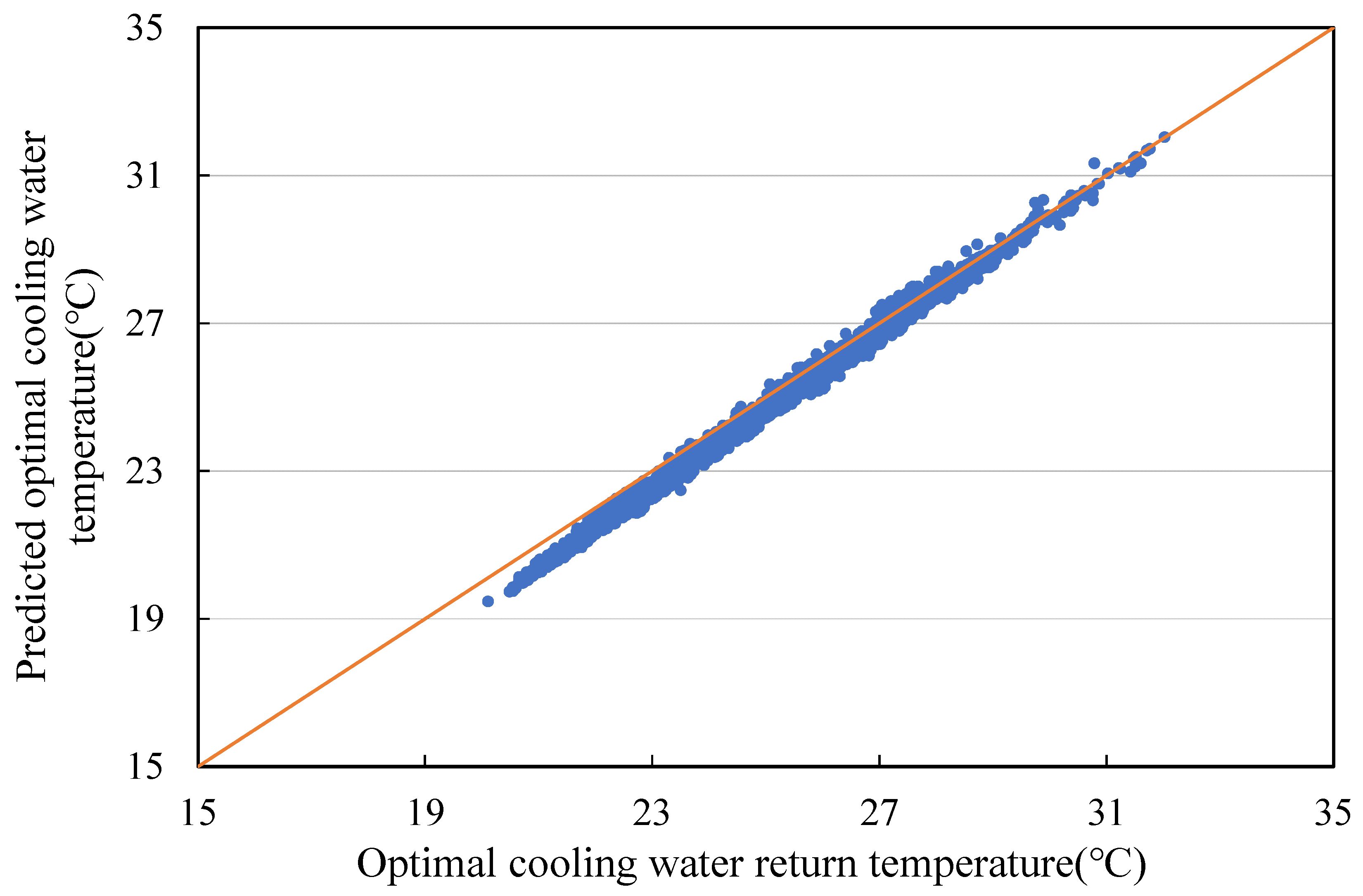
6.2. The Control and Thermal Results of Online Implementation of the Strategy
6.3. Energy Efficiency Evaluation
7. Conclusions
Author Contributions
Funding
Data Availability Statement
Conflicts of Interest
List of Main Symbols
| Symbol | Meaning | Unit |
| AC | Air conditioning | - |
| E | Energy consumption | - |
| n0~2 | Fitting coefficients | - |
| PLR | Cooling load ratio of the chiller | - |
| W | Power | W |
| Qev | Chiller cooling capacity | W |
| h | Enthalpy value | J/kg |
| MR | Mass refrigerant flow rate | g/s |
| α | Loss coefficient | - |
| C | Heat capacity | J/K |
| T | Temperatrue | °C |
| R | Value of resistance | W/(m2·K) |
Subscript
| Symbol | Meaning | Symbol | Meaning |
| a | Air | p | Corridor wall |
| CT | Cooling tower | p1 | Cooling water supply pipe wall |
| cd | Condenser | p2 | Cooling water return pipe wall |
| chw | Chilled water | w | Water |
| ev | Evaporator | w1 | Cooling water supply pipe |
| in | Inlet | w2 | Cooling water return pipe |
| lo | Loss | wb | Wet bulb temperature |
| max | Maximum | 1 | Evaporator outlet point |
| min | Minimum | 2 | Condenser inlet point |
| out | Outlet |
References
- Yu, N.; Wang, Y.; Zhou, Y.; Hu, Y.; Wu, J.; Zhang, L. Field Study and Analysis of Passenger Density in the Beijing Subway Transfer Hall. Buildings 2024, 14, 2504. [Google Scholar] [CrossRef]
- Yang, Z.; Yu, Z.; Yu, L.; Ma, F. Research on frequency conversion technology of metro station’s ventilation and air-conditioning system. Appl. Therm. Eng. 2014, 69, 123–129. [Google Scholar] [CrossRef]
- Zhong, H.; Wang, J.; Chen, C.; Wang, J.; Li, D.; Guo, K. Weather Interaction-Aware Spatio-Temporal Attention Networks for Urban Traffic Flow Prediction. Buildings 2024, 14, 647. [Google Scholar] [CrossRef]
- U I D T Publics(Uitp), World Metro Figures 2021, 2022. Available online: https://www.uitp.org/publications/metro-world-figures-2021/ (accessed on 22 September 2024).
- Su, Z.; Li, X. Sub-system energy model based on actual operation data for subway stations. Sustain. Cities Soc. 2020, 52, 101835. [Google Scholar] [CrossRef]
- Chen, Z.; Xie, X.; Hu, H.; Zhou, X.; Yang, Y.; Song, W.; Luh, D.B.; Li, X. Field investigation on thermal comfort of metro passengers in hot summer and warm winter zone of China: A case study in Guangzhou. Energy Build. 2024, 320, 114633. [Google Scholar] [CrossRef]
- Chen, L.W.M.; He, L.; Wang, G.; Xia, S. Study on Early Warning Model in Energy Consumption of Metro VAC Water. Urban Rail Transit Res. 2022, 25, 36–39. (In Chinese) [Google Scholar]
- Angrisani, G.; Minichiello, F.; Sasso, M. Improvements of an unconventional desiccant air conditioning system based on experimental investigations. Energy Convers. Manag. 2016, 112, 423–434. [Google Scholar] [CrossRef]
- Mossolly, M.; Ghali, K.; Ghaddar, N. Optimal control strategy for a multi-zone air conditioning system using a genetic algorithm. Energy 2009, 34, 58–66. [Google Scholar] [CrossRef]
- Wang, X.; Liu, K.; You, W.; Zhang, X.; Ma, H. Stepwise Optimization Method of Group Control Strategy Applied to Chiller Room in Cooling Season. Buildings 2023, 13, 487. [Google Scholar] [CrossRef]
- Zhou, X.; Wang, B.; Liang, L.; Yan, J.; Pan, D. An operational parameter optimization method based on association rules mining for chiller plant. J. Build. Eng. 2019, 26, 100870. [Google Scholar] [CrossRef]
- Zhang, Y.; Wei, Z.; Zhang, M. Free cooling technologies for data centers: Energy saving mechanism and applications. Energy Procedia 2017, 143, 410–415. [Google Scholar] [CrossRef]
- Dong, K.; Li, P.; Huang, Z.; Su, L.; Sun, Q. Research on Free Cooling of Data Centers by Using Indirect Cooling of Open Cooling Tower. Procedia Eng. 2017, 205, 2831–2838. [Google Scholar] [CrossRef]
- Eidan, A.A.; Alwan, K.J.; AlSahlani, A.; Alfahham, M. Enhancement of the Performance Characteristics for Air-Conditioning System by Using Direct Evaporative Cooling in Hot Climates. Energy Procedia 2017, 142, 3998–4003. [Google Scholar] [CrossRef]
- Fang, Z.; Tang, T.; Su, Q.; Zheng, Z.; Xu, X.; Ding, Y.; Liao, M. Investigation into optimal control of terminal unit of air conditioning system for reducing energy consumption. Appl. Therm. Eng. 2020, 177, 115499. [Google Scholar] [CrossRef]
- Yang, S.; Yu, J.; Gao, Z.; Zhao, A. Energy-saving optimization of air-conditioning water system based on data-driven and improved parallel artificial immune system algorithm. Energy Convers. Manag. 2023, 283, 116902. [Google Scholar] [CrossRef]
- Lu, L.; Cai, W.; Soh, Y.C.; Xie, L.; Li, S. HVAC system optimization––condenser water loop. Energy Convers. Manag. 2004, 45, 613–630. [Google Scholar] [CrossRef]
- Karami, M.; Wang, L. Particle Swarm optimization for control operation of an all-variable speed water-cooled chiller plant. Appl. Therm. Eng. 2018, 130, 962–978. [Google Scholar] [CrossRef]
- Ma, K.; Liu, M.; Zhang, J. Online optimization method of cooling water system based on the heat transfer model for cooling tower. Energy 2021, 231, 120896. [Google Scholar] [CrossRef]
- Sun, J.; Reddy, A. Optimal control of building HVAC&R systems using complete simulation-based sequential quadratic programming (CSB-SQP). Build. Environ. 2005, 40, 657–669. [Google Scholar]
- Ma, Z.; Wang, S.; Xu, X.; Xiao, F. A supervisory control strategy for building cooling water systems for practical and real time applications. Energy Convers. Manag. 2008, 49, 2324–2336. [Google Scholar] [CrossRef]
- Ma, K.; Liu, M.; Zhang, J. A method for determining the optimum state of recirculating cooling water system and experimental investigation based on heat dissipation efficiency. Appl. Therm. Eng. 2020, 176, 115398. [Google Scholar] [CrossRef]
- Zhang, H.; Cui, T.; Liu, M.; Zheng, W.; Zhu, C.; You, S.; Zhang, Y. Energy performance investigation of an innovative environmental control system in subway station. Build. Environ. 2017, 126, 68–81. [Google Scholar] [CrossRef]
- Zhu, N.; Shan, K.; Wang, S.; Sun, Y. An optimal control strategy with enhanced robustness for air-conditioning systems considering model and measurement uncertainties. Energy Build. 2013, 67, 540–550. [Google Scholar] [CrossRef]
- Wang, J.; Wang, S.; Xu, X.; Xiao, F. Evaluation of alternative arrangements of a heat pump system for plume abatement in a large-scale chiller plant in a subtropical region. Energy Build. 2009, 41, 596–606. [Google Scholar] [CrossRef]
- Ashrae. HVAC Systems and Equipment. In ASHRAE Handbook; Stephen Comstock: Atlanta, GA, USA, 1992. [Google Scholar]
- Pillis, J.W. Design and Application of Variable Volume Ratio Screw Compressor. ASHRAE Trans. 1985, 91, 289–296. [Google Scholar]


| Cooling load 190 kW | |||||||
| Outdoor air wet bulb temperature (°C) | 19.6 | 21.7 | 22.9 | 23.2 | 24.5 | 25.6 | 26.7 |
| Minimum E of the water system (kWh) | 68.3 | 70.4 | 71.7 | 72.2 | 73.5 | 74.7 | 76.0 |
| Optimal condenser inlet cooling water temperature (°C) | 21.8 | 23.6 | 24.8 | 25.1 | 26.2 | 27.1 | 28.2 |
| Cooling load 270 kW | |||||||
| Outdoor air wet bulb temperature (°C) | 19.6 | 21.7 | 22.9 | 23.5 | 24.4 | 25.6 | 26.7 |
| Minimum energy consumption of the water system (kWh) | 78.7 | 80.9 | 82.6 | 83.5 | 84.5 | 86.4 | 87.6 |
| Optimal condenser inlet cooling water temperature (°C) | 22.1 | 23.9 | 24.9 | 25.5 | 26.2 | 27.4 | 28.2 |
| Setpoint (°C) | Condenser Inlet Cooling Water Temperature (°C) | Frequency (Hz) | Fan Energy Consumption (kWh) | Chiller Energy Consumption (kWh) | Total Energy Consumption of the Air Conditioning System (kWh) | Water System COP |
|---|---|---|---|---|---|---|
| 25.6 | 26.28 | 50.00 | 6.49 | 42.06 | 78.55 | 2.41 |
| 25.7 | 26.29 | 50.00 | 6.49 | 42.06 | 78.55 | 2.41 |
| 25.8 | 26.29 | 50.00 | 6.49 | 42.06 | 78.55 | 2.41 |
| 25.9 | 26.31 | 50.00 | 6.49 | 42.09 | 78.58 | 2.41 |
| 26.0 | 26.37 | 46.54 | 5.38 | 42.16 | 77.54 | 2.45 |
| 26.1 | 26.43 | 43.37 | 4.50 | 42.24 | 76.74 | 2.47 |
| 26.2 | 26.49 | 40.58 | 3.83 | 42.32 | 76.15 | 2.49 |
| 26.3 | 26.56 | 38.12 | 3.30 | 42.41 | 75.71 | 2.51 |
| 26.4 | 26.64 | 35.93 | 2.88 | 0.04 | 75.38 | 2.52 |
| 26.5 | 26.71 | 33.98 | 2.55 | 42.59 | 75.14 | 2.52 |
| 26.6 | 26.79 | 32.24 | 2.27 | 42.69 | 74.96 | 2.53 |
| 26.7 | 26.87 | 30.67 | 2.05 | 42.80 | 74.84 | 2.53 |
| 26.8 | 26.96 | 29.25 | 1.86 | 42.90 | 74.76 | 2.54 |
| 26.9 | 27.04 | 27.96 | 1.70 | 43.01 | 74.71 | 2.54 |
| 27.0 | 27.13 | 26.79 | 1.56 | 43.12 | 74.68 | 2.54 |
| 27.1 | 27.22 | 25.72 | 1.44 | 43.23 | 74.67 | 2.54 |
| 27.2 | 27.31 | 24.74 | 1.34 | 43.35 | 74.69 | 2.54 |
| 27.3 | 27.40 | 23.84 | 1.25 | 43.46 | 74.71 | 2.54 |
| 27.4 | 27.49 | 23.01 | 1.17 | 43.58 | 74.75 | 2.54 |
| 27.5 | 27.59 | 22.23 | 1.10 | 43.70 | 74.80 | 2.54 |
| 27.6 | 27.68 | 21.48 | 1.03 | 43.83 | 74.86 | 2.53 |
| 27.7 | 27.78 | 20.73 | 0.97 | 43.95 | 74.91 | 2.53 |
| 27.8 | 27.83 | 20.12 | 0.92 | 44.01 | 74.93 | 2.53 |
| 27.9 | 27.83 | 20.00 | 0.91 | 44.01 | 74.92 | 2.53 |
| 28.0 | 27.83 | 20.00 | 0.91 | 44.01 | 74.92 | 2.53 |
| Energy Consumption (kWh) | June | July | August | September |
|---|---|---|---|---|
| Existing mode | 53,887 | 61,630 | 64,303 | 58,071 |
| Optimal mode | 51,527 | 59,112 | 61,770 | 55,702 |
| Energy-saving | 2360 | 2518 | 2533 | 2369 |
| Energy-saving rate | 4.4% | 4.1% | 3.9% | 4.1% |
| Energy Consumption (kWh) | Chiller | Cooling Tower Fan | Entire Water System |
|---|---|---|---|
| Existing Mode | 131,000 | 19,020 | 237,890 |
| Optimized Mode | 133,408 | 6834 | 228,112 |
| Saving amount | −2408 | 12,186 | 9778 |
Disclaimer/Publisher’s Note: The statements, opinions and data contained in all publications are solely those of the individual author(s) and contributor(s) and not of MDPI and/or the editor(s). MDPI and/or the editor(s) disclaim responsibility for any injury to people or property resulting from any ideas, methods, instructions or products referred to in the content. |
© 2024 by the authors. Licensee MDPI, Basel, Switzerland. This article is an open access article distributed under the terms and conditions of the Creative Commons Attribution (CC BY) license (https://creativecommons.org/licenses/by/4.0/).
Share and Cite
Shu, X.; Dong, Y.; Liu, J.; Xu, X. Study of the Optimal Control of the Central Air Conditioning Cooling Water System for a Deep Subway Station in Chongqing. Buildings 2025, 15, 8. https://doi.org/10.3390/buildings15010008
Shu X, Dong Y, Liu J, Xu X. Study of the Optimal Control of the Central Air Conditioning Cooling Water System for a Deep Subway Station in Chongqing. Buildings. 2025; 15(1):8. https://doi.org/10.3390/buildings15010008
Chicago/Turabian StyleShu, Xingyu, Yu Dong, Jun Liu, and Xinhua Xu. 2025. "Study of the Optimal Control of the Central Air Conditioning Cooling Water System for a Deep Subway Station in Chongqing" Buildings 15, no. 1: 8. https://doi.org/10.3390/buildings15010008
APA StyleShu, X., Dong, Y., Liu, J., & Xu, X. (2025). Study of the Optimal Control of the Central Air Conditioning Cooling Water System for a Deep Subway Station in Chongqing. Buildings, 15(1), 8. https://doi.org/10.3390/buildings15010008