A Comparative Analysis of Polynomial Regression and Artificial Neural Networks for Prediction of Lighting Consumption

Abstract

This article presents a comparative analysis of two prominent machine learning techniques for predicting electricity consumption in workplace lighting systems: polynomial regression analysis and artificial neural networks. The primary objective is to assess their suitability and applicability for developing an accurate predictive model. After a brief overview of the current state of energy-saving techniques, the article examines several established models for predicting energy consumption in buildings and systems. These models include artificial neural networks, regression analysis and support vector machines. It then focuses on a practical comparison between polynomial regression analysis and an artificial neural network-based model. The article then looks at the data preparation process, outlining how the data is used within each model to establish appropriate prediction functions. Finally, it describes the methods used to evaluate the accuracy of the developed prediction functions. These functions allow the prediction of lighting consumption based on external lighting intensity. The article evaluates the accuracy of the developed prediction functions using the root mean square error, correlation coefficient and coefficient of determination values. The article compares these values obtained for both models, allowing a conclusive assessment of which model provides superior accuracy in predicting lighting consumption based on external lighting intensity.

1. Introduction

Nowadays, electricity is the driving force of all modern societies. Over the last ten years, there has been a massive increase in electricity consumption and combined CO₂ emissions [1]. This growth is strongly visible in fast-growing economies (e.g., China and India) [2,3]. Within the framework of reducing electricity consumption, it is possible to focus on more sectors of the economy, so there is no adverse effect. One of the sectors that makes a significant contribution to electricity consumption is the building sector. Overall, buildings are responsible for 32% of the energy consumption in Europe [4].

In the context of the current era of escalating energy demand, the development of novel approaches and the implementation of effective building management and control strategies are of paramount importance [1,3]. It is of paramount importance to acknowledge that not only industrial buildings but also residential and office buildings contribute significantly to the overall energy consumption. Consequently, it is of paramount importance to gain a clear and comprehensive understanding of the mechanisms involved in predicting energy consumption in these environments, in order to achieve both energy efficiency and cost reduction.

Based on the above-mentioned data, buildings have a great potential for electricity consumption reduction and common negative impact elimination. These impacts are dependent on the use of non-renewable sources of electricity [1].

While the reduction in electricity consumption in buildings is of paramount importance from an environmental and economic standpoint, it is of the utmost importance to achieve this goal in a manner that does not compromise the comfort and wellbeing of the building’s occupants [4,5]. The majority of an individual’s lifespan is spent within the confines of a building, and it is therefore of paramount importance to create a healthy and productive environment that is conducive to the physical and mental wellbeing of the occupants. According to [5,6], the majority of occupants of residential and office buildings attach great importance to thermal comfort, visual comfort, indoor air quality, health and the productivity of people. The optimal operation of a building necessitates a multifaceted strategy that minimizes energy consumption while maintaining a comfortable and healthy environment for occupants. The ability to predict electricity consumption is of paramount importance in this endeavor [5,7].

A comprehensive understanding of electricity consumption in buildings is essential for the effective optimization of energy efficiency and a reduction in associated costs. Nevertheless, this necessitates a multifaceted approach that encompasses both the influential factors and the prediction methodologies, as follows:

• Identifying Influencing Factors

The initial stage of the process entails meticulously identifying the parameters that exert a pronounced influence on a building’s electricity consumption [1,2,3]. These parameters may be classified into the following two categories:

• Historical data: The historical dataset provides a valuable record of past consumption patterns. By analyzing historical data, it is possible to identify trends, seasonal variations and potential anomalies.
• Independent indicators: These are factors that influence electricity consumption, but which are not directly controlled by the building’s operations. A number of key examples can be identified, including the following:
  • The climate: the influence of temperature, humidity and sunlight exposure on energy consumption for heating, cooling and lighting is a significant factor.
  • Building characteristics: the size, insulation levels and energy-efficient features of a building play a pivotal role in determining its overall energy needs.
  • The patterns of occupancy: the number of occupants and their activities have a significant impact on energy consumption, particularly in relation to lighting, heating and cooling, and appliance usage [1,3,5,6].

2.

Selectizng the Right Prediction Methodology

The selection of an appropriate prediction methodology is a crucial step in any forecasting process.

Once the factors that influence the outcome have been identified, the next crucial step is to select the most appropriate prediction methodology. The optimal methodology is contingent upon the intricacy of the relationship between the input parameters and the target variable (electricity consumption), as follows:

• Regression analysis is a statistical technique that can be employed to identify linear relationships between the influencing factors and the target variable (electricity consumption);
• Machine learning techniques, such as neural networks and support vector machines, are capable of capturing more complex, non-linear relationships.

The accurate modelling and prediction of energy consumption in buildings have become critical aspects in today’s world. This information is of great value in enabling informed decisions to be made at various stages of a building’s lifecycle, including the design and construction phases, as well as the operational and maintenance stages. Researchers are engaged in an active investigation of various prediction methodologies with the objective of identifying the most suitable model and its application for the forecasting of building or system energy consumption [1,2,6,8,9,10].

A plethora of prediction tools are currently employed to forecast electricity consumption in buildings. These tools encompass a spectrum of methodologies, each of which is designed to address a specific set of needs and to offer a unique set of advantages [1,2,3,4], e.g., machine learning algorithms [11,12], which include support vector machines (SVMs) [7,13,14], artificial neural networks (ANNs) [3,15,16,17,18], decision trees [3], linear regression [6,15,19,20] and other statistical algorithms [8,12,21,22,23].

The predominant focus of existing research in this field lies in either building energy consumption [1,3,5,6,7,13,14] or the prediction and utilization of daylight availability [10,11,12,16,20,21,22]. Nevertheless, a reliance on daylight alone is often inadequate. In such instances, artificial lighting is employed in order to supplement or completely replace natural light. While the use of artificial lighting can enhance the ambience of indoor environments, it also results in increased electricity consumption. The unregulated use of artificial lighting results in inefficient energy usage, which in turn leads to increased electricity costs. In light of the increasing demand for energy conservation and resource optimization in modern buildings, the predictive modelling of energy consumption is of paramount importance for the optimal utilization of artificial lighting.

• Research Problem:

The current state of research on lighting prediction is limited to the study of daylight [10,11,12,16,20,21,22], with the significance of artificial lighting in energy consumption and overall building efficiency being largely overlooked. A more comprehensive approach is therefore required to accurately predict and optimize both natural and artificial lighting usage.

Although the current research is a valuable starting point, it may not be sufficient for real-world applications. The phenomenon of building energy consumption is complex and influenced by a multitude of factors. Consequently, it is of paramount importance to investigate and compare, under the same conditions, a range of prediction methods and the associated challenges they present. Nevertheless, the capacity of these methods to accurately predict future consumption remains of paramount importance. This estimation capability is of great importance for the development of effective building management and control strategies. Furthermore, it plays a pivotal role in integrating renewable energy sources by enabling optimal energy utilization and reserve allocation. For instance, accurate predictions can reveal periods of low energy demand, such as lunchtime, when lighting needs are minimal. This information can be utilized by the building control system to anticipate an energy reserve during this period, which can then be directed to power other building functions.

A significant drawback of utilizing one type of [10,16,20,22] prediction methodology for building energy consumption is the user’s inability to ascertain its suitability for a specific application with certainty. This frequently results in a dearth of essential data regarding the method’s efficacy and generalizability. The proposed research addresses this knowledge gap by conducting a comparative analysis of two prevalent prediction approaches utilizing the same dataset. This head-to-head evaluation provides a foundation for informed decision-making, enabling users to select the most appropriate method based on their specific requirements. The selection criteria typically involve a nuanced consideration of factors such as the desired prediction accuracy, the complexity of the implementation and the computational efficiency. It is well-established that each prediction method possesses a unique set of advantages and limitations. The current study presents a comprehensive evaluation of these two methods, thereby equipping users with the necessary insights to make rapid and informed decisions. This approach employs the insights gained from the independent application of two approaches to the same dataset.

• Research Motivation:

This research aims to investigate and evaluate the effectiveness of various approaches to predicting energy consumption in buildings, with a particular focus on lighting. The level of lighting is a significant factor influencing the overall lighting demand, and thus represents a crucial consideration in the prediction of lighting consumption. The present study primarily concerns itself with a comparison of two approaches in terms of their accuracy and efficiency in predicting lighting energy consumption.

The study focuses on two principal methodologies for forecasting building energy consumption, with a particular focus on lighting: regression analysis and neural networks. Regression analysis represents a well-established methodology, offering easily interpretable results that depict relationships between variables. In contrast, neural networks have the potential to capture more complex relationships, which may result in a higher prediction accuracy.

The primary objective of this research is to develop two independent methods for predicting lighting energy consumption in buildings and to compare their performance in accurately forecasting lighting demand based on specific illumination level requirements. In addition to the initial evaluation, robustness tests will be conducted on the developed models, with the objective of validating their generalization ability and performance across varying illumination levels. This comprehensive approach will assist in the identification of the most suitable method for practical applications. The findings of this study will contribute to the development of new strategies for optimizing energy management in buildings. Furthermore, it will facilitate the integration of innovative energy consumption strategies and support sustainable development efforts.

The following sections contain an overview of studies which are based on the mentioned algorithms. The next section describes the methodology of using polynomial non-linear regression and ANN for the prediction of electricity consumption. The following section describes the procedure of applying this method in practice and presents the procedure of data acquisition and its application to polynomial non-linear regression and ANN. The subsequent sections describe the procedure for verifying the accuracy of the developed models. The paper concludes with a comparison of the accuracy and applicability of the developed prediction models in practice, focusing on the advantages and disadvantages.

2. Prediction of Electricity Consumption

Based on the above information, many studies have been carried out to predict electricity consumption. These studies use different methods, which have various advantages and disadvantages.

In research by Amasyalia et al. [1], a prediction algorithm based on a data-driven algorithm was implemented. Amasyalia et al. [1] found that the given algorithm was potentially suitable for predicting lighting consumption. In a study by Dong et al. [7], a SVM-based model for predicting total energy consumption was developed. The study predicted electricity consumption based on outdoor temperature, humidity and solar radiation. The model was tested on data from four office buildings in Singapore.

In study [13], a comparison was made between a SVM and a neural network with backpropagation (BPNN) in predicting electricity consumption. The model was tested based on temperature, time and humidity. The result of the model comparison was that the SVM model was more accurate than the BPNN in predicting the load. Massana et al. [14] developed predictive models for a university office building in Spain. The study compared multiple linear regression, multilayer perceptron and SVM in predicting hourly building consumption. The results of the study showed that the SVM provided the best values in terms of error and computational capacity.

Baqer and Krarti [19] developed a prototype of a Kuwait villa model and carried out a series of analyses to determine the impact of different types of energy and their efficient use of energy and peak load. They found that the highest consumer of energy was air conditioning, at 72%, while lighting and various household appliances accounted for 22% of the combined energy consumption. Krarti and Hajiah [9] looked at the impact of daylight-saving time, also known as summertime, on energy usage for various types of buildings. The analysis was based on architectural models that represented buildings in the residential and commercial sectors. According to the results, daylight had a significant impact on the overall energy efficiency of the building, and daylight help regulate the energy in some load peaks.

Other studies compared different approaches to predictions and determined the most advantageous type of model.

Study [15] compared three different approaches for predicting electricity consumption. The authors stated that the decision tree model provided the best prediction results, and that consumption prediction played an important role in building management. Study [15] compared regression analysis, neural networks and least squares support vector machines (LS SVM) for consumption prediction. Based on historical data, the individual aforementioned methods were used and the accuracy of the resulting predictions was compared. The best accuracy was achieved by the LS SVM method. Fumon et al. [6], in their work, compared different types of regression analysis and their applications in the process of predicting electricity consumption. They described the procedure of applying linear regression analysis for the of prediction of energy consumption in buildings.

Most studies focused on predicting the power consumption of the whole building. The disadvantages of such an approach are that the building contains a number of different systems, which do not have to be dependent on the same entry conditions. One such system is lighting. The lighting does not depend on the outside temperature but instead on the intensity of daylight. There exist only a few studies that directly deal with the prediction of light consumption.

Caicedo et al. [8], in their work, used the SVM model to predict the consumption of lighting in a building. They identified potential savings in different spaces based on different daylight effects. In study [20], the authors focused on lighting prediction using the above-mentioned approaches, but they predicted office lighting consumption based on historical consumption data. In [16], the authors used an ANN to predict consumption based on meteorological data about the weather in a given region.

One of the reasons for the prediction of lighting consumption is that lighting consumption represents 15 to 20% of total energy use. This value can be reduced by applying various control algorithms or using efficient light sources.

When using powerful lighting systems, for example old lighting sources (bulbs), these have a significant effect on heating or cooling a building [16]. In general, it is possible to save approximately one-third of the energy in such systems by using the synergy between daylight and solar heat [16]. The same approaches can be used to predict the consumption of lighting, in order to predict the consumption of the whole building. However, these prediction models require special attention and a better understanding of the energy consumption of lighting because there is an interaction between different systems.

The following list summarizes various research efforts to predict electricity consumption in buildings, with a particular focus on lighting consumption, including the following aspects:

• Multiple methods: different studies have explored different methods for prediction, including data-driven algorithms, support vector machines, neural networks and regression analysis.
• Comparison of methods: studies have compared the accuracy and efficiency of different methods, often finding that SVM or decision tree models perform well.
• Focus on building vs. lighting: most research has focused on predicting overall building consumption, neglecting lighting specifically, which is influenced by daylight and not just outside temperature.
• Predicting lighting consumption: a few studies have directly addressed lighting predictions using a SVM, historical data analysis or an ANN, based on weather data.
• Importance of lighting: lighting accounts for a significant portion (15–20%) of total building energy use and offers potential savings through control algorithms and efficient light sources.
• Synergy with daylight: the effective use of daylight can significantly reduce lighting energy requirements.

This summary highlights the ongoing development of different methods for predicting electricity consumption, with an increasing focus on understanding and optimizing lighting energy use in buildings.

Study [10] proposed a simplified climate-based daylighting design prediction model for tropical school classrooms. The model used annual global horizontal radiation (aGHR) as a key climate variable to predict appropriate daylighting performance with minimal error. This approach provided a practical tool for architects and engineers to design classrooms with effective daylighting strategies in tropical regions.

Paper [11] highlighted the increasing use of machine learning (ML) algorithms in the prediction of daylight availability for buildings. It acknowledged the challenges of real-time high-precision prediction due to the complex nature of daylight. The authors addressed this by providing a systematic guide to selecting and optimizing ML algorithms for different daylight prediction tasks.

Paper [12] described a new approach to predicting the annual daylighting performance of office buildings at the early design stage. Traditionally, this process relies on time-consuming simulations. The proposed solution used artificial neural networks, a type of machine learning, to make faster and more efficient predictions.

Study [21] addressed the challenge of the limited applicability of existing machine learning models for daylight prediction in building design. Traditionally, these models rely on specific design parameters, which hinders their use in broader design variations. This research proposed a novel approach that overcame this limitation. The model achieved a good prediction of daylight distribution and metrics (spatial Daylight Autonomy (sDA) and Annual Sunlight Exposure(ASE)) with minimal deviations (1.7–6.1% and 0.3–2.1 h).

Study [17] proposed a new school building design model for primary and secondary schools in Guangzhou, China, focusing on student health in light of the COVID-19 pandemic. An algorithm considered factors such as daylight autonomy, uniformity, sunlight exposure, platform area, wall length and space utilization to find the optimal building form.

Study [22] presented a novel approach for evaluating daylighting performance in the early stages of building design. It addressed the limitations of current machine learning models used for this purpose. This model combined different data types (images and vectors) to represent building features more comprehensively. The model achieved good results with low error rates (mean squared error: 8.129, mean absolute percentage error: 0.135 and structural similarity index: 0.907).

Study [23] investigated the relationship between daylight, thermal comfort and occupant satisfaction in open-air community gymnasiums located in a hot and humid climate. They found that occupant satisfaction was influenced more by the combined effect of daylight and thermal comfort than by daylight alone. Lighting uniformity (even distribution of light) and natural ventilation were identified as the key factors affecting occupant comfort.

Study [18] investigated the use of ANNs to improve the efficiency of daylight-linked control systems (DLCS).The study proposes the use of ANNs to predict illuminance at the work plane, based on the illuminance measured by the photoelectric sensor. By analyzing data from different sensor placements in an experimental setup, the research identified the location that provided the most accurate prediction (with a mean squared error of 2.20 × 10⁻³ and a coefficient of determination, R², of 0.9583).

The following list highlights various research efforts using machine learning and other methods to improve daylighting in buildings:

• Studies have proposed simplified models and machine learning algorithms to predict daylight performance in buildings, particularly during the early design stage.
• They have explored ways to overcome limitations in current methods and design buildings that prioritize daylight access, such as schools with skylights.
• Research has investigated the relationship between daylight and occupant comfort, finding that lighting uniformity and natural ventilation play a significant role.

These machine learning algorithms are used for prediction tasks, but they differ in their strengths, weaknesses and ideal applications. In

Table 1. Comparison of machine learning methods.

Algorithm	Primary Task	Suitable For	Strengths	Weaknesses	Additional Considerations
Support vector machines (SVM)	Classification	Complex classification problems with high-dimensional data (potentially non-linear); Smaller datasets (compared to ANNs).	Powerful for high-dimensional data; Handles complex relationships; Robust to noise.	Computationally expensive for large datasets; Difficult to interpret (“black box”); Requires hyperparameter tuning.	Kernel functions can be used to transform data into higher dimensions for handling non-linearity; Different kernel types (linear, polynomial or radial basis function) have varying effects.
Artificial neural networks (ANN)	Classification and regression	Complex tasks like image recognition, text recognition and general pattern recognition; Very large datasets.	Highly flexible for complex relationships; Powerful for tasks like image recognition; Learns from large datasets.	Slow and computationally expensive training; Prone to overfitting if not regularized; Difficult to interpret (“black box”).	Requires careful selection of network architecture (number of layers, neurons per layer). Activation functions (e.g.,rectifier linear unit (ReLU), sigmoid) introduce non-linearity; Regularization techniques (e.g., dropout, weight decay) help prevent overfitting.
Decision trees	Classification and regression	Interpretable predictions with moderate data sizes; Categorical and numerical data.	Easy-to-interpret logic behind predictions; Fast training for moderate data; Handles mixed data types.	Prone to overfitting with deep trees; Sensitive to data changes (small changes can significantly impact results); May not capture complex non-linear relationships as well as other models.	Pruning techniques can help reduce overfitting by removing unnecessary branches; Ensemble methods (e.g., random forest) combine multiple decision trees for improved accuracy and robustness.
Linear regression	Regression	Tasks with clear linear relationships between variables; Smaller datasets.	Simple to understand and interpret; Quick to learn and efficient; Good for clear linear relationships.	Limited to modeling linear relationships; Not suitable for complex or non-linear data; Sensitive to outliers and irrelevant features.	Feature selection techniques can help identify the most relevant features for the model; Transformation techniques (e.g., logarithmic) can be applied to data to achieve linearity.

, below, there is a comparison.

• Benefits of research:

This paper investigates the prediction of lighting energy consumption. While lighting consumption is influenced by various factors and systems, it is relatively easy and quick to adjust the lighting consumption based on daylight availability.

Lighting accounts for a significant proportion of a building’s energy consumption. Optimizing lighting energy use is therefore critical to achieving energy efficiency and sustainability goals. Predictive models can provide valuable insights into lighting energy consumption patterns, enabling informed decision-making for lighting control systems.

This study proposes a framework for predicting and optimizing lighting energy consumption using predictive models. The framework incorporates daylight availability data to accurately estimate lighting energy demand.

One of the key benefits of using data models for lighting energy prediction is their universality and ease of implementation across different building types. The methodology and approach outlined for developing and validating these models can be effectively applied to a wide range of buildings. This universality is due to the fact that the required input data is readily measurable, eliminating the complexities associated with data collection for more complicated systems, while achieving comparable evaluation metrics.

The proposed approach provides a simple and rapid means for potential investors and building managers to assess the potential for implementing new technologies within building management systems and maximizing the use of natural resources. Through the use of predictive data models, stakeholders can gain valuable insights into the energy consumption patterns of their buildings, enabling them to make informed decisions about energy-saving measures and the adoption of sustainable practices.

The proposed approach to lighting energy prediction uses simple methods, eliminating the complexity of extensive computing power and the need for specialized data scientists to train and prepare predictive algorithms. This simplicity comes from the use of readily available data and computationally efficient techniques, making the approach accessible to a wider range of users.

The proposed methodology allows for the easy implementation and calculation of lighting energy consumption based on external lighting conditions, even by non-experts. This ease of use facilitates the practical application of the approach and promotes its wider adoption in real-world settings.

The simplicity and accessibility of the proposed approach makes it scalable and suitable for implementation in a wide range of buildings, from residential to commercial and industrial. This scalability has the potential to have a significant impact on overall energy consumption and environmental sustainability.

The proposed approach to model evaluation emphasizes the use of readily available data, ensuring that the evaluation process is grounded in real-world scenarios. This data-driven approach ensures that the algorithms to be evaluated are applicable to practical settings and meet the required accuracy and computational speed requirements.

A key advantage of the proposed approach is its reliance on real-world data rather than laboratory experiments. This emphasis on real-world data leads to more robust and generalizable evaluation results, facilitating the seamless integration of evaluated models into real-world systems.

By grounding the evaluation process in real-world data and scenarios, the proposed approach instils greater confidence and trustworthiness in the evaluated models. Stakeholders can be assured that the models have been rigorously tested under conditions that reflect their intended use, ensuring their suitability for practical application.

The comparison of different methods based on different approaches is essential to improve their interpretability and to gain the confidence of real-world users. By clearly presenting and interpreting the results obtained, researchers can foster greater confidence in the use of these methods. It is important to minimize user skepticism and mistrust of new approaches, thereby reducing the overall fear of misinterpretation and facilitating the identification of potential discrepancies during practical implementation.

Comparing different methods based on different approaches plays a key role in addressing these challenges. By juxtaposing the strengths, limitations and results of different methods, researchers can gain a clearer picture of their respective capabilities and applications. This comparative analysis enables users to make informed decisions about the most appropriate method for their specific needs and contexts

The main objective of the presented research is to examine the efficacy of distinct methodologies for forecasting energy consumption in a building, with a specific focus on illumination levels. A detailed analysis of the key aspects is provided below:

• The present study focuses on the prediction of energy consumption in a building based on illumination levels. The objective of the research is to develop models that could forecast energy consumption based on a specific variable (illumination levels).
• The variable of interest is illumination levels, as the primary factor influencing energy consumption.
• A comparison of the two methods was conducted. The research compared two main methodologies: regression analysis and neural networks.
• The efficacy of the models was gauged in terms of their accuracy, resilience (performance with varying inputs) and interpretability (regression) as evaluation criteria in the context of energy consumption prediction.

2.1. Basic Approaches to Prediction: Regression and Artificial Neural Networks

This prediction method relies on two fundamental approaches: regression analysis and artificial neural networks. A detailed analysis and mutual comparison of these methods allows for the identification of their strengths and weaknesses in predicting the variables of interest. Based on this comparison, the most appropriate approach can be selected for the given task and requirements.

• Regression analysis is a statistical method used to model the dependence between variables. In the context of forecasting, it estimates the target variable based on known input parameters. Its advantages include ease of implementation and interpretation of results. However, regression analysis has limited flexibility and cannot capture complex non-linear dependencies.
• ANNs provide a sophisticated approach for prediction. They are inspired by the workings of the human brain and can learn from complex data. Their flexible structure enables them to model even non-linear dependencies, capturing complex relationships between variables. However, a disadvantage of ANNs is that they can be challenging to implement and in the interpretation of results.

Table 2. Comparison of methods.

Method	Advantages	Disadvantages
Regression analysis	Easy to implement and interpret	Limited flexibility, inability to capture complex non-linear relationships
Artificial neural network	Flexibility, ability to model non-linear relationships	Demands implementation and interpretation

compares the described methods focusing on advantages and disadvantages.

2.1.1. Regression

Various concepts of regression analysis are presented in this section. These concepts are based on a review of the literature. For the calculation of regression analysis, specialized programs, regression algorithms, etc. are currently used [24,25,26]. As part of the prediction of the consumption of electrical energy by systems in the building, the method of the least squares most often used. Regression analysis is a procedure that allows you to find the dependence between the dependent variable and the independent variable [27]. Simple linear regression is used for prediction with only one variable [25]. In the case of more complex predictions with several variables, a multi-variable or non-linear regression is used [24,28,29]. For complex systems, such as the prediction of the consumption of a building where several variables enter the calculation, the correct implementation procedure must be used [30,31].

• Linear regression

In statistics, the linear regression approach is based on the linear modeling of the relationship between a single variable and several explanatory variables. On the basis of a linear relationship between variables, it is possible to predict an unknown variable using a straight line. There are two main types of regression analytical techniques that are used according to the complexity of the problem: linear regression and multiple linear regression [24,27].

• Simple linear regression

A simple linear regression is represented by Equation (1), as follows:

$$Y={\beta }_0+{\beta }_1\cdot X+\epsilon$$

(1)

where Y is the response variable, X is a predictor variable, β₀ and β₁ are regression coefficients (regression parameters) and ε is the error.

The predicted values are represented by Equation (2), as follows:

$$\widehat{Y}={\widehat{\beta }}_0+{\widehat{\beta }}_1·X$$

(2)

where $\widehat{Y}$ is the fitted or predicted value and $\widehat{\beta }$ represents the estimated regression coefficients. The difference between the adjusted and predicted values is that the adjusted value refers to the case where the values used for the prediction variable correspond to one of the n observations used to find $\widehat{\beta }$, but the predicted values are obtained for any set of prediction variables different from the observed data [26].

• Multiple linear regression

Multiple linear regression or multidimensional multiple regression with more than one predictor is represented by Equation (3), as follows:

$$Y={\beta }_0+{\beta }_1\cdot X_1+{\beta }_2\cdot X_2+\dots +{\beta }_p\cdot X_p+\epsilon$$

(3)

where Y is the response variable, X₁, X₂, … X_p are predictor variables, p is the number of variables, β₀, β₁, … β_p are the regression coefficients and ε is the error.

The predicted values are represented by Equation (4), as follows:

$$\widehat{Y}={\widehat{\beta }}_0+{\widehat{\beta }}_1·X_1+{\widehat{\beta }}_2·X_2+\dots +{\widehat{\beta }}_p·X_p$$

(4)

where $\widehat{Y}$ is the fitted or predicted value and the $\widehat{\beta }$ variables are estimates of the regression coefficients. As with simple linear regression, the difference between the adjusted and predicted values is that the adjusted value refers to the case where the values used for the prediction variable correspond to one of the observations used to find $\widehat{\beta }$, but the predicted values are obtained for any set of values from the observed data. In the regression analysis for estimation and testing purposes, the equation n > p + 1 is used [26,27,28].

• Polynomial regression

Polynomial regression is a form of regression analysis in which the relationship between the independent and dependent variable is modeled using a polynomial of the nth degree. The result of polynomial regression is a non-linear function. Although it could be said that this is a non-linear regression, polynomial regression is a special type of multiple linear regression because multiple independent variables are used to estimate the regression parameters. Regression coefficients are generally computed similarly as in linear regression, using the method of least squares [26,28,29,32].

In general, a polynomial regression is represented by Equation (5), as follows:

$$Y={\beta }_0+{\beta }_1\cdot X+{\beta }_2\cdot X^2+\dots +{\beta }_p\cdot X^p+\epsilon$$

(5)

where Y is the predicted variable, X, …, X^p are multiples of the independent variable β₀, β₁, …, β_p are the regression coefficients and ε is the error.

Although it is theoretically possible to find a polynomial of degree $p-1$, at such high degrees of polynomials there are, however, practical difficulties when solving problems. According to [29], for polynomials with p > 6, a regression matrix X becomes ill-conditioned.

Equation (5) can be expressed in the form of a system of linear equations, as in Equation (6) below:

$$\left[\begin{array}{l}{Y}_1\\ Y_2\\ Y_3\\ .\\ Y_m\end{array}\right]=\left[\begin{array}{ccccc}1& X_1& X_1^2& .& X_1^p\\ 1& X_2& X_2^2& .& X_2^p\\ 1& X_3& X_3^2& .& X_3^p\\ .& .& .& .& .\\ 1& X_m& X_m^2& .& X_m^p\end{array}\right]\cdot \left[\begin{array}{c}{\beta }_0\\ {\beta }_1\\ {\beta }_2\\ .\\ {\beta }_m\end{array}\right]+\left[\begin{array}{c}{\epsilon }_1\\ {\epsilon }_2\\ {\epsilon }_3\\ .\\ {\epsilon }_m\end{array}\right]$$

(6)

where Y is the vector of the dependent variable, X is the matrix of the independent variable, β is the vector of the regression coefficients and ε is the error vector. From this, it follows that each m-th line will contain data for the values of X and Y for the m-th sample of the data.

The system of equations can be rewritten in a matrix form, as in Equation (7) below:

$$\overrightarrow{\mathit{Y}}=\mathit{X}\overrightarrow{\mathit{\beta }}+\overrightarrow{\mathit{\epsilon }}$$

(7)

It is possible to write the vector of estimated polynomial regression coefficients using the method of least squares, as in Equation (8) below:

$$\widehat{\overrightarrow{\mathit{\beta }}}={\left({\mathbf{X}}^T\mathbf{X}\right)}^{-1}{\mathbf{X}}^{\mathit{T}}\overrightarrow{\mathit{y}}$$

(8)

This assumes p < m, which is needed for the matrix to be invertible. Then, the matrix X is called the Vandermonde matrix, which guarantees the conditions of invertibility and that the X_i values are different. This approach guarantees a unique solution for the method of least squares.

The goal of polynomial regression is to model a non-linear relationship between independent and dependent variables. This is similar to the goal of nonparametric regression, which aims to determine non-linear regression relationships. Therefore, nonparametric regression approaches, such as smoothing, can be a useful alternative to polynomial regression. Some of these methods use a localized form of classical polynomial regression [30]. The advantage of traditional polynomial regression is that it is possible to use an inference framework of multiple regression [30].

In order to be able to evaluate the quality and suitability of the constructed models for prediction, it is necessary to perform hypothesis testing. The testing itself consists of testing the suitability of the model and assessing the statistical significance of individual correlation coefficients [30,31].

For testing the suitability of the model, the hypotheses are defined as follows:

Hypothesis 0:

The model as a whole is insignificant.

Hypothesis 1:

The model as a whole is significant.

This verification is based on the F-test (using the Significance_F value) for a significance level α.

Hypothesis 0 is accepted if Significance_F > α, showing that the model is statistically insignificant.

Hypothesis 1 is accepted if Significance_F < α, showing that the model is statistically significant.

For testing the statistical significance of correlation coefficients, the hypotheses are defined as follows:

Hypothesis 0:

β₀, β₁ … β_p = 0.

Hypothesis 1:

β₀, β₁ … β_p ≠ 0.

Verification is performed on the basis of p-value testing for a given level of significance, α.

Hypothesis 0 is accepted if p-value > α, showing that the coefficients are statistically insignificant.

Hypothesis 1 is accepted if p-value < α, showing that the coefficients are statistically significant.

2.1.2. The Backpropagation Neural Network

Backpropagation neural networks (BPNNs) are a type of multilayer feedforward neural network renowned for their ability to learn complex, non-linear relationships between inputs and outputs [33,34,35,36,37]. This learning capability stems from their error backpropagation training algorithm, which allows them to continuously adjust their internal parameters to minimize prediction errors [38,39,40].

The key characteristics of BPNNs are as follows:

• Learning arbitrary non-linear mappings: unlike simpler models, BPNNs can capture intricate, non-linear patterns within data, making them suitable for a wide range of real-world applications [41].
• Self-organizing learning: BPNNs exhibit a degree of self-organization, meaning they can autonomously learn complex relationships within data without explicit programming of these relationships [37].
• Efficient training with backpropagation: The backpropagation algorithm enables efficient training of BPNNs, even for large datasets. It works by propagating the error signal backward through the network, allowing the network to adjust its internal weights and biases in a way that minimizes errors [42,43].
• Parallel processing capabilities: the architecture of BPNNs facilitates parallel processing, making them well-suited for handling large datasets on computing systems with multiple cores or processors [42].
• Resilience and fault tolerance: studies have shown that BPNNs exhibit a certain level of resilience and fault tolerance, meaning they can maintain functionality even in the presence of minor errors or disruptions [44,45,46].

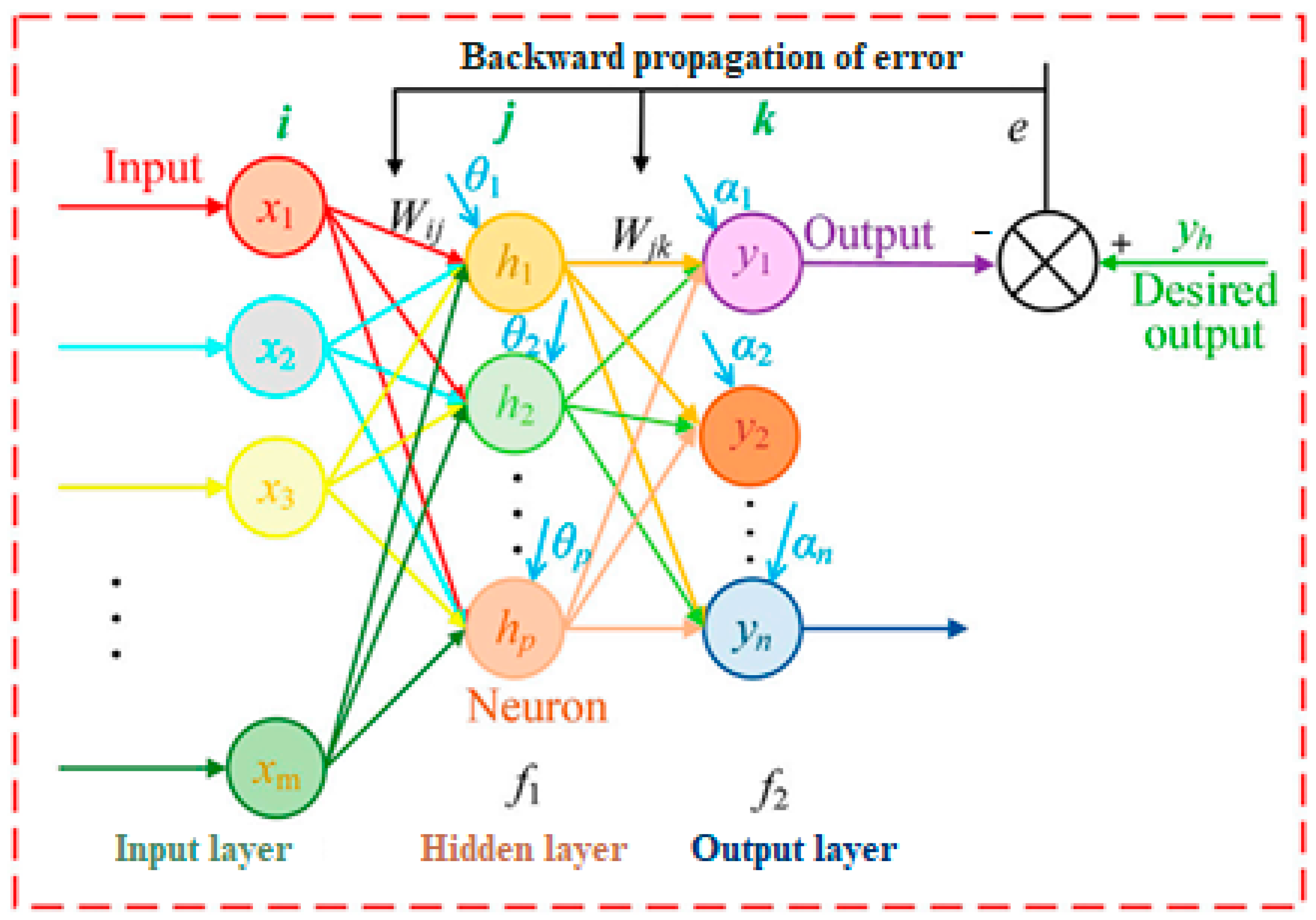
Figure 1 depicts the fundamental structure of a BPNN, illustrating its interconnected layers of artificial neurons that process and transmit information during the learning process.

Backpropagation neural networks (BPNNs) represent a powerful class of artificial neural networks renowned for their ability to learn complex, non-linear relationships between input and output data. Their architecture and functionality are key to understanding their learning capabilities.

The network structure is as follows:

• Layered architecture: BPNNs are characterized by a layered architecture, typically consisting of the following layers:

  ➢

  Input layer: this layer receives the initial input data, representing the features or independent variables used for training.

  ➢

  Hidden layers: these intermediate layers, which are present in varying numbers depending on the network complexity, perform the core information processing and feature extraction within the network.

  ➢

  Output layer: the final layer produces the network’s predicted output, corresponding to the target variable or desired outcome.

• Interconnected neuron nodes: Each layer, except the input layer, comprises interconnected neuron nodes. These nodes act as the fundamental processing units of the network, performing calculations to transform received information.

The neuron node functions are as follows:

• Weighted inputs: Each neuron receives input values from other nodes in the preceding layer. These inputs are multiplied by corresponding weights, which act as learnable parameters that determine the influence of each input on the neuron’s output.
• Activation function: The weighted sum of inputs is then processed through a non-linear activation function. This function introduces non-linearity into the network, enabling it to model complex relationships that cannot be captured by linear models.
• Threshold and output: The output of the activation function is further compared to a threshold value. If the result exceeds the threshold, the neuron is considered “activated” and its output is typically set to one. Otherwise, the output remains zero.

Mathematical Representation

Equation (9) [46] can be used to mathematically model the activation of a single neuron node. It typically involves calculating the weighted sum of its inputs [34,39,41], applying the chosen activation function and potentially comparing the result to a threshold. References [34,36,40] provide further details on specific mathematical formulations used in BPNNs.

In essence, BPNNs leverage the interconnected layers and individual processing capabilities of neuron nodes to progressively learn and adapt their internal parameters, enabling them to capture complex non-linear relationships within data. This learning process, known as backpropagation [40], is further elaborated upon in the following section.

$$Y_j=f\left({{\displaystyle \sum }}_{i=1}^n{w}_i\times X_i-\theta \right)$$

(9)

where $Y_j$ represents the output value of the neuron node, $w_i$ presents the weight associated with input $x_i$, $x_i$ represents the input value to the neuron node, $\theta$ represents the threshold value of the neuron node and $f$ denotes the activation function.

The training process of BPNNs involves two crucial phases: forward propagation and backpropagation of error. These phases work together to iteratively adjust the network’s internal parameters, enabling it to learn and improve its prediction accuracy.

1. Forward propagation comprises the following steps:

• Initialization: The initial step involves assigning random weights to the connections between neurons in different layers. These weights typically fall within a predefined range, such as [−1, 1].
• Input processing: The input layer receives the data from a training sample. This data represents the features or independent variables used for training.
• Layer-wise computation: Information propagates forward through the network layer by layer. At each layer, each neuron receives weighted inputs from the previous layer, applies a non-linear activation function and calculates its output value. This process transforms and transmits the information through the network.
• Output calculation: The final layer processes the information received from the previous layer and generates the network’s final output, representing the predicted value for the given training sample. This completes a single forward propagation cycle [35,40].

2. The backpropagation of error comprises the following steps:

• Error calculation: Once the output is obtained, the network compares it to the desired target value (known from the training data). If there is a difference (error), the backpropagation phase begins.
• Error propagation: The error signal is propagated backward through the network, layer by layer. This involves calculating the contribution of each neuron’s error to the overall network error [43].
• Weight adjustment: Using an optimization algorithm (e.g., gradient descent), the weights connecting the neurons are adjusted in a way that minimizes the overall error. This adjustment process aims to improve the network’s ability to map the input data to the desired output in future training iterations. The weight update rule is given by Equation (10) [33], as follows:

$$W\left(k+1\right)=W\left(k\right)+\alpha D\left(k\right)$$

(10)

where $W\left(k+1\right)$ and $W\left(k\right)$ represent the weight/threshold values in the $(k+1$)th and $k$th iterations, respectively, $\alpha$denotes the learning rate, controlling the magnitude of weight updates and $D\left(k\right)$ represents the negative gradient of the network error with respect to the weights and thresholds, indicating the direction of fastest error reduction.

• Iteration: the training process continues until the network’s output error reaches a predefined threshold or a specified number of iterations is completed.

The forward and backpropagation phases continue iteratively through the entire training dataset. With each iteration, the network progressively adjusts its internal weights, enabling it to learn and refine its ability to map input patterns to the desired outputs. This iterative process ultimately leads to the network’s convergence and improved prediction accuracy [36,43].

2.2. Quality of Model

A well-performing model can provide valuable insights and predictions, while a poor-quality model can lead to misleading results and wasted resources. This section highlights the basic testing metrics for the evaluation of the model.

2.2.1. Correlation Coefficient

The correlation coefficient (r) is a statistical measure that indicates the strength and direction of a linear relationship between two variables. The value of r ranges from −1 to 1. Equation (11) represents the correlation coefficient [25,26,30,34,40], as follows:

$$r=\frac{\sum \left(\mathrm{x} -\overline{\mathrm{x}}\right)\left(\mathrm{y} -\overline{\mathrm{y}}\right)}{\sqrt{\sum {\left(\mathrm{x} -\overline{\mathrm{x}}\right)}^2\sum {\left(\mathrm{y} -\overline{y}\right)}^2}}$$

(11)

where $r$ is the correlation coefficient, $x$ represents the values of one variable, $y$ represents the values of the second variable, $\overline{x}$ represents the mean value of variable $x$ and $\overline{y}$ represents the mean value of variable $y$.

The interpretation is as follows:

• $r$ = 0 indicates that there is no linear relationship between the variables.
• $r$ = 1 indicates that there is a strong positive linear relationship between the variables.
• $r$= −1 indicates that there is a strong negative linear relationship between the variables.

2.2.2. Coefficient of Determination

The quality of the model for a given dataset of observation can be determined using the coefficient of determination, R², which is represented by Equation (12), as follows:

$$R^2={\left[Cor\left(Y,\widehat{Y}\right)\right]}^2=1-\frac{\sum {\left(y_i-{\widehat{y}}_i\right)}^2}{\sum {\left(y_i-{\overline{y}}_i\right)}^2}$$

(12)

where $Cor\left(Y,\widehat{Y}\right)$ is the correlation coefficient, $\sum {\left(y_i-{\widehat{y}}_i\right)}^{2 }$ is the sum of squared errors (SSE) and $\sum {\left(y_i-{\overline{y}}_i\right)}^2$ is the total sum of squares (SST).

The value of R² is between zero and one. However, a high value of R² does not necessarily mean that the model fits the data well. Thus, a more detailed analysis is needed to ensure that the model can be used to describe the observed data and to predict another dataset [27,30].

The coefficient of determination has a tendency to increase with the number of independent variables in the regression model, although these added variables do not carry any new information about the dependent variable. To prevent this artificial increase, refs. [46,47] proposed an adjusted coefficient of determination, which corrected the estimated inflation of the original coefficient of determination and is calculated according to Equation (13), as follows:

$$R_{adj}^2=1-1\left(1-R^2\right)\frac{n-1}{n-p-1}$$

(13)

where $n$ is the number of observations in the dataset and $p$ is the number of variables in the model. $R_{adj}^2$ can be less than zero. However, there are a large number of procedures for adjusting the coefficient of determination, intended for various types of generalization of the prediction quality.

2.2.3. The Root Mean Square Error

The root mean square error model is another model with parameters used to measure the quality of the model. It specifies the variance data around the model. The RMSE for the simple linear model is as follows (Equation (14)) [6,27]:

$$RMSE=\sqrt{\frac{\sum {\left(y_i-{\widehat{y}}_i\right)}^2}{n}}$$

(14)

And, for multiple linear regression, it is as follows (Equation (15)):

$$RMSE=\sqrt{\frac{\sum {\left(y_i-{\widehat{y}}_i\right)}^2}{n-k}}$$

(15)

where n is the number of data points, $y_i$ is the actual value for the i-th data point, ${\hat{y}}_i$ is the predicted value for the i-th data point using the linear model and k is the number of the parameter estimated, including the constant.

3. Methodology

Accurately predicting lighting energy consumption in buildings is a critical cornerstone for effective energy management and achieving sustainability goals. This paper presents a comparative analysis of two prominent prediction methods: polynomial regression and artificial neural networks. We establish a comprehensive methodology for the implementation and evaluation of these approaches, subsequently demonstrating its efficacy through its application to a real-world building energy consumption dataset.

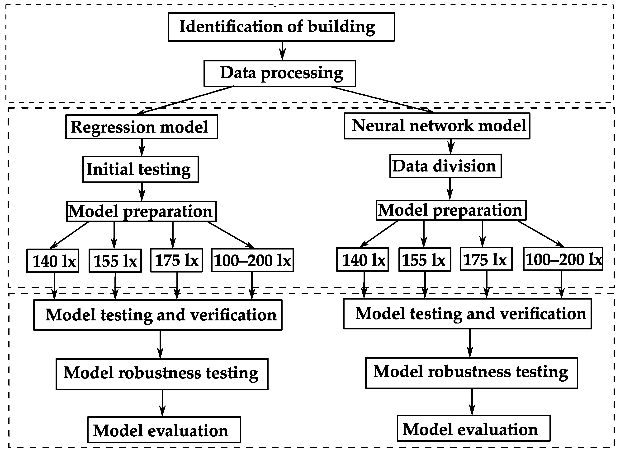
The underlying methodology of this approach is based on a set of well-defined steps, as illustrated in the flowchart presented in Figure 2.

Prior to the development of predictive models, it is of the utmost importance to identify the target building, ascertain its relevant parameters and secure the data necessary for model construction. The subsequent step involves the preprocessing of the data, which encompasses the cleaning, manipulation and imputation of missing values, and their transformation into a suitable format compatible with the chosen predictive models. The subsequent steps are conducted in parallel, employing two distinct approaches.

In the context of regression analysis, preliminary tests are conducted with the objective of determining the most suitable regression variant for the specific application. Following the evaluation of fundamental metrics, the development of a predictive model is undertaken. This article examines the evaluation of various illumination levels (140, 155 and 175 lx and an interval of 100–200 lx). Once each predictive method has been developed, the accuracy of each model is verified. Subsequently, the robustness of the algorithm is tested to ascertain its behavior based on diverse input values. Finally, the accuracy results for each algorithm are evaluated and compared.

In the case of a neural network, the procedure is analogous, but due to the nature of this method, the data is initially divided into three groups: training, validation and testing sets. Each neural network is trained and tested for specific illumination values using the aforementioned datasets. Similarly to the regression approach, subsequent testing is conducted using an independent dataset, followed by robustness testing of the algorithms for specific input values. Finally, the resulting errors and metrics are determined, which serve as indicators of the model’s overall quality and, consequently, its predictive performance.

4. Prediction Model

This paper presents a comparative analysis of two distinct modeling approaches for prediction: polynomial regression and artificial neural networks. The first section of the study focuses on the application and accuracy verification of a model based on polynomial regression. The second section explores the application of ANNs and assesses their predictive accuracy. Finally, a comprehensive comparison of the two models is provided (

Table 3. Comparison of polynomial regression and artificial neural network models.

Feature	Polynomial Regression Model	Artificial Neural Network Model
Model description	Uses polynomial function to approximate relationships between input and target variables. Degree of the polynomial determines complexity and ability to capture non-linearity.	Inspired by the human brain and uses interconnected layers of artificial neurons. Each neuron performs a non-linear transformation, allowing the model to learn complex patterns.
Model training	Not applicable—model fits data directly based on chosen polynomial degree.	Requires training data and an iterative process called backpropagation to adjust weights of connections between neurons.
Accuracy assessment	Evaluated using statistical measures like R-squared (R2), root mean square error (RMSE) and correlation coefficient (r).	Evaluated using similar statistical measures (R2, RMSE and r).
Advantages	Simple to understand and implement; Relatively fast to train and use; Interpretable: coefficients of the polynomial function reveal variable importance.	Models complex non-linear relationships effectively; Handles high-dimensional data well; Generalizes well to unseen data (within the range it was trained on),
Limitations	Limited to capturing relationships expressible by chosen polynomial function; Prone to overfitting, especially with high-dimensional data and high polynomial degrees; Less accurate for complex non-linear relationships.	Computationally expensive to train, especially for large datasets or complex architectures; Prone to overfitting if not properly regularized; Difficult to interpret: “black box” nature makes it hard to understand how the model arrives at its predictions.
Use	Suitable for linear or slightly non-linear relationships; Good for initial exploration and understanding data; Useful when interpretability is crucial.	Ideal for complex non-linear relationships; Effective for high-dimensional data; Preferred when generalization to unseen data is important.
Additional considerations	Choosing the right polynomial degree is crucial for accuracy and avoiding overfitting; Feature scaling might be necessary for some algorithms.	Requires careful selection of network architecture, activation functions and learning parameters; Regularization techniques are often needed to prevent overfitting.

) in terms of their accuracy and suitability for different scenarios.

4.1. The Building Description and Dataset Acquisition

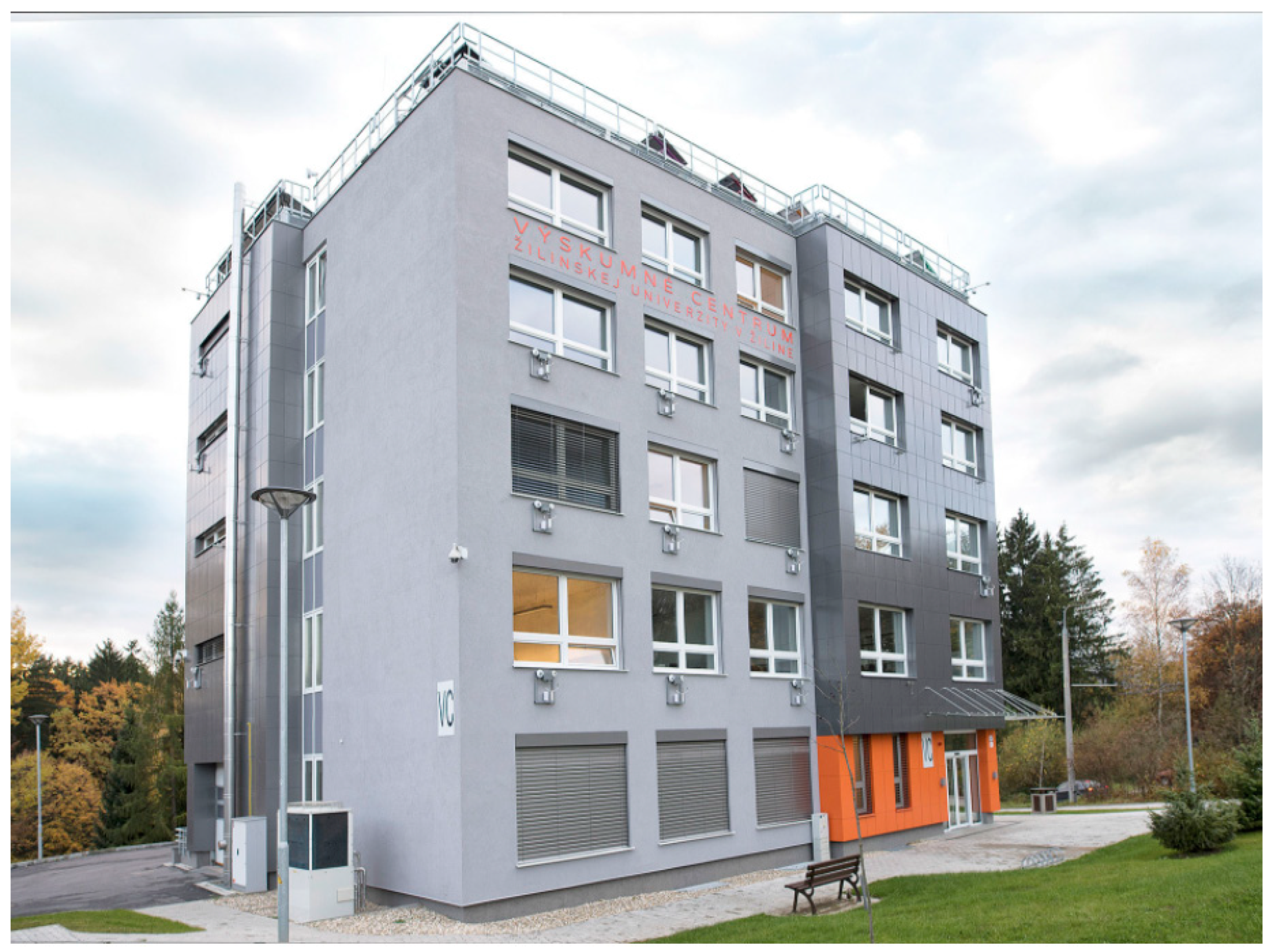
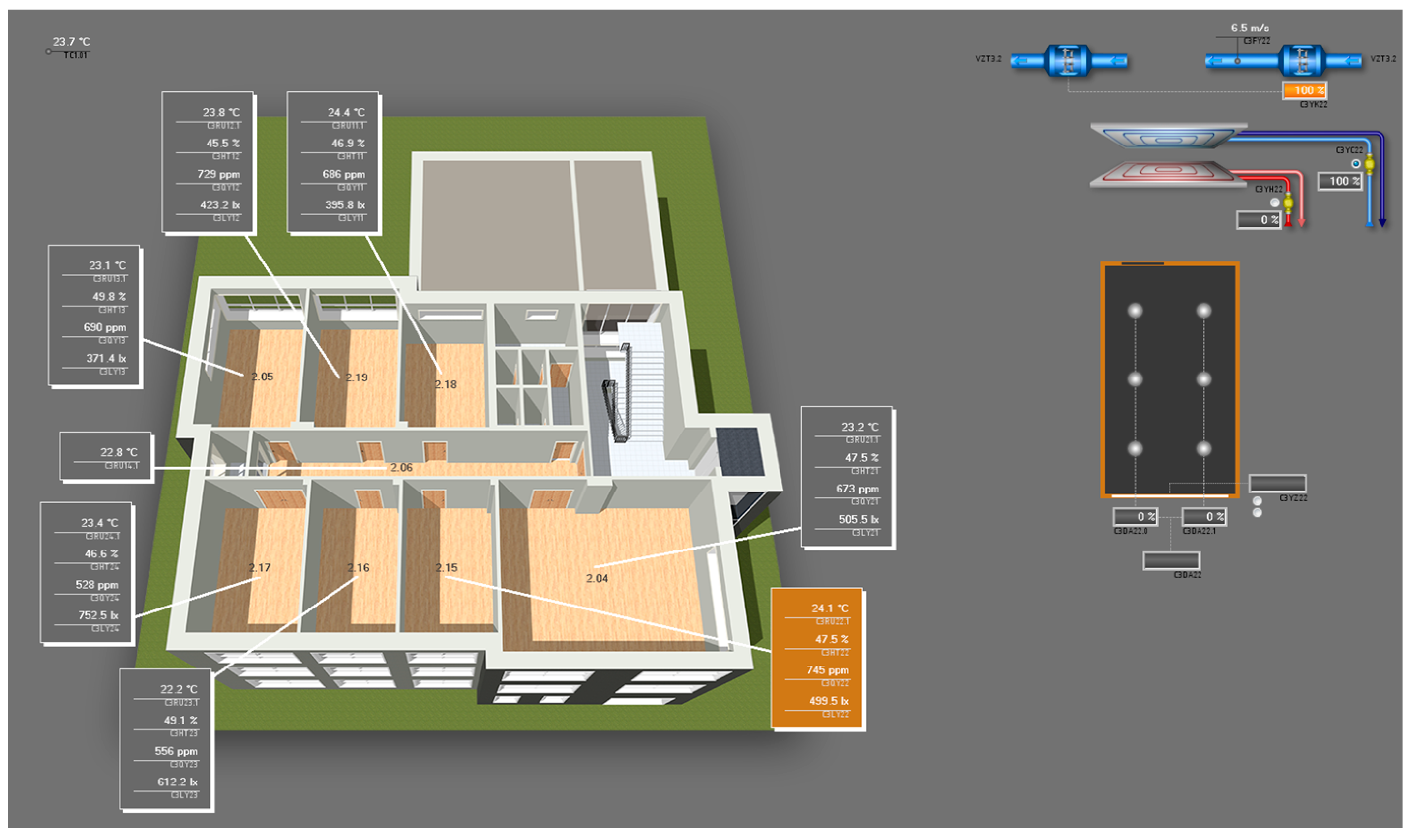
The Research Centre of the University of Zilina was chosen for this study. The Research Centre is a five-floor building. On the ground floor and 1st floor are the laboratories and on the other floors are the office spaces. The whole building is designed as an intelligent building. Because the building was designed for the experimental development of intelligent buildings and systems, in each room, a sensor which collects data on the internal thermal comfort, lighting, etc. was installed. The control system allows occupants to change individual parameters for each room separately. On the exterior of the building, there is a built-in weather station at each window, which collects data on external conditions. This building design is very suitable for the experimental testing of different systems as the building and its control system provide a large amount of measured data. The measured data are collected in 5 min intervals. Figure 3 shows the building of The Research Centre and Figure 4 shows the control system of the building, where it is possible to see, in real-time, all of the above-mentioned data. The building is equipped with manually operated shutters on both the east and west sides of the windows. These shutters are primarily utilized by employees to provide glare protection from the sun and excessive heat, particularly during the morning hours on the east side and the afternoon hours on the west side.

The application and verification for other spaces will be described in the next section. In addition to the sensors, which are installed in the system, another sensor was added. More specifically, it is a lux meter, which was used for additional measurements of the light intensity in the working plane of the space (desktop). For this measurement, a certified digital lux meter DT-8809A was used. The main reason for the installation of the lux meter was the determination of the light intensity at the level of 0.8 m, because the light sensor for the control system is located on the ceiling.

For the study, only data directly related to the lighting system were used. The created dataset contained data on the consumption of lighting and external intensity of lighting. The consumption of electrical energy was expressed in the form of an electric current. It is possible to calculate the total consumption as well as other parameters from the electric current using the basic electric formulas (the parameters required for conversion to consumption are as follows: V = 230 V, PF = 0.9). The external intensity was obtained in a meter station located on the west side of the building because of the orientation of the building (location of testing space). The data consisted of 5 min measurement intervals. These data were subsequently processed and transformed into the data necessary for polynomial regression. The data were adjusted, as it was necessary to detect and supplement the missing data at some intervals or remove incorrectly measured data. For example, it was edited the data regarding the external intensity was edited, since, at night, while it was dark outdoors, the sensor still measured a value of about 3000 lx; therefore, during the night, the data were adjusted to a value of 0 lx. These data were used to predict the lighting consumption for spaces of different set lighting intensities. Similarly, data were obtained and modified which were used to verify the suitability of the proposed prediction model.

In the spaces, the lighting intensity was set using the central control system. After this setting, the lighting was put under autonomous control and the occupants of the building could not change the set intensity. The experimental measurements were collected in a 24/7 mode, in order to determine the overall function based on the polynomial regression analysis for the whole lighting range (from complete darkness to maximum daylight). Daylight is a combination of light from direct sunlight as well as diffused light from the sky. At night, regulation was also necessary because the installed lighting was oversized. In this case, total power of lighting was not used; instead, only an aliquot part was used, according to the set intensity. 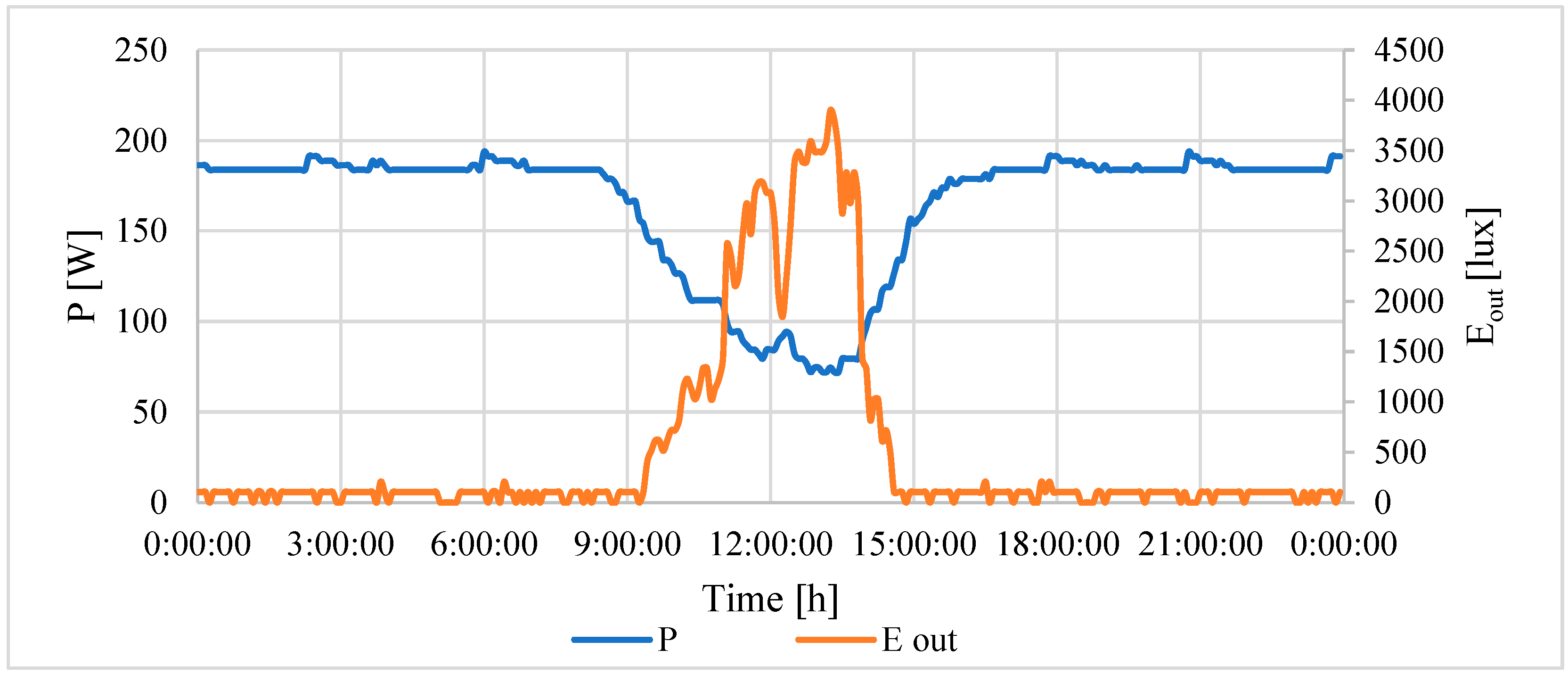The following Figure 5 shows the curve of consumption and intensity for the selected day. The blue curve represents an electric current. The orange curve represents the external intensity lighting. In this image, the relationship between the external intensity and the current taken is obvious.

4.2. Prediction Model Utilizing Regression Analysis

Before undertaking the prediction, it was necessary to find the most suitable data model to best correspond to the measured data. As part of the preparation, seven different possibilities for statistical analysis were realized.

In each case, the suitability of the possible prediction function was tested by comparing the correlation coefficients. The following

Table 4. Correlation coefficients of different types of regression.

	Correlation Coefficient			R2
	140 lx	155 lx	175 lx	140 lx	155 lx	175 lx
Linear curve	0.926	0.931	0.925	0.857	0.866	0.856
Polynomial 2nd degree curve	0.961	0.971	0.959	0.924	0.943	0.920
Polynomial 3rd degree curve	0.965	0.973	0.966	0.931	0.947	0.934
Polynomial 4th degree curve	0.952	0.971	0.961	0.907	0.943	0.924
Hyperbolic curve	0.252	0.919	0.481	0.063	0.844	0.232
Logarithmic curve	0.669	0.843	0.755	0.448	0.712	0.571
Exponential curve	0.953	0.951	0.946	0.910	0.906	0.896
Power curve	0.669	0.918	0.755	0.448	0.844	0.571

shows the results for the individual prediction functions for the lighting values 140, 155 and 175 lx (control system sensor). These three values of 140, 155 and 175 lx are the thresholds for when the lighting systems start to operate. Based on the results of the comparison, a polynomial regression function was determined to be the most suitable solution. The next section provides a detailed description of the determination of the necessary coefficients, as well as its application and verification.

4.2.1. Application of Polynomial Regression to Consumption Prediction

This section describes the application of polynomial regression to the measured dataset. According to the additional surveys, there was no consensus among the occupants on the resulting lighting intensity (each resident had different lighting requirements). In order to be able to reflect the wellbeing of the occupants of the buildings, three measurements were made, as well as regression analysis, for the different light intensities. This procedure will make it possible to better predict the resulting lighting consumption, as it is possible to better adapt to the requirements of the occupants, making the resulting prediction more accurate.

In the first step, three levels of illumination were selected to test the suitability and applicability of the polynomial regression analysis. Based on the results, a prediction function was subsequently developed for illumination in the interval of 100–200 lx (from the sensors of the control system). In this interval, all lighting levels obtained from the survey of the building users were included.

The polynomial regression was developed in the program "regression function" in the Excel Data Analysis package [48]. The developed analysis will make it possible to predict the development of consumption based on the independent variable (the external intensity of lighting). Excel was chosen because of its simplicity and widespread distribution throughout the world. This allows easy applicability in practice. The regression analysis in the MS Excel program was based on the method of least squares.

Using Equation (5) and Excel, a regression analysis was made for a lighting value of 175 lx (from the sensor of the control system). At this value of the sensor, the value at the level of 0.8 m was 650 lx (desktop illuminance). This value corresponded to standard EN 12464-1 [49]. The resulting function for a prediction is as follows:

$$P=189.98+\left(-0.10269\right)\times E_{out}+\left(3.58\times {10}^{-5}\right)\ast E_{out}^2+\left(-4.6\times {10}^{-9}\right)\times E_{out}^3$$

(16)

The evaluation of the quality of the model is as follows: coefficient R² = 0.9314, correlation coefficient 0.9651 and RMSE = 9.63 W.

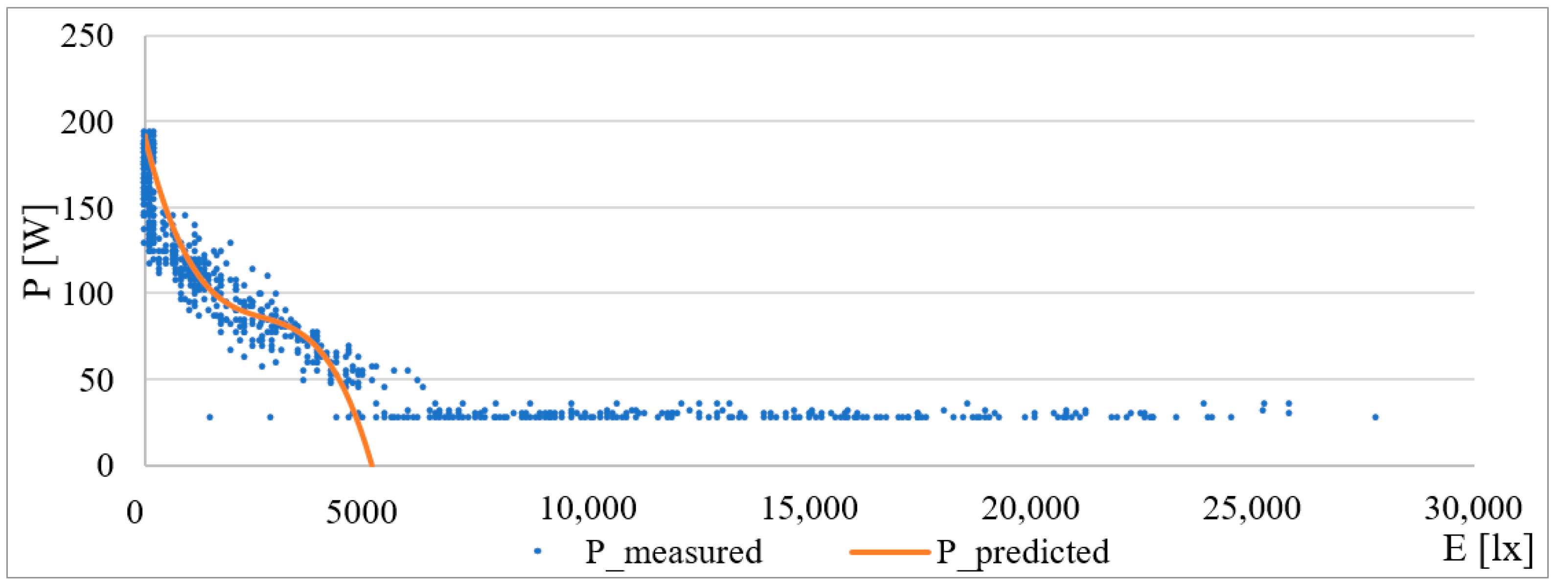
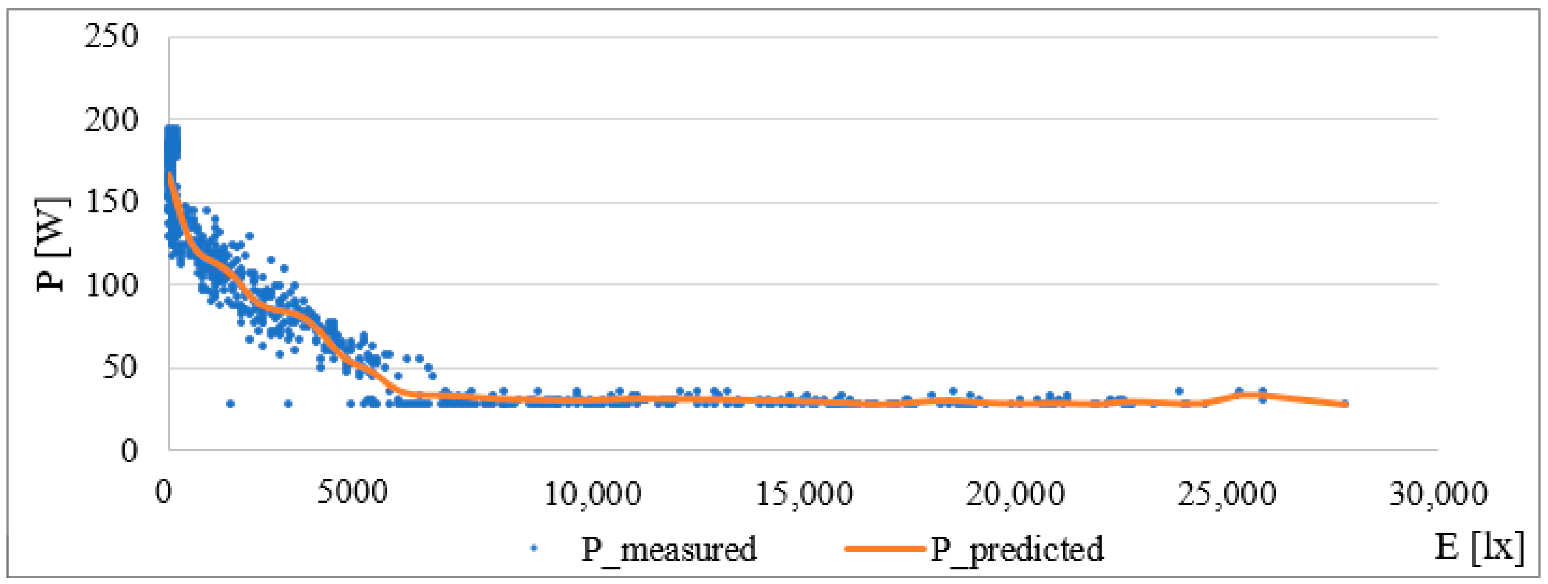
Based on this function, a curve describing the change in consumption according to external lighting was created. The graphic interpretation of the given model is in the following Figure 6. For values larger than approx. 5300 lx (daylight), the curve goes into the negative, which, in practice, means that the lighting has no consumption; it is switched off. In the predicted value, this negative state can be eliminated by a simple condition. Coefficient β₀ = 189.98 corresponds approximately to the consumption of lighting without daylight.

Another step to verify the suitability of the model on the dataset was to test the null hypothesis at the selected significance level α. In this model, a significance level of 0.05 was selected. For the test of the null hypothesis, an F-test was used. For the selected model, the calculated value (Significance_F) was 7.0273 × 10⁻¹⁶⁵ < 0.05. According to this test, the null hypothesis was rejected and it can be said that the model was chosen correctly.

The next step was the determination of the statistical significance of the calculated correlation coefficients. The null hypothesis for this test states that the coefficients are insignificant, and the alternative hypothesis states the opposite. The verification of this hypothesis was performed using a p-value for individual coefficients.

The following

Table 5. Coefficients and the null hypothesis test 175 lx.

	Coefficients	p-Value	α	Results
β0	189.98	0	0.05	0 < 0.05
β1	−0.10269	5.32 × 10−53	0.05	5.32 × 10−53 < 0.05
β2	3.58 × 10−5	3.91 × 10−16	0.05	3.91 × 10−16 < 0.05
β3	−4.6 × 10−9	4.99 × 10−8	0.05	4.99 × 10−8 < 0.05

contains the coefficients, their p-values and the test of the null hypothesis. The table shows that all coefficients were statistically significant, and the null hypothesis was rejected.

• 155 lx

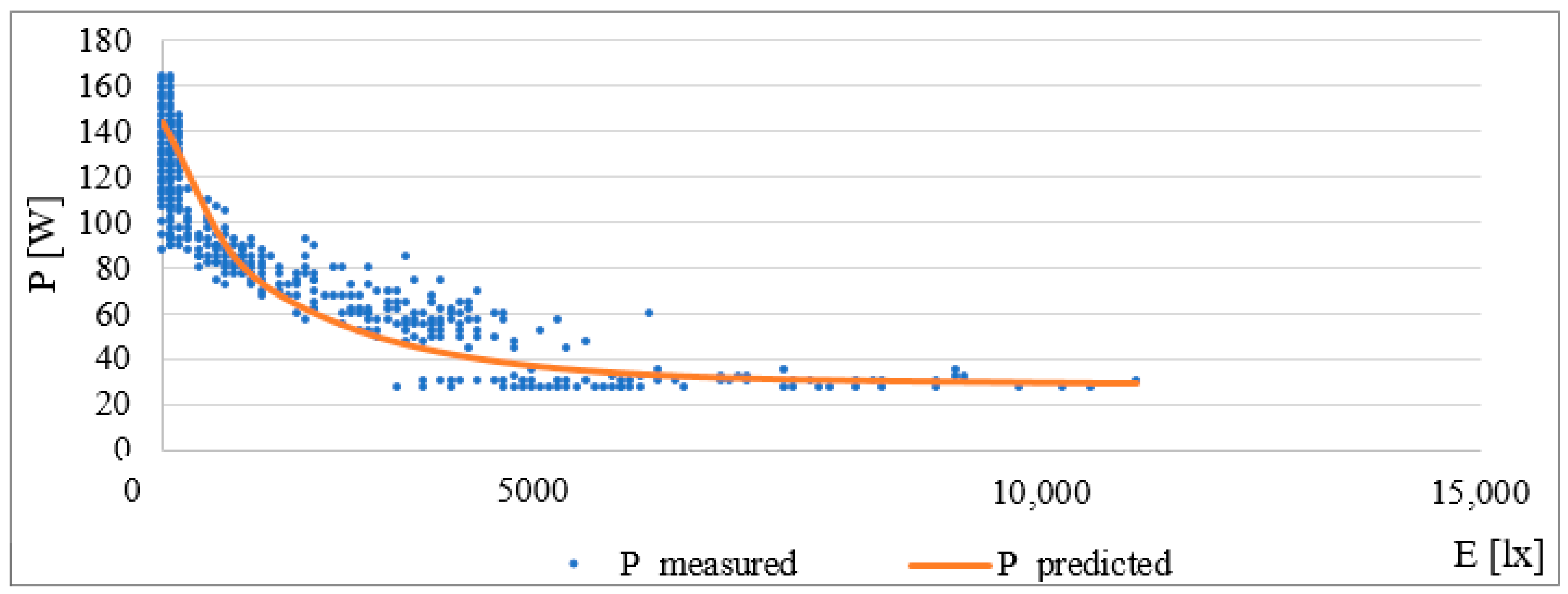
As in the previous case with Equation (5), a regression analysis was carried out. In this case, the value at the level of 0.8 m was 520 lx (desktop illuminance). This value corresponded to standard EN 12464-1. The prediction function for this intensity is as follows:

$$P=156.51+\left(-0.08233\right)\times E_{out}+\left(2.4\times {10}^{-5}\right)\ast E_{out}^2+\left(-2.5\times {10}^{-9}\right)\times E_{out}^3$$

(17)

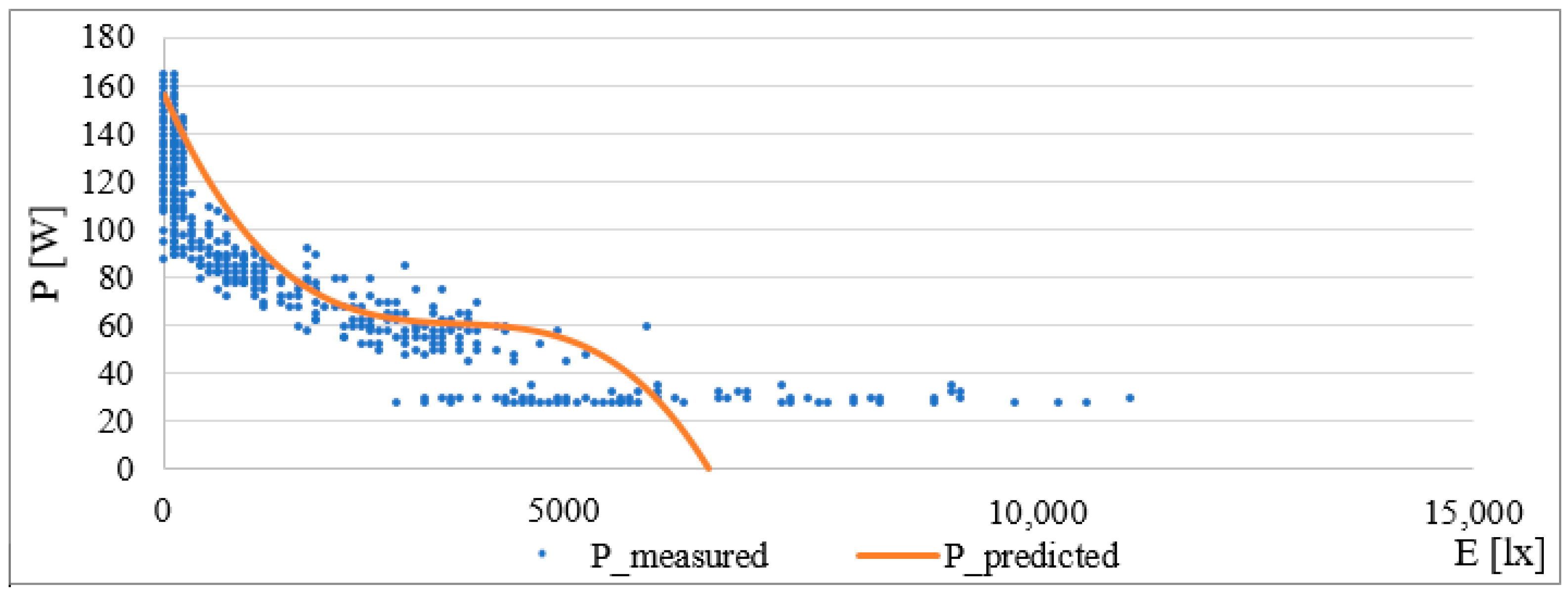
The evaluation of the quality of the model is as follows: the coefficient of determination, R², = 0.9334, the correlation coefficient is 0.966 and RMSE = 9.81 W. The correlation coefficient with a value of 0.966 clearly shows the correlation and the strong dependence between the variables (in this case, the external intensity and the measured current). The graphical interpretation is the normal range of external intensity, and is shown in Figure 7.

The verification of the null hypothesis was carried out, as in the previous part, according to the F test. The calculated value (Significance_F) was 5.8625 ×∙10⁻¹⁶⁷ < 0.05, so the null hypothesis was rejected and the developed model was proven to have been created correctly. The verification of the statistical significance of the coefficient β is shown in the following

Table 6. Coefficients and the null hypothesis test for 155 lx.

	Coefficients	p-Value	α	Results
β0	156.51	0	0.05	0 < 0.05
β1	−0.08233	3.09 × 10−56	0.05	3.09 × 10−56 < 0.05
β2	2.4 × 10−5	5.16 × 10−22	0.05	5.16 × 10−22 < 0.05
β3	−2.5 × 10−9	2.66 × 10−13	0.05	2.66 × 10−13 < 0.05

.

On the basis of the result, the null hypothesis was rejected and the alternative hypothesis was accepted, so the calculated coefficients were statistically significant.

• 140 lx

As in the previous cases, regression analysis was performed using the MS Excel program. Compared to the previous case, the difference is that the measured value at 0.8 m was 450 lx (desktop illuminance). This value no longer corresponded directly to the EN 12464-1 standard, but, according to the survey of the occupants, it was sufficient to perform work tasks.

The final prediction function is as follows:

$$P=145.806+\left(-0.06591\right)\times E_{out}+\left(1.252\times {10}^{-5}\right)\times E_{out}^2+\left(-7.9\times {10}^{-10}\right)\times E_{out}^3$$

(18)

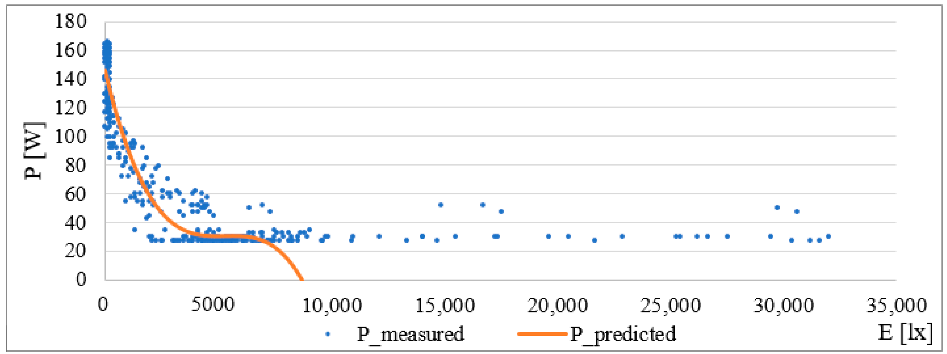
The evaluation of the quality of the model is as follows: R² = 0.9472, correlation coefficient = 0.9732 and RMSE = 9.48 W. As in previous cases, there was a strong degree of dependence between variables. The following Figure 8 shows a graphical representation of the prediction function.

The verification of the null hypothesis was carried out, as in the previous part, according to the F test. The calculated value (Significance_F) was 6.9 × 10⁻¹⁸¹ < 0.05, so the null hypothesis was rejected and the developed model was proven to have been created correctly. The verification of the statistical significance of the coefficient β is shown in the following

Table 7. Coefficients and the null hypothesis test for 140 lx.

	Coefficients	p-Value	α	Results
β0	145.806	5.9 × 10−283	0.05	5.9 × 10−283 < 0.05
β1	−0.06591	1.93 × 10−47	0.05	1.93 × 10−47 < 0.05
β2	0.00001252	2.17 × 10−14	0.05	1.93 × 10−47 < 0.05
β3	−7.9 × 10−10	1.43 × 10−6	0.05	21.43 × 10−6 < 0.05

.

On the basis of the result, the null hypothesis was rejected and the alternative hypothesis was accepted, so the calculated coefficients were statistically significant.

4.2.2. Accuracy Verification and Comparison of Individual Models

This part describes the verification of the correctness of the created model. This verification is based on the comparison of the measured data and the data which was calculated by the prediction function. Verification was performed for each setting of light intensity (140, 155 and 175 lx). Based on the measured data, it was found that the lighting had a stand-by consumption of about 31 W, even when the light was off. During the verification, this state was achieved by adjusting the value on the basis of the conditions, in order to be able to compare the courses of measured and calculated values. The condition was as follows: if the calculated value was less than 31 W, all smaller values were set to this value. In general, a condition would be set to the value zero, as the results would then be negative, which, in terms of real-world lighting, does not make sense.

• Verification for 140 lx

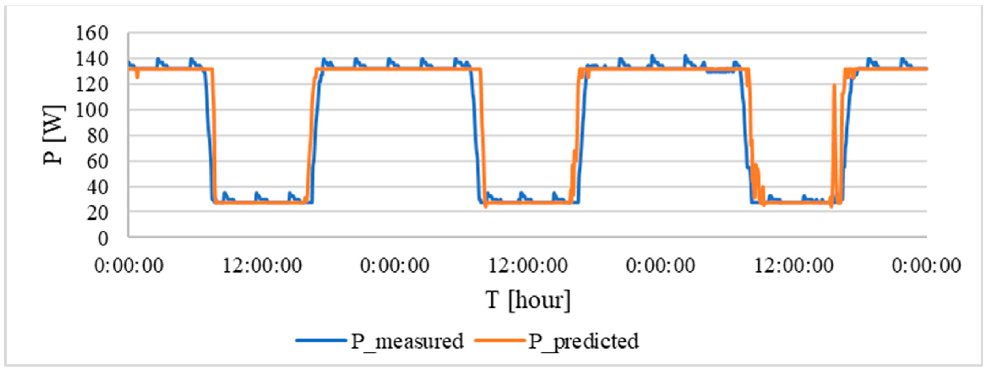
For verification, measurements of intensity in a selected area of the building over a period of several days were made. In the following Figure 9, the curve of the measured value of the electric current and the calculated value according to the regression analysis for the 140 lx are shown.

The blue curve represents the measured value of the current taken for the set interior intensity of 140 lx. The orange curve is calculated according to the prediction function. In the event of a blue curve, there were some peaks at night and during the day, which were caused by a measurement error. In this case, the coefficient β₀ was determined to be the value of 131 W at the base of the measurement, which corresponds to the illumination consumption while maintaining an intensity of 140 lx in the internal space. From the given image, it is possible to determine that the calculated values correspond to the measured data. The total error is shown in

Table 8. Errors of polynomial regression models.

	RMSE [W]	Error [%]	r [−]	R2 [−]
140 lx	16.731	10	0.916	0.839
155 lx	17.720	9	0.931	0.866
175 lx	9.154	5	0.945	0.893

.

• Verification for 155 lx

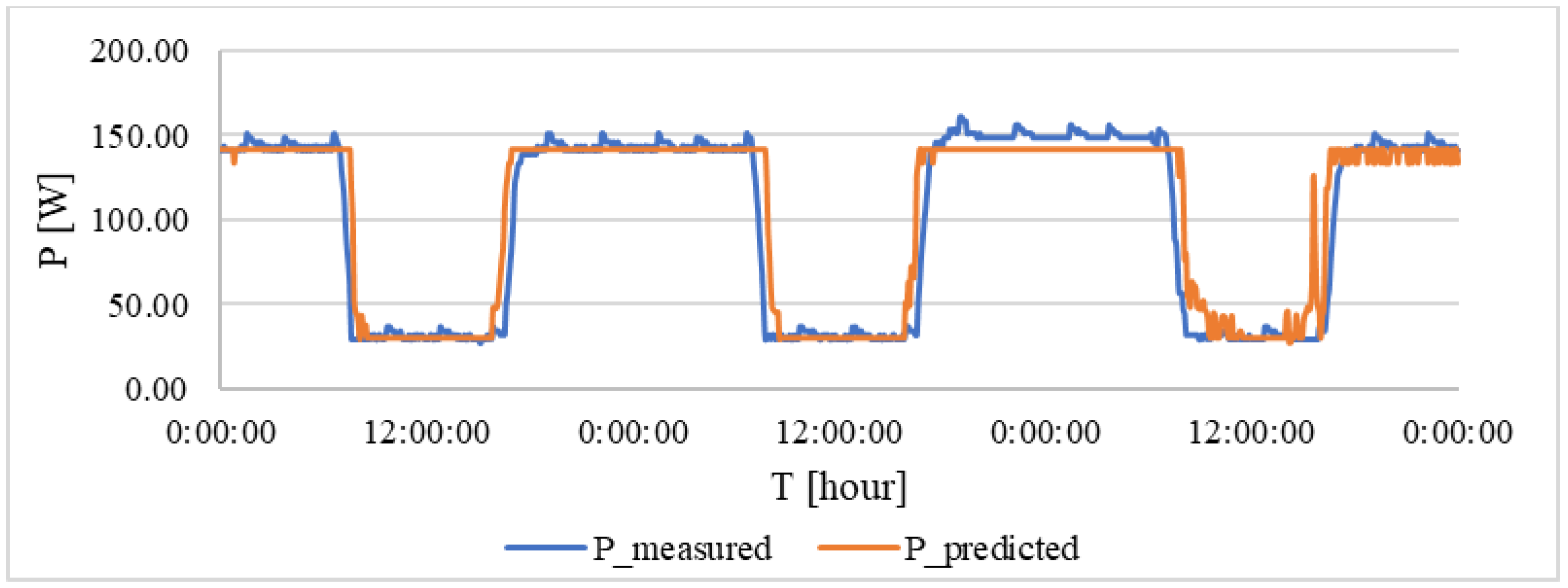
The verification was carried out in a similar way to previous cases. The following Figure 10 is a comparison between the measured and predicted data.

As in the previous case, the coefficient β₀ was determined on the basis of the consumption required to maintain the required lighting level, the value of which is 141 W. The RSME is shown in Table 8. Also, it is possible to notice fluctuations on the third day of verification. This fluctuation was caused by the insufficient intensity of external lighting or by the fact that the illumination value was within the limits necessary to achieve the required internal illumination intensity.

• Verification for 175 lx

The verification was carried out in a similar way to the previous cases. The following Figure 11 is a comparison between the measured and predicted data.

The coefficient β₀ was determined to be 163 W. The resulting RMSE is shown in Table 8.

4.2.3. Comparing the Accuracy of Individual Models for Light Intensity

To evaluate the accuracy of the model, RSME error and average relative error were calculated for each level of light intensity. The following Table 8 compares the errors for the mentioned lighting levels.

At 140 lx, the RMSE was 16.73 W and the relative error was 10%. For 155 lx, the resulting RSME was 17.72 W and the relative error was 9%. For 175 lx, the RMSE was 9.154 W and the relative error was 5%.

The best values of the RMSE and the average relative error were achieved for a lighting value of 175 lx. Since, in this case, the value is higher, the lighting is switched on earlier and, thus, it is less sensitive to fluctuations in the external intensity.

On the basis of these data and results, it can be said that these models provide a relatively accurate prediction of consumption. The resulting error is most influenced by external light conditions and measurement accuracy.

On the basis of developed prediction models, there is a strong dependence between external intensity (daylight) and electric current. This is supported by the obtained high R² values and correlation coefficients (>93%). The final error is approximately 9.315 W, which can be considered satisfactory for the accuracy of the measurement.

From the graphical representation of the individual curves of the current, which depend on the external intensity, the similarity between all the evaluations of the lighting levels is obvious. From these dependencies, it follows that, the lower the internal value is set, the bigger the range of light energy that daylight is able to deliver. The values of the coefficient β₀ correspond approximately to the value of the current consumption without daylight. The values of the other coefficients are also the same. This coefficient can be determined either theoretically, according to the power of the lamps, or by measuring lighting consumption.

4.3. Prediction Model Utilizing Artificial Neural Networks

This section details the development and implementation of a prediction model based on artificial neural networks. The training, validation and testing processes were conducted within the MATLAB R2020b software environment. To guarantee consistency and facilitate the optimization of individual pre-processing steps, identical input data were employed for the training, validation and testing of the network architecture.

Developing a prediction model with Artificial Neural Networks

This section outlines the systematic approach to constructing an accurate consumption model using artificial neural networks. The process involves three crucial stages: data pre-processing, neural network modelling and rigorous model evaluation.

1. Data pre-processing

Data analysis: The first step involves a comprehensive examination of the consumption behavior data, which typically includes energy consumption. This granular examination aims to identify potential patterns, trends and variations in consumption behavior over different conditioning, revealing the temporal dynamics of consumption habits.

Data cleansing: To ensure the integrity and reliability of the data for subsequent modelling, the dataset is meticulously cleaned. This step involves identifying and eliminating any missing values or inconsistencies that may have been introduced during data collection or processing.

2. Neural network modelling

Data import: The pre-processed data are seamlessly imported into the MATLAB environment. This robust numerical computing platform provides an ideal environment for building and training the neural network model.

Data partitioning: The dataset is strategically divided into three distinct subsets: training data (70%), validation data (15%) and test data (15%). This partitioning approach ensures that the model is adequately trained on a representative portion of the data (70%), rigorously tested on unseen data (15%) to assess its generalizability and thoroughly validated on another unseen dataset (15%) to evaluate its performance.

Neural network architecture design: Carefully designed ANN architecture is constructed to capture the complex relationship between external light intensity and energy consumption. The ANN architecture is designed with careful consideration of the complexity of the data and the desired level of accuracy. This thoughtful design ensures that the model effectively learns the underlying patterns and trends within the data, enabling accurate predictions of energy consumption based on external light intensity.

Building an ANN includes the following steps:

• Training: The ANN is trained using the specified training data. During this process, the network learns the underlying patterns and relationships within the data. The training process involves optimizing the network parameters to minimize the difference between predicted and actual energy consumption.
• Validation: The performance of the trained ANN is evaluated using the validation and test datasets. Evaluation metrics such as RMSE, R² and r are used to assess the model’s ability to accurately predict changing energy consumption for previously unseen data.

3. Model Saving

Parameter saving: Following a satisfactory performance evaluation based on the validation and test data, the parameters that define the trained ANN model are stored. These parameters encapsulate the learned knowledge of the model and allow it to be used for future predictions of energy consumption based on external light intensity.

4.3.1. Application of Neural Network Model to Consumption Prediction

By integrating a dataset into a neural network model, we achieved more accurate predictions of lighting consumption. The model’s ability to learn and adapt to individual occupant requirements will ultimately lead to a more personalized and energy-efficient lighting experience.

• 175 lx

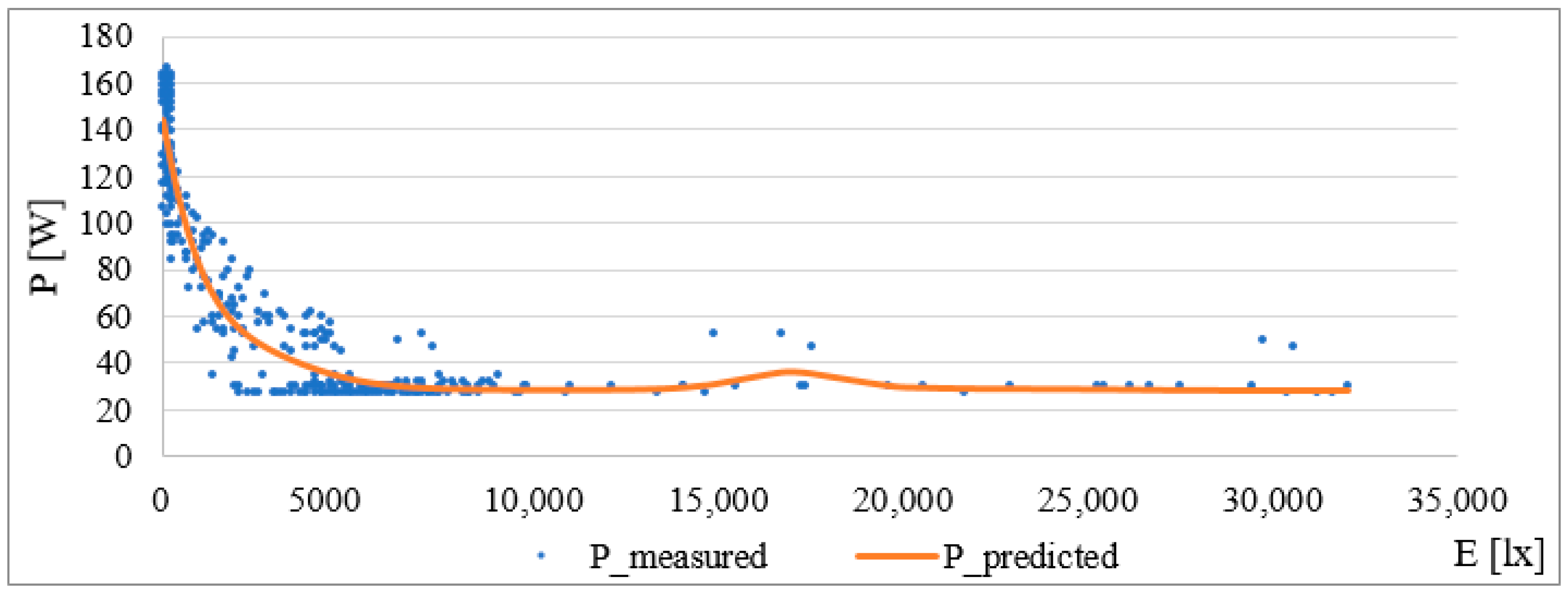
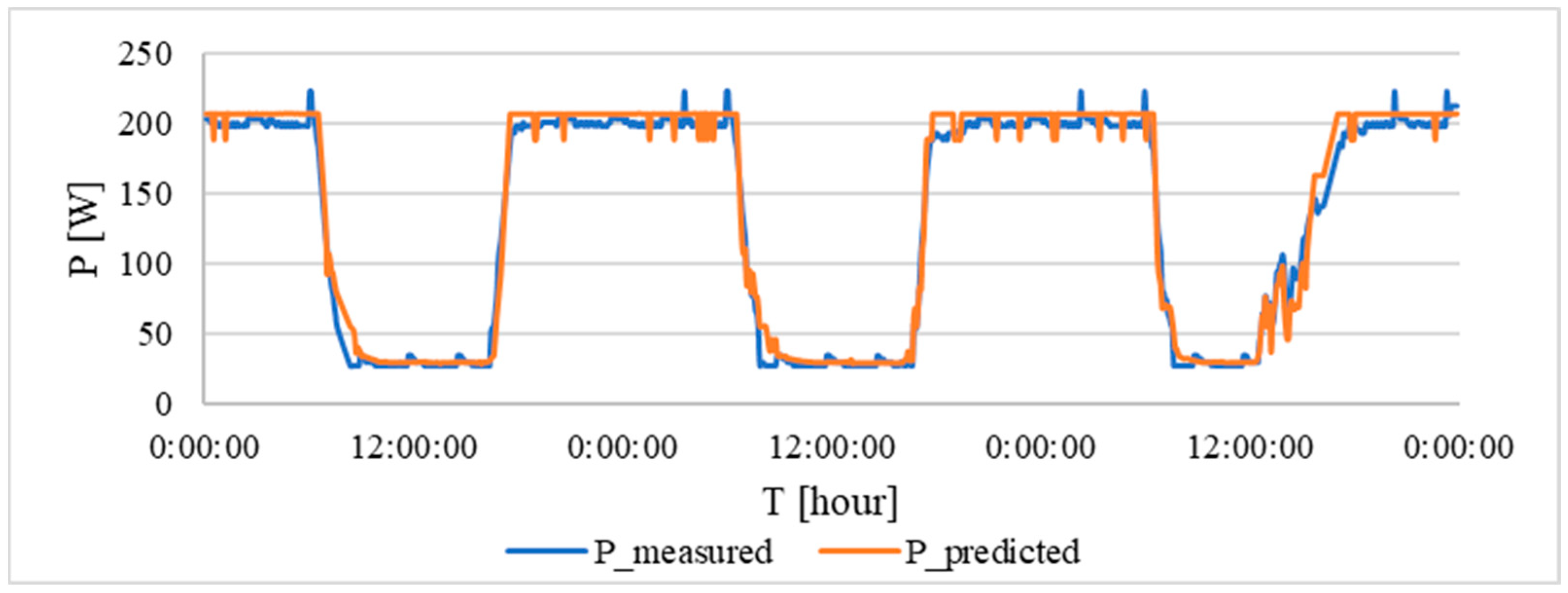
Figure 12 below shows the measured current (blue) and the approximated current obtained using a neural network (orange). There is a high degree of correlation between the two curves. This indicates the excellent accuracy and practical applicability of the neural network model.

The experimental results show that the approximated curve effectively captures the central tendency of the measured data. This indicates that an optimal balance has been achieved between accuracy and the input data used by the network. The resulting approximation matches the measured values, which is reflected in the overall performance and accuracy of the network. Over 100 trials, the RMSE was 3.8 W, the correlation coefficient was 0.987 and the R² coefficient was 0.975. These metrics demonstrate the effectiveness of the chosen approach in approximating the values.

• 155 lx

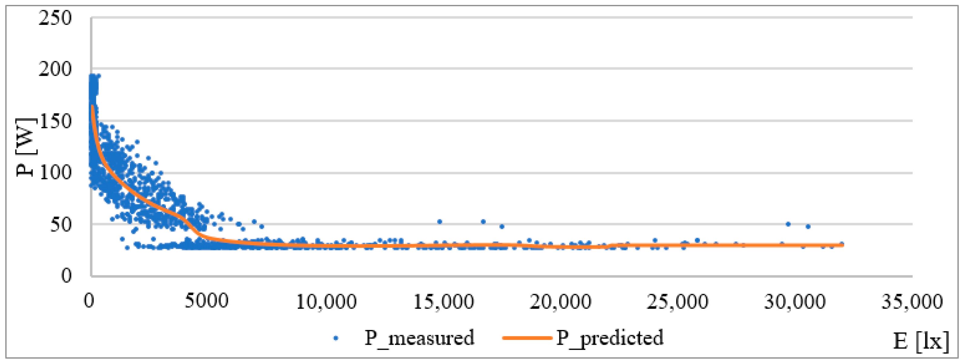
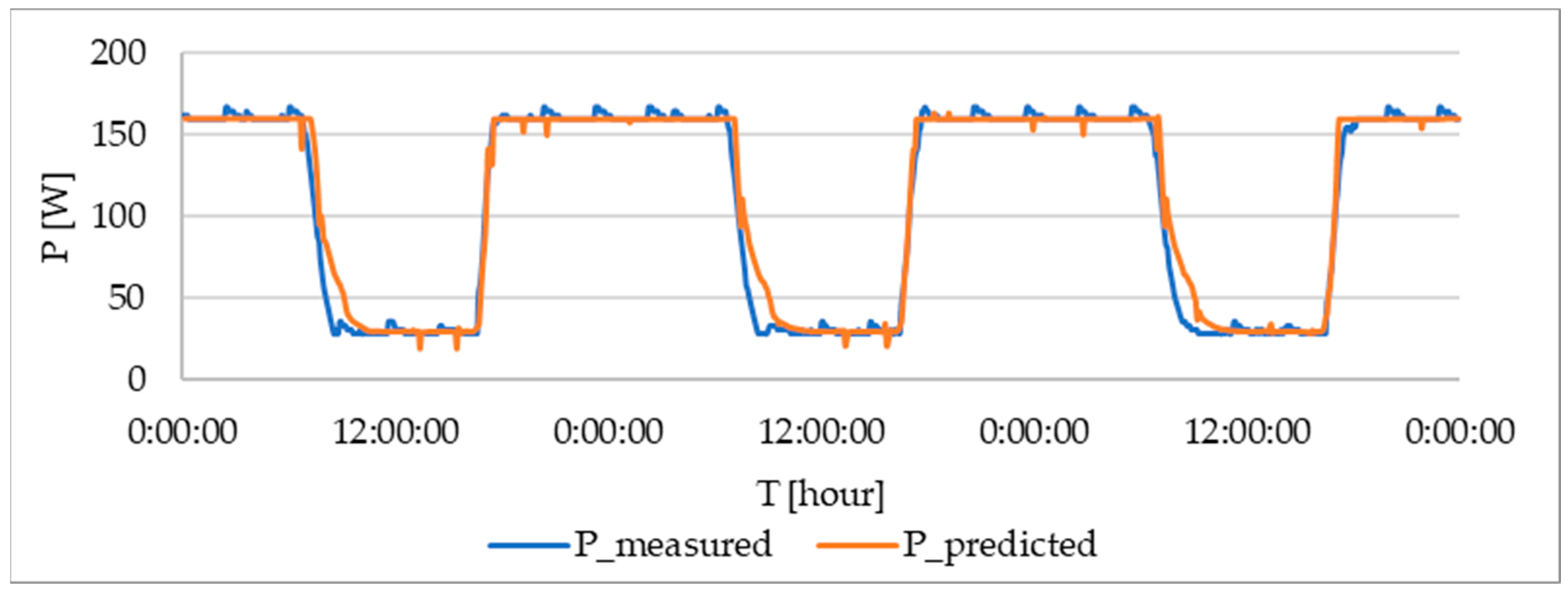
As in the previous experiment, the neural network was trained at 155 lx. Figure 13 shows the response, similar to the previous case. The measured data is represented by the blue curve, while the predicted response from the neural network is shown in orange.

Figure 13 shows that the central tendency of the fit has been again reached. This approach is demanded, as the final curve effectively meets the requirements of the data and achieves the desired level of approximation relative to the input data. Similar to the previous experiment, over 100 simulations were performed, resulting in a RMSE of 4.7 W, a correlation coefficient of 0.982 and an R² coefficient of 0.965. These performance metrics indicate that the artificial neural network, trained on the input data, has a high degree of accuracy when predicting total power consumption.

• 140 lx

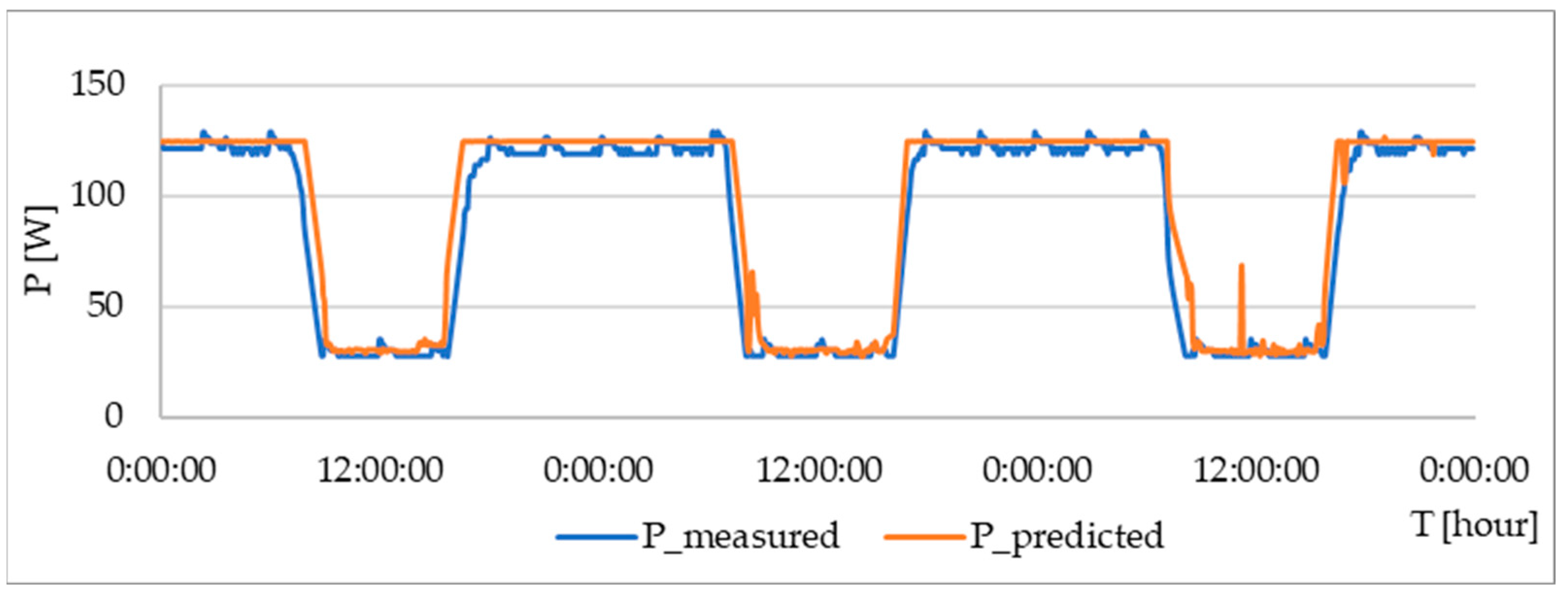
In accordance with the methodology used in the previous experiment, the neural network was trained under a controlled light intensity of 140 lx. Figure 14 shows the resulting transient response, with the measured data represented by the blue curve and the predicted response generated by the neural network represented by the orange curve. This visual comparison allows for a qualitative assessment of the performance of the network in approximating the actual system behavior.

Figure 14 shows that the central tendency of the fit has been reached again. This tendency is necessary to achieve a curve that effectively fits the data and has the desired level of approximation relative to the input data. Consistent with the previous experiment, 100 simulations were performed, yielding a RMSE of 4.2 W, a correlation coefficient of 0.984 and an R² coefficient of 0.970. These performance metrics demonstrate the strong ability of the artificial neural network, trained on the input data, to predict total power consumption with high accuracy.

4.3.2. Accuracy Verification and Comparison of Individual Models

To assess the generalizability of the model, its accuracy was evaluated using independent measurement data. This approach reflects the testing and verification procedures commonly used for prediction models. Specifically, the performance of the network was evaluated at each previously trained light level. The following sections provide a detailed description of the verification results obtained for each individual intensity level.

• 140 lx

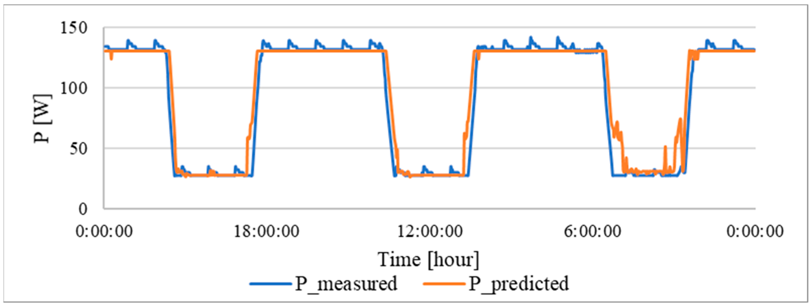
To verify the model’s accuracy under real-world conditions, the intensity of electric current in a building was measured over several days. Figure 15 depicts the comparison between the measured current (blue curve) and the current value calculated by the neural network for a light intensity of 140 lx (orange curve). This visual representation allows for a qualitative assessment of the model’s ability to predict current consumption based on real-world light intensity data.

There was a slight discrepancy between the predicted and measured values during the afternoon of the last test day. The predicted values were based on the external intensity and the system was probably not able to accurately assess these changes and adjust the lighting in the rooms. The overall evaluation of the model with metrics is shown in

Table 9. Errors of ANN models.

	RMSE [W]	Error [%]	r [−]	R2 [−]
140 lx	5.018	1.01	0.936	0.876
155 lx	5.428	2.01	0.950	0.903
175 lx	4.039	−1.34	0.975	0.950

.

• 155 lx

Following a similar verification procedure to the previous case, Figure 16 presents a comparison between the measured and predicted data. The blue curve represents the measured data, while the orange curve represents the predicted data.

Similar to the previous case, the last day of the test showed a slight discrepancy. Nevertheless, the model demonstrates a reliable and accurate prediction of lighting consumption, as evidenced by the results presented in Table 9. Although slight fluctuations are observed in the overnight measurement history, the predictive model effectively removes them, further confirming the accuracy and reliability of the neural network-based model.

• 175 lx

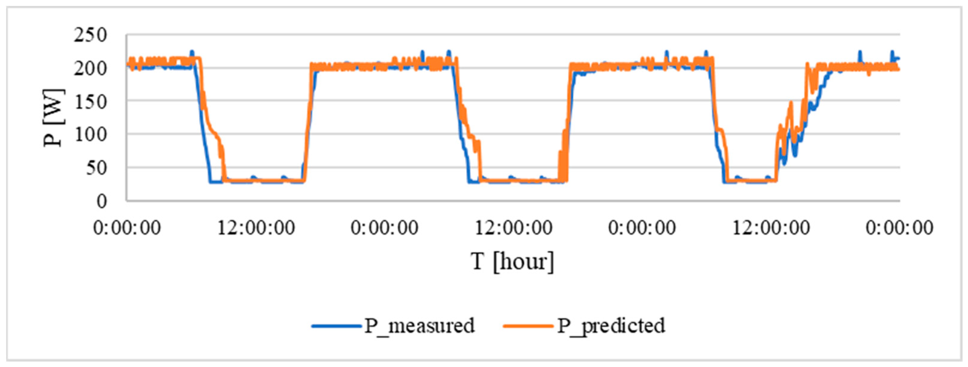
Following a similar verification procedure to the previous case, Figure 17 presents a comparison between the measured and predicted data. The blue curve represents the measured data, while the orange curve represents the predicted data.

During the last test, the measured and predicted current profiles were almost identical, with only minor deviations observed. These deviations can be attributed to both measurement and prediction model errors. The high levels of accuracy shown in Table 9 demonstrate the accuracy and reliability of the model. Similar to the previous case, slight variations were observed in the nighttime measurements, which were reliably removed by the prediction model. This confirms the robustness and potential of the artificial neural network-based model for predicting lighting consumption.

4.3.3. Comparing the Accuracy of Individual Models for Light Intensity

The prediction model was evaluated using three basic metrics: RMSE, error and the correlation between the measured and predicted values. Table 9 shows the individual parameters for each model.

Based on the results presented in Table 9, the model for the 175 lx value has the highest accuracy, corresponding to an RMSE error value of 4.04 W and an error of −1.34%. Although this value is slightly higher than that of the 140 lx value, the other metrics clearly demonstrate its dominance, allowing us to conclude that this model is the most accurate.

The other two models, however, achieve excellent results with corresponding RMSE and error values. It can be concluded that all models provide excellent predictions and can be considered valid and reliable.

From the perspective of the correlation coefficients, it is evident that there is a high level of correlation between the measured and predicted values. The correlation coefficients reach values above 0.93, which is an excellent result from a statistical point of view. This further confirms the suitability and accuracy of the models. Correlation coefficients exceeding 0.93 signify a strong positive relationship, statistically supporting the model’s ability to capture the underlying trends in the data.

The final step was to test the robustness of the models to different input values. Each model was tested on a large number of different inputs over a wide range. Based on these results, each model predicts values corresponding to switched-off lighting in the range of around 29 W for high values of external intensity in the range of 20,000–1,000,000 lx. This confirms the robustness of the models and that they are well designed and processed and can be used for all possible values of external intensity.

5. Determination and Verification of the Prediction Curve for Internal Lighting in the Interval of 100–200 lx

This section describes the use of predictive models to predict lighting consumption in the 100–200 lx range. Using a similar approach to the previous sections, a predictive model has been developed based on regression analysis and artificial neural networks.

5.1. Regression Model

Because it is possible to see that coefficients β₁ … β₃ are almost the same, experimental measuring in the range of 100–200 lx was performed. Coefficient β₀ was determined according to previously mentioned data by measuring consumption without daylight. By approximating these measured values, the linear dependence was determined, which can describe this range. Based on this curve and combined with the results of the regression analysis, it is possible to determine the consumption curves for any lighting set in the workspace.

Electricity consumption was measured at regular intervals. Then, a straight-line model (linear regression)was created to see how the current’s magnitude affects the light intensity. The higher regression coefficients, b₁–b₃, were not very different, and, for this application, the coefficients were calculated as an average. The combination of these two functions created the prediction function, which allows for the prediction of the lighting consumption in intervals of 100–200 lx.

Based on the measurement data, a linear regression curve was prepared using the following equation:

$${\beta }_0=-33.083+1.256\times E_{set}$$

(19)

The combination of function (Equation (19)) and the average values of the coefficients B1–B3 from the previous part can create the function for predicting the consumption within the interval 100–200 lx. This function is as follows:

$$P={\beta }_0+\left(-0.084\right)\times E_{out}+\left(3.4\times {10}^{-5}\right)\times E_{out}^2+\left(-2.7\times {10}^{-8}\right)\times E_{out}^3$$

(20)

This function fulfills all the requirements for quality assessment and applicability in the process of predicting lighting consumption.

Verification of the Accuracy of the Prediction Function

Tests have been carried out for a variety of scenes and data volumes. The graphs below have been selected for illustrative purposes only. The tests were carried out on 250 different combinations to ensure the unambiguousness and independence of the tests.

In order to assess the resilience of an indoor lighting consumption prediction algorithm, a series of tests were conducted within a range of lighting intensities, spanning from 100 lx to 230 lx, with increments of 10 lx. The 100 lx represents ambient lighting conditions, while 230 lx represents the intensity under full artificial lighting.

Table 10. Errors of models for interval 100–230 lx.

	RMSE [W]	Error [%]	r [−]	R2 [−]
100	11.800	2.500	0.959	0.920
110	12.540	2.910	0.957	0.916
120	12.810	2.980	0.954	0.910
130	12.020	3.000	0.951	0.904
140	11.407	5.762	0.956	0.914
150	11.546	7.891	0.954	0.911
160	12.390	9.000	0.948	0.899
170	14.344	12.509	0.950	0.902
180	17.003	14.998	0.947	0.896
190	20.310	16.000	0.942	0.887
200	24.841	20.336	0.939	0.882
210	30.020	23.185	0.935	0.874
220	36.039	26.154	0.931	0.866
230	42.898	29.243	0.926	0.857
Average	19.283	12.605	0.947	0.897

, shown below, presents a summary of the error metrics for the algorithm. The verification was carried out in a similar way as those undertaken above for the verification of prediction functions (Equations (16)–(18)). In the following figures, the curve of the electric current is measured and calculated, according to Equations (19) and (20) for three selected values (130, 160 and 190 lx). The blue curve represents the measured values and the orange curve represents the calculated values, according to Equations (19) and (20). In the following Figure 18, Figure 19 and Figure 20, the measured and calculated electric currents for the values 130, 160 and 190 lx are shown.

Although the average error is greater than that observed when the algorithm was evaluated under specific lighting conditions, the relatively low RMSE (19.283 W) and error rate (12.6%) indicate that the algorithm is sufficiently robust for determining energy consumption within the specified range. It is of note that the algorithm’s capacity to provide accurate predictions even outside its primary design range serves to demonstrate its robustness.

The analysis of error trends indicates a linear increase in error with increasing lighting intensity. This indicates that the accuracy of the predictions declines as the intensity of the light increases. Nevertheless, within the anticipated interval and its surrounding boundaries, the error remains relatively low.

The evaluation demonstrates that the algorithm exhibits adequate robustness and resilience within the specified range of lighting intensities. Furthermore, its capacity to maintain low error rates even beyond its primary design range serves to highlight its suitability for applications in indoor lighting consumption prediction.

Based on the results in Table 8, it is obvious that this approach provides the same accuracy as the prediction for the levels of 140, 155 and 175 lx.

5.2. Neural Network Model

A similar approach to that described in Section 4.3 was used to develop a model for the 100–200 lx lighting consumption range. The process began with data preparation for processing in MATLAB R2020b. After data cleaning procedures were applied, the data were imported into the MATLAB environment and then split into training, test and validation sets using a random sampling technique. The split ratio used was 70% for training, 15% for testing and 15% for validation.

The following Figure 21 shows the measured data, represented as blue points, and the orange curve represents their approximation using a neural network. As the input data were used for the intensity range 100–200 lx, there is a larger spread of values, which also leads to a larger error in the final prediction.

The results show that a waveform has been achieved that passes through the centre of the measured data. This indicates an optimum relationship between input and output. Due to the greater variance of the input data, lower accuracy values were obtained than for the individual models. Overall, the following parameters were achieved: a RMSE of 12.83 W, a correlation coefficient of 0.863 and an R² coefficient of 0.744. From these data, it can be seen that, even for a given range, a high level of prediction is still achieved.

During the verification process, it was discovered that, due to the wide range of values for the switched-on lighting (E = 0 lx), the model approximation set the level of the consumed current to 163 W for the given value. A problem arises because these values are not comparable for higher or lower values of the set intensity, which leads to the introduction of a large error.

To overcome this problem, a similar principle was used as in the regression analysis, where the coefficients of the neural network for small intensity values were adjusted to match the predicted off-mode intensity. After this adjustment, the model achieved better accuracy parameters, which are demonstrated in the accuracy verification section below, where they are described in more detail.

Verifying the Accuracy of the Prediction Function

Tests were carried out for a variety of scenes and data volumes. Figure 22, Figure 23 and Figure 24 below are selected for illustrative purposes only. The tests were carried out on 250 different combinations to ensure the unambiguousness and independence of the tests.

To verify the accuracy and applicability of a function, the verification was performed on three selected values of the internal lighting settings (130, 160 and 190 lx). The verification was carried out in a similar way to the verification of the predictive functions above. The following figures show the measured curve and the predicted curve of the electric current using ANN. A blue curve represents the measured value and an orange curve represents the predicted value.

Since the predicted value for off lighting was 163 W for each intensity, but the actual measured values were different (130 lx: 124 W, 160 lx: 145 W, 190 lx: 207 W), the ANN coefficients were corrected, so that, for small intensity values, the predicted value was at the level corresponding to the measurement. This approach was possible because the lighting was switched on and the external intensity was zero, which did not affect the prediction function. The coefficients were only adjusted for the outdoor intensity range of 0–200 lx. The following Figure 22, Figure 23 and Figure 24 show the measured and predicted current waveforms. The resulting metrics are shown in

Table 11. Errors of models for the interval 100–200 lx.

	Without Correction				With Correction
E [lx]	RMSE [W]	Error [%]	r [−]	R2 [−]	RMSE [W]	Error [%]	r [−]	R2 [−]
100	79.457	55.611	0.907	0.823	6.680	8.170	0.951	0.904
110	79.457	55.611	0.941	0.885	7.040	8.170	0.955	0.912
120	55.044	40.252	0.927	0.859	7.540	7.354	0.961	0.924
130	35.300	28.200	0.922	0.850	7.880	6.710	0.966	0.933
140	21.938	17.514	0.989	0.978	7.716	5.962	0.969	0.939
150	13.245	10.135	0.981	0.962	7.882	5.386	0.971	0.943
160	8.930	6.400	0.962	0.925	8.570	5.030	0.975	0.951
170	11.579	3.357	0.971	0.943	8.350	4.474	0.976	0.953
180	18.606	3.958	0.973	0.947	8.680	4.138	0.981	0.962
190	29.660	8.610	0.975	0.951	8.940	4.080	0.987	0.974
200	48.380	13.140	0.974	0.949	9.122	3.706	0.975	0.951
210	71.127	21.721	0.969	0.939	9.220	3.610	0.969	0.939
220	99.114	32.962	0.965	0.931	9.380	3.594	0.961	0.924
230	132.341	46.863	0.951	0.904	9.470	3.658	0.960	0.922
Average	50.298	24.595	0.958	0.918	8.319	6.401	0.968	0.938

.

In order to assess the robustness of an algorithm for an indoor lighting control application, a test was conducted utilizing a range of lighting intensities, spanning from 100 lx to 230 lx.

100 lx: This represents the amount of ambient light present in the environment.

230 lx: This represents the light intensity when full artificial lighting is turned on.

Table 11 below presents a summary of the error metrics for both the uncorrected and corrected algorithms.

After extensive test iterations, it was possible to evaluate the results and compare the effectiveness of the two models.

The results indicated a notable enhancement in performance when the correction algorithm was applied. The corrected algorithm achieved a substantially lower RMSE of 8.316 W and an error rate of 6.4% in comparison to the uncorrected algorithm, which exhibited an RMSE of 50.298 W and an error rate of 24.0%. Furthermore, the corrected algorithm exhibited higher r and R² values, indicating a stronger relationship between predicted and actual energy consumption.

These results indicated that the corrected algorithm was well-designed and capable of accurately predicting energy consumption across the entire range of input values. Notably, even at the maximum illumination level of 230 lx, the corrected algorithm maintained a low error rate of 9.4% and a RMSE of 9.47 W. This highlights the algorithm’s robustness and ability to deliver accurate predictions beyond its training range.

In contrast, the uncorrected algorithm’s performance was significantly affected by errors and the aforementioned factors. The high RMSE of 50.298 W and the error rate of 24.0% indicated a significant discrepancy between the predicted and actual energy consumption. This lack of robustness precludes the algorithm’s applicability in real-world scenarios.

The analysis shows that the ANN-based models with correction achieved significantly better accuracy than the models without correction. The average improvement in accuracy of the ANN models were 78% by 130 lx, 5% by 160 lx and 70% by 190 lx, compared to the regression model. This observation can be explained in the following way:

• Accurate approximation by the neural network: In this particular case, the neural network (NN) was able to accurately approximate the real value of energy consumption. This means that the predicted value without correction was already so accurate that the effect of the correction was minimal.
• Confirmation of the correctness of the approach: This phenomenon perfectly demonstrates and confirms the correctness of the chosen approach and solution. The prediction function predicts the value with the required accuracy without the need for correction.
• Proof of the correction function: At the same time, the concept of correcting the initial values is confirmed. Although, in this case, the correction was minimal, its implementation ensures that the results are provably correct, even in cases where the predicted value is less accurate.

6. Discussion

Two different approaches with different characteristics and levels of complexity were implemented to address the problem. This section focuses on the comparison between the regression model and the ANN-based model. The comparison between the models is summarized in

Table 12. Comparison of the regression and ANN models.

	ANN Model			Regression Model			Difference [%]
	RMSE [W]	r [−]	R2 [−]	RMSE [W]	r [−]	R2 [−]	RMSE	r [−]	R2 [−]
140 lx	4.25	0.984	0.968	9.63	0.965	0.931	55.85%	1.96%	3.96%
155 lx	4.70	0.982	0.964	9.82	0.966	0.933	52.12%	1.66%	3.34%
175 lx	3.80	0.987	0.974	9.48	0.973	0.947	59.97%	1.42%	2.86%
100–230 lx	8.319	0.968	0.938	19.28	0.946	0.896	56.85%	2.33%	4.69%

below.

After extensive test iterations, it was possible to evaluate the results and compare the effectiveness of the two models. The analysis shows that the ANN-based models achieved significantly better accuracy than the regression models. The average improvement in accuracy of the ANN models was about 50%, compared to the regression model. The improved accuracy of the ANN model was due to its superior ability to approximate input data. Unlike the regression model, which performed linear approximation, the ANN could capture complex non-linear relationships between input and output variables. This led to an automatic improvement in accuracy.

Regression Model:

• Limitations

The regression model produced satisfactory results within a limited range of input values. However, it diverged at higher values (above 10,000 lx) and calculated negative energy consumption values, rendering the results impractical and unusable for practical solutions.

• Causes of incorrect operation

The incorrect functioning of the regression model at higher input values was due to the nature of the polynomial approximation it used. Polynomial functions tend to diverge when extrapolating outside the range of the training data.

• Practical application

The use of the regression model must therefore be limited to the area where the results are meaningful and relevant to the problem being solved. However, even in this limited domain, its use is problematic and requires additional verification and validation of the results.

ANN model

The ANN model successfully overcame all the shortcomings of other models. It could provide correct results, even for large values of outdoor illuminance. These results correspond exactly to the switched-off lighting, which is absolutely correct from the point of view of the consumption and operation of the lighting system.

The main benefits of the ANN model are as follows:

• Accuracy: it can accurately predict energy consumption even at high outdoor light levels.
• Speed: the calculation is done by multiplying constants, which is extremely fast with today’s computing power.
• Stability: it is robust to errors and unstable behavior in extreme conditions.
• Adaptability: the ANN model is adaptive and can adapt to different types of lighting systems.
• Robustness: the model is robust and resistant to errors in the measured data.
• The disadvantages of the ANN model are as follows:
• Training: training the model can take quite a long time, depending on the size and complexity of the training data set.
• Difficulty: implementing and understanding the ANN model can be more challenging for some users.

The ANN model represents a significant advance in the prediction of lighting energy consumption. Its advantages, such as accuracy, speed and stability, make it an ideal tool for optimizing the energy consumption and operation of lighting systems.

From a practical point of view, the ANN-based model is a much better choice for predicting lighting energy consumption. Its higher approximation capability and robustness to divergence ensure accurate and reliable results, even at high levels of external lighting intensity.

Laboratories

The proposed lighting consumption prediction algorithm has been designed with the intention of predicting and optimizing energy consumption in office spaces. However, it is possible that it could be adapted for use in laboratories with certain considerations. Due to the nature of the work and the safety requirements in laboratories, lighting is not typically controlled based on external lighting conditions. Additionally, it is worth noting that standardized lighting levels in laboratories are often higher than in office spaces, reaching up to 1500 lx [49].

Because the prediction algorithm will have to operate within a narrow range, it is likely that the values calculated using the predictive model would be practically identical to those in an uncontrolled system.

Adaptations for Laboratories:

In the case of laboratories, the algorithm’s primary function of predicting lighting consumption based on external light levels is not applicable. Instead, the focus should be on maintaining standardized lighting levels while ensuring the safety and comfort of laboratory personnel. This can be achieved by implementing the following adaptations:

• Fixed lighting levels: setting lighting levels to the standardized values required for laboratory operations.
• Occupancy detection: utilizing occupancy sensors to detect the presence or absence of laboratory personnel.
• User overrides: providing manual controls for laboratory personnel to override the automated system if necessary for specific tasks or experiments.

7. Conclusions

This article presents a comparative analysis of two prominent machine learning techniques for predicting electricity consumption in buildings: polynomial regression and ANN. The focus is on assessing their practical applicability and accuracy in predicting lighting consumption in an administrative building.

Following a comprehensive review of the existing literature on predicting electricity consumption in buildings and systems, the article delves into the theoretical foundations of both approaches. This includes an explanation of the underlying principles of polynomial regression and ANNs, as well as the procedures for determining the correlation coefficient, coefficient of determination and error. Using this theoretical framework, the paper describes the development of two different models for predicting lighting consumption.

Both models use measured outdoor lighting intensity data as the primary input variable. For the polynomial regression model, this data is subjected to regression analysis, resulting in a function that captures the relationship between outdoor lighting and building lighting consumption. Similarly, the ANN model is trained on this data, allowing it to learn the complex relationships between external lighting and internal consumption.

The analysis considers three specific lighting levels. Two levels correspond to the established EN 12464-1 standard, ensuring compliance with lighting regulations. The third level is based on the subjective wellbeing of the building’s occupants, with the aim of achieving a balance between energy efficiency and occupant comfort.

The validation process for both models included the following steps: the measurement of external light intensity, wherein actual outdoor light levels were measured; electric current prediction, wherein the prediction function of each model was used to calculate the expected current based on the measured external light levels; and comparison with measured current, wherein the calculated current values from both models were compared with the actual measured values of the electrical current for lighting consumption. The accuracy of each model was assessed using several statistical metrics, namely the RMSE, the error, the correlation coefficient and the coefficient of determination.

The ANN model consistently outperforms the polynomial regression model on all evaluation metrics. The ANN model achieves a significantly lower RMSE (4.76 W vs. 14.49 W), a lower error percentage (0.56% vs. 8%) and higher values for both r (0.954 vs. 0.93) and R² (0.910 vs. 0.866).

This superior performance suggests that the ANN model is better equipped to handle the inherent non-linearity in the relationship between outdoor lighting intensity and building lighting consumption.

The evaluation process was repeated, to assess the performance of the models in predicting lighting consumption within a specific range (100–230 lx). The results follow the same trend as the overall evaluation: a lower RMSE (8.316 W vs. 19.28 W), a lower error percentage (6.4% vs. 12.6%) and higher values for both r (0.968 vs. 0.946) and R² (0.938 vs. 0.896). The ANN model again shows superior performance in this specific lighting domain, further confirming its suitability for this task.

The validation process demonstrably confirms the superiority of the ANN model for predicting lighting consumption in this study. The ANN model consistently achieved higher accuracy than the polynomial regression model across all evaluation metrics. This improved accuracy can be attributed to the ANN’s ability to capture complex, non-linear relationships within the data, which is consistent with the theoretical strengths of ANNs for modelling such scenarios.

The results of this study suggest that there are significant benefits to incorporating ANNs into lighting system management. The developed ANN model shows a high degree of accuracy in predicting lighting consumption. This accurate predictive capability is critical for optimizing overall building operations. Using this data allows for the following benefits:

• Improved operational planning: by accurately predicting lighting consumption, building managers can more effectively prepare operational strategies.
• Improved integration of renewable resources: the ability to predict lighting demand enables the better integration of renewable energy sources.
• Improved building energy efficiency: the accurate prediction of lighting consumption enables building managers to implement strategies that optimize energy use, resulting in a more energy-efficient building.
• Reduced greenhouse gas emissions: as a direct result of increased energy efficiency, greenhouse gas emissions associated with building operations are also reduced.

As with any predictive model, the accuracy of the ANN model is inherently linked to the quality and quantity of the input data. This study highlights the importance of focusing on acquiring a larger and more comprehensive dataset for future work. By increasing the number and variety of training data points, it is possible to achieve even better predictive parameters. This will ultimately lead to more refined and reliable results that can be effectively implemented in practical applications.

Directions for future works include the following:

• Extending the data collection period to capture seasonal variations in lighting demand.
• Including additional relevant data points, such as weather conditions or occupancy patterns.
• Exploring data augmentation techniques to artificially increase the size and diversity of the training data.
• Combination of lighting system with other systems, e.g., control of the shutters and detection of persons.

By incorporating these improvements, future research can further refine the ANN model and cement its role as a valuable tool for optimizing building energy efficiency and reducing environmental impact.