Abstract
This work evaluates the ventilation resilience of the combined personalized ventilation (PV)-mixing ventilation (MV) system when implemented in a typical office space. This resilience is first evaluated by monitoring the ability of the PV devices when designed at different supply flow rates to maintain acceptable levels of CO2 at the occupant’s breathing zone when the MV system is subjected to a shock. The shock considers a malfunction of the MV system for periods of 3 h and 6 h, and at shutoff percentages of MV fan flow of 100% and 50%. This is followed by evaluating the resilience of the MV system when the PV air handling unit is shutoff for short periods. The following three aspects of resilience were calculated: the absorptivity, the recovery, and the resilience effectiveness. To monitor the CO2 temporal variation at the breathing zone, a computational fluid dynamic model was developed and validated experimentally. It was found that the resilience effectiveness varied between 0.61 (100% MV shutoff for 6 h and PV at 4 L/s) and 1 (50% MV shutoff for 3 h and PV at 13 L/s). Additionally, CO2 build-up and recovery took minutes during MV malfunctions and seconds during PV malfunctions.
1. Introduction
As people are spending the majority of their time indoors, it is imperative to ensure that indoor spaces are adequately ventilated to safeguard the health and well-being of people [1]. The quality of the indoor air depends not only on the design of the air conditioning (AC) system, but also on its proper and permanent operation. It is of great importance to consider extreme, unexpected events, which have the potential to impact the functioning of the AC system and negatively affect the indoor air quality (IAQ) [2]. Hence, the quality of the indoor air should be studied while considering the following two aspects: (1) the proper design of the ventilation system and (2) its resilience when subjected to unpredicted events [3].
For a proper design, the air conditioning (AC) system should supply the proper amount of outdoor air to simultaneously dilute the contaminants present in the indoor space and provide breathable air to the occupants. In addition, the outdoor air should be conditioned prior to supplying it into the space for comfortable indoor conditions, which renders the use of such systems energy intensive. In office spaces, many efforts have been made to design novel ventilation systems with the aim of ameliorating the breathable air quality and thermal comfort of workers with low energy consumption [4,5,6].
Personalized ventilation (PV) is one of the most recommended ventilation strategy when considering energy efficiency as follows: it supplies clean, cool air directly toward the occupant breathing zone through an air terminal, thus enhancing the inhaled air quality and thermal comfort [7,8]. In addition, such technology gives the occupants the opportunity to control their own microclimate according to their personal needs and preferences [9,10]. PV systems are found in many studies to be energy effective compared to conventional AC systems since they allow relaxing the background temperature and contaminants’ concentration to threshold limits [11,12]. This decreased energy demand leads to lower greenhouse gas emissions associated with the energy production of total air volume ventilation systems. Consequently, the implementation of PV devices contributes to eco-friendly building practices by promoting energy efficiency while providing the necessary air quality and thermal comfort for the occupants. Many studies investigated the effectiveness of using PV devices to enhance the thermal comfort and the air quality of occupants at a reduced energy cost. For example, Cermak et al. [13] conducted an experiment in a room ventilated by a mixing ventilation (MV) system and was comprised of two occupants equipped with PV terminals. They evaluated the effectiveness of the PV devices in providing acceptable inhaled air quality compared to the case when MV was used with no PV. They found that the use of PV in conjunction with MV greatly decreased the concentration of pollutants and the temperature of the inhaled air with respect to the case when no PV was used. In addition, the PV device is effective for mitigating cross-contamination risks as follows: it creates a confined microenvironment around the occupants and protects them from the contaminants present in the macroclimate [14]. Pantelic et al. [15] conducted experiments on a healthy occupant utilizing a PV device in a space conditioned with a MV system. They studied the effect of using the PV on the direct exposure to cough droplets released from a source inside the space. They found that the PV was able to reduce the exposure to cough-released droplets by a minimum of 41% compared to the case when no PV was used.
The design (size and position) as well as the operating conditions (supply flow rate and temperature) of the PV device are designed based on the expected operation of the background AC system and concentration of indoor contaminants. Shinoda et al. [16] proposed a multi-functional personalized PV device equipped with a filter, a UVGI component, and a Peltier cooling element. They performed human-centered experiments to evaluate the human-perceived air quality under normal operation of the proposed device. Similarly, Saheb et al. [17] conducted numerical comparison tests for the PV devices when combined with two different background ventilation systems (MV and displacement ventilation (DV)) under normal operation without disturbances. They found that the PV combined with MV was more effective in improving the air quality of users compared to PV combined with DV. Xu et al. [18] evaluated different PV arrangements and their effect on the inhaled air quality of the user when the background MV system was operating at normal conditions. They found that the efficiency of clean air delivery from the PV device varied slightly depending on its position. However, throughout the lifetime of the office building, there are instances when the background AC system is subjected to a malfunction or sudden shutdown that cannot be anticipated, hence, it cannot be prevented. These events are due to power blackout [19], irregular maintenance [20], or extreme weather events [21]. This causes the accumulation and build-up of the background CO2 level, which threatens the occupants’ health once they get entrained with the PV jet deteriorating, and thus the inhaled air quality. Hence, it is of great interest to evaluate the extent to which the PV devices are able to guarantee a good level of IAQ for the occupants under such shocks. This characteristic in any ventilation system is termed “ventilation resilience”, and is defined by Al-Assad et al. [22] as the ability of the ventilation system to withstand and absorb the shock and maintain IAQ design conditions. The latter studied the ventilation resilience of the demand-controlled ventilation systems in educational buildings in Belgium. They found that the demand-controlled ventilation system has a similar resilience to a constant air volume regarding CO2, but from 53% to 62% worse for VOCs. The parameters that affect the degree of the shock and its impact on the PV’s ability to maintain an acceptable breathable air quality are (1) the severity and (2) the duration of the shock. For instance, the components of the background ventilation system can be in a complete failure mode (leading to the total interruption of the supply of clean outdoor air) or a partial failure mode (leading to a decrease in the rate of supply of clean outdoor air). These failures may be caused by clogged filters in the system ducting due to an irregular cleaning or replacement, a malfunction in the AC fans due to blades or motor issues, or an unexpected power outage [23]; moreover, the failure state can persist for different periods of the entire occupied time [24]. Hence, the shock percentage and the time elapsed between the beginning and the end of the shock should be taken into consideration when assessing the ventilation resilience of the PV device. Al-Assad et al. [25] investigated a variable air volume ventilation system in an open-plan office, and assessed its ventilation resilience against power outages for different shock durations. They reported that this ventilation system was resilient for up to 15 min after a power outage of the ventilation system.
The existing literature studies have investigated the effectiveness of PV devices in maintaining acceptable air quality levels at the occupant breathing zone assuming normal MV operation and under a pre-defined background CO2 concentration. They did not study the air quality levels at the user breathing zone during a malfunction of the MV system for different PV design conditions. Furthermore, they did not account for the impact of a sudden malfunction of the air handling unit responsible for supplying fresh air to the PV device. The aim of this work is to evaluate the ability of PV devices to maintain acceptable CO2 levels at the breathing zone of the occupant when operated at their design supply flow rate with an MV system in an office space undergoing different shock degrees. The shock considers the following: (i) a malfunction of the MV system and accounts for different malfunctioning durations and severity (different shutoff percentages) leading to a CO2 accumulation in the macroclimate, and (ii) the malfunction of the PV devices while the MV system is operational at its design conditions. To the authors’ knowledge, no other studies have explored the combined resilience of MV and PV systems across various levels of shock, particularly in the context of sudden malfunctions affecting the air handling units responsible for supplying both the MV and the PV systems. The resilience behavior of the combined PV–MV system is studied according to the following three aspects: absorptivity, recovery, and impact. To achieve these objectives, a 3D computational fluid dynamic (CFD) model of the domain is modeled using ANSYS fluent. The predictions of the CFD model are validated experimentally and used to evaluate for different PV design flow rates and shock degrees, the ventilation resilience of the combined PV–MV system. This study presents insights into the ability of the PV devices at different design flow rates to react to and recover from unexpected mechanical disturbances that might influence their main role in providing clean air to the occupants. To answer those specific objectives, this paper starts with a detailed description of the domain representing the office space, with the four occupants equipped with PV devices and PC monitors each. The dimensions of each component of the domain, as well as its operating conditions, are presented, justified, and benchmarked with the previous works.
2. System Description
The space under study is a typical office space of dimensions 3.2 m 3.5 m 2.6 m conditioned with a conventional MV system served by its own air handling unit. The latter supplies an ACH equal to eight inside the office as adopted in the other literature studies incorporating PV devices in a MV-ventilated office space [26,27]. The MV air distribution system consists of a ceiling-mounted square supply diffuser (600 mm 600 mm) and an outlet grille (600 mm 600 mm). The MV system supplies a mixture of fresh outdoor air and recirculated air with a CO2 concentration of 540 ppm capable of maintaining a relaxed background CO2 level of 1100 ppm inside the space [28]. The office is considered densely occupied, with four occupants sitting around a table at close proximity with a separation distance of 0.8 m between them, as shown in Figure 1. This distance is adopted in the previous literature studies when considering a critical condition of close seating distance between occupants [29,30]. The distribution of the occupants inside the space is common in published research works [31,32], and is compliant with the office space planning guidelines [33]. Hence, four occupants are sitting in the middle of the office space around a table having the following dimensions of 2.0 m 1.8 m with 0.7 m elevation from the floor level [29]. Each occupant is doing a sedentary activity on a PC monitor having a length of 0.45 m, a height of 0.34 m and a width of 0.03 m, as adopted in the other literature studies that modeled an office configuration [34,35]. Horizontal table-mounted PV devices having a nozzle diameter of 10 cm [27,35] are assisting the MV system and are placed at a distance of 40 cm in front of each occupant face [9,36,37], as shown in Figure 1. The PV nozzles are served by their own air handling unit as follows: they supply clean, cool air obtained from an adjacent clean source. Hence, the MV and PV devices operate independently since each is connected to its own air handling unit with a distinct ducting system, filters, and power supply electric sources. The breathing activity of the PV users was neglected in this work due to its insignificant effect on the PV-supplied jet, hence on the CO2 accumulation in the breathing zone. This was reported by Russo et al. [38], which used an experimentally validated CFD model to study the effect of breathing on the inhalation exposure of a PV user. They demonstrated that for a steady PV supply flow rate higher than 2.4 L/s, the PV core jet, hence, the inhalation exposure was not affected by the breathing disturbances.
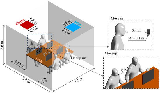
Figure 1.
Illustration of the studied office space showing the occupants, the office furniture, and a closeup to the occupant breathing zone and the distance between two consecutive occupants.
2.1. Investigated Case Studies
Shocks are defined as unexpected events that occur without prior planning or knowledge of the occupants or designers and their consequences cannot be attenuated or avoided. In this work, the mechanical shock is studied, which is an event that causes a complete or partial shutoff of the mechanical ventilation system, thus preventing the sufficient supply of clean outdoor air into the space for a defined period of time. This causes a build-up of CO2 in the space, which may reach unhealthy levels and reach the occupants’ breathing zone by entrainment into the PV jet. This shock is studied in this work, and its intensity is varied to consider low, moderate, and severe degrees of shock by accounting for various (1) shock durations and (2) shutoff percentages, as summarized in Table 1A. It is noteworthy to mention that the shock degrees are quantified according to the definition of Al-Asaad et al. [22], and they vary from 0.16 being low (50% MV shutoff for 3 h), 0.33 being moderate (100% MV shutoff for 3 h and 50% shutoff for 6 h), and to 0.67 being severe (100% MV shutoff for 6 h).

Table 1.
The different studied combinations of PV–MV resilience for (A) MV malfunction and (B) PV malfunction.
- (1)
- Shock duration: The duration of the MV malfunction was studied for a duration of 3 h and a duration of 6 h, representing 30% and 66% of the total working hours in the office space (from 08:00 to 17:00), respectively;
- (2)
- Shutoff percentages: The failure degree of the MV system was studied by accounting once for a complete shutoff (100% shutoff), meaning no air was supplied by the MV system, and once for a half-shutoff (50% shutoff), meaning the MV system was operating at half its normal capacity (supplying half the normal air flow rate).
Additionally, the PV devices are typically designed in combination with an MV system for different supply flow rates, which affect their core jet and its interaction with the surrounding environment. High design flow rates may increase the entrainment of background CO2 species, while low design flow rates may worsen the dilution of species [39]. Therefore, the ventilation resilience of the PV–MV system is examined at different flow rates design conditions of 13 L/s, 9 L/s, and 4 L/s. It is worth mentioning that this range of PV flow rates was found to maintain acceptable thermal comfort and local sensations to the users for a background temperature of 26 °C and a PV supply temperature of 23 °C [40]. Note that this temperature combination is widely adopted in the literature when evaluating the effectiveness of PV devices in uniformly conditioned spaces [41,42,43]. Furthermore, the 3 °C temperature difference between the average indoor temperature and the PV supply temperature is highly recommended to prevent thermal discomfort and draft sensation for the users [27,42,44].
Furthermore, the PV shutoff is studied while the MV system is operational. In this case, the PV devices are completely turned off for a duration of 2 min (due to the fast build-up and recovery periods in this case), while the MV system is operating normally (supplying at 8 ACH) during the entire occupied period (See Table 1B).
2.2. Criteria for Ventilation Resilience Assessment
To assess the ventilation resilience of the combined PV–MV system, two steps are adopted as per Al-Assaad et al. [45]. In the first step, the MV system is shut down for a period of time and a percentage corresponding to the studied case (see Table 1). In the second step, the temporal variation in the CO2 at the breathing zone of one occupant is observed and monitored. It is worth mentioning that, although the arrangement of the MV diffusers in the studied domain is not symmetrical (see Figure 1), it is typically adopted [27,46]. It ensures symmetrical conditions inside the space due to their low air supply momentum, hence the CO2 build-up is the same at the breathing zone of all the occupants; therefore, the temporal CO2 variation can be monitored for only one occupant and is deemed applied to all of them. Finally, the following three aspects of PV ventilation resilience are evaluated:
- 1.
- The absorptivity effectiveness (): This index evaluates the potential of the PV system to absorb the shock. It is quantified as the duration, during which the CO2 at the breathing zone of the occupant builds up from its recommended threshold value of 1000 ppm [47] until reaching a peak concentration value. This index is calculated as follows [45]:where is the absorptivity time and (hours) is the occupied period (9 h). It is noteworthy to mention that values of close to 0 indicates that the exposure to CO2 is severe since its concentration in the breathing zone of the occupant reaches peak value in a short period of time exposing the occupant to CO2-laden air above the threshold values for a long period of time. However, values of closer to unity indicate a better resilience of the PV device since the latter is dampening the high CO2 concentration at the breathing zone of the occupant for a longer period of time;
- 2.
- The recovery effectiveness (): This index evaluates the duration it takes for the PV device to recover from the shock. It is quantified as the duration expanding between the instant at which the shock ends and the instant at which the average CO2 concentration at the breathing zone of the occupant reached threshold values (1000 ppm). This index is evaluated as follows [45]:where is the recovery time and (hours) is the occupied period (9 h). When the value of is close to 0, the recovery time is long, which indicates a longer exposure to CO2-laden air, above the recommended threshold" value, at the breathing zone of the occupant. However, for values close to unity, the recovery time is short indicating that the concentration of CO2 at the breathing zone reaches healthy levels quickly after the shock on the MV system ends;
- 3.
- The resilience effectiveness (): this index evaluates the impact of the shock, which is the duration during which the occupant was exposed to unhealthy CO2 levels compared to both the case of no shock (best case scenario) and the case of no PV (worst-case scenario). This index is calculated as follows [45]:where the is an integration of the CO2 curve above 1000 ppm with the correlative time duration [48]. Hence, the is an evaluation of the when the system is under one of the studied shocks presented in Table 1, the is an evaluation of the for the case when the same shock was applied but without the use of PV, and the is the when no shock occurs and both the MV and PV are at normal operation.
Note that for each of these terms, the is evaluated at the breathing zone of the occupant. If the value of approaches 1, then the conditions at the breathing zone of the occupant are close to those obtained when no shock occurs, hence the PV–MV system demonstrates the highest level of resilience. In this case, the shock has the least impact on the effectiveness of the combined PV–MV system. However, if the value of approaches 0, then the conditions at the breathing zone of the occupant are close to those obtained when no PV is used hence, the PV–MV system exhibits the lowest resilience. In this case, the shock has a substantial impact on the effectiveness of the combined PV–MV system.
3. Numerical Methodology
The described system was characterized by complex flow interactions between the PV jet, the mixing flow profile created by the MV system, the different heat fluxes, and their corresponding thermal plumes generated inside the space (occupants, PCs, walls, and ceiling). Consequently, such interactions cannot be simulated by developing simplified mathematical models, and a 3D CFD simulation tool should be used to solve complex and transient flow interactions. This tool had been widely used in the literature to simulate the complex flow interactions and predict the air quality in indoor spaces, such as offices [49,50,51], meeting rooms [52,53,54], and classrooms [55,56,57], and showed accurate and reliable results. In this work, a CFD model was developed using the commercial software ANSYS (version 19.2) [58] to solve for the velocity, temperature, and species transport in the space. Then, a parametric study was conducted to evaluate the ventilation resilience of the PV when used with a MV background system for different PV base design flow rates associated with the MV system and shock degrees.
3.1. CFD Model
The computational fluid domain developed in ANSYS was represented in Figure 1 where the diffusers of the MV system, the occupants around the table, their PC monitors and the PV devices were replicated. For an accurate prediction of the flow properties, the domain was carefully meshed, as shown in Figure 2. The discrete grid elements were set to have a tetrahedral unstructured geometry and their size were varied according to the boundary face complexity. A grid size of 1.5 cm was assigned for the occupants and for the PV inlet faces. In addition, the MV supply and outlet surfaces were meshed with a grid size of 2 cm, while the CO2 sources, which are placed at the middle of each wall, were meshed with a grid size of 0.5 cm. Five inflation layers were created around the boundary surface of the manikin to accurately capture the thermal plume while ensuring that the dimensionless wall number y+ was approximately equal to 1 [59]. To accurately capture the temporal CO2 variations in the breathing zone of the occupant, a sphere of influence was created in the zone between the PV inlet face and the occupant face, as shown in Figure 2. This sphere of influence had a radius of 2 cm and a mesh size of 1.5 cm. Furthermore, to ensure that the solution of the partial differential equations at any point of the considered domain was independent of the gridding scheme, a mesh independence test was performed (Table 2). In this test, the average air velocity was calculated in the mid-plane passing through the PV device and the occupant face. This velocity was calculated for a PV supply flow rate of 13 L/s, and is considered reliable for all the operating conditions of the PV since none of them included a change in the geometry of the domain [60]. This test revealed that the adopted mesh scheme created an error of 4.5% compared to the previously tested mesh configuration and resulted in 4,230,449 number of elements and a minimum orthogonal quality of 0.41.
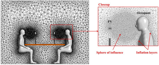
Figure 2.
The gridding scheme of the CFD model of the office space.
Table 2.
Results of the mesh independency test.
3.2. Airflow Model
The CFD solver in ANSYS fluent numerically solves the evolution of the fields of properties in space and time coordinates by solving the Navier–Stokes (Equations (4) and (5)) and energy (Equation (6)) equations, which are given by the following [61]:
Equation (4) represents the mass conservation equation. Equation (5) is the momentum conservation equation, in which the term at the left-hand side corresponds to the inertia term. On the right-hand side, the first term represents the pressure gradient, the second and third terms are the shear stress terms, and the last term represents the body forces. Where () is the density, (m/s) is the velocity vector, t () is time, () is the pressure, and () is the dynamic viscosity. Equation (6) is the energy conservation equation, in which the convective heat transfer term on the left-hand side is related to the energy transfer due to conduction (), species diffusion (), and viscous dissipation () on the right-hand side. Where () is the constant volume specific heat, () is the temperature, () is the sensible enthalpy of species i, () is the diffusion flux of species i, () is the thermal conductivity, and () is the viscous dissipation.
The solver was set to transient since the aim was to evaluate the temporal change in CO2 concentrations. The adopted time step was 0.2 s, and the simulation was set to 162,000 time steps corresponding to the total studied period of 9 h. Note that the implicit scheme was used, which had unconditional stability and put no restriction on the size of the time step, hence on the CFL condition [61]. The developed domain contains high turbulence effects generated from the interaction between the PV flow and the thermal plume from the occupants. Hence, it was imperative to select the adequate turbulence model to solve for the turbulent kinetic energy and its rate of dissipation . The RNG turbulence model was adopted since it showed the best balance between accuracy and computing time performance when predicting complex airflow interactions in indoor spaces [62]. The model was considered as a continuous fluid and was simulated by the Eulerian approach [63]. In addition, the enhanced wall treatment option was activated with the full buoyancy effect. These options were found to increase the robustness and reduce computational cost of the simulation [64]. In addition, as the temperature variation and subsequently the gradient variation in the office space were negligible, the “Boussinesq” approximation was used to account for the buoyancy effects [65]. The second order upwind scheme was used to solve the mass, energy, momentum, , , and transport equation, and the PRESTo! scheme was used to solve for the pressure equation [66]. Since the variables in the domain are time-dependent, the PISO scheme was used for the velocity-pressure coupling [67]; furthermore, the CO2 transport in the space was simulated using the species transport equation. Note that the studied domain replicated a typical office space with no large window openings hence, the radiation model was neglected. Furthermore, the numerical model was considered converged when the scaled residuals reached 10−7 for the energy and 10−5 for the remaining parameters [68].
3.3. Boundary Conditions
It is crucial to carefully select the boundary conditions on the boundary surfaces of the domain to obtain accurate results of flow field and species concentration profiles. The MV supply diffuser was set to the velocity inlet boundary condition with a supply velocity of 0.2 m/s and a specified inlet temperature of 17 °C with a calculated Reynolds number of 8000. The turbulence intensity and the hydraulic diameter were set to 6% and 0.6 m, respectively. The air supplied from the MV system contains a CO2 concentration of 540 ppm leading to relaxed macroclimate conditions with CO2 concentrations of 1100 ppm. This CO2 concentration was added as a boundary condition at the MV opening area with a mass fraction value of . As for the corresponding outlet diffuser, it was set to pressure-outlet boundary condition with zero gauge pressure. Each PV supply opening was assigned as a velocity inlet with a specified temperature of 23 °C and a velocity that varies according to the studied case, as per Table 1. The calculated average Reynold number ranged from 3500 (at 4 L/s) to 1100 (at 13 L/s). The turbulence intensity and the hydraulic diameter of the PV surface were set to 5% and 0.1 m, respectively. Note that the air supplied from the PV originated from an independent air handling unit and supplied clean outdoor air with a CO2 generation of 450 ppm. This CO2 concentration was specified as a boundary condition on the PV area with a mass fraction of . The occupants were considered as heat sources, generating 39 W/m2 while performing sedentary activities [56], which corresponds to a total heat generation of 75 W from the body of each occupant [69,70,71]. The lighting fixtures were assumed to be uniformly distributed at the ceiling level hence, to account for their generated heat, the boundary condition at the ceiling surface was set to a continuous heat flux of 10 W/m2 [72,73], and the walls were set to a constant heat flux of 15 W/m2 [27]. To ensure a uniform distribution of passive contaminants represented by the CO2 tracer gas inside the room, a CO2 source was placed at the middle of each wall. Each source was generating CO2 at an amount of 0.5 L/min, corresponding to a total generation of 2 L/min, which was equivalent to the amount of CO2 exhaled by four occupants. This approach was adopted in the previous literature studies that investigated the air quality in indoor spaces [59,74]. Note that during the shock period, the MV outlet diffuser was set to pressure-outlet to balance the supply flow rate of the PV devices and the CO2 sources.
4. Experimental Methodology
The developed CFD model used for the evaluation of the PV–MV ventilation resilience was validated experimentally. The CFD predictions of CO2 spread in the background and in the breathing zone at various degrees of shock and PV design flow rates were compared to those obtained experimentally in a controlled climatic chamber.
4.1. Experimental Setup
The experiment was conducted in a climatic chamber at AUB having the following dimensions: 3.4 m 3.4 m 2.6 m and ventilated by a MV system with diffusers having the dimensions of 0.4 m 0.4 m. The chamber was highly insulated with a wall U-value of 1.5 . The air was delivered from the MV supply diffuser at a velocity of 0.4 0.02 m/s, a temperature of 24.5 0.2 °C with a measured CO2 concentration of 520 73 ppm. A human-like thermal manikin representing a real human being was placed in the middle of the chamber. The thermal manikin was manufactured by Measurement Technology Northwest [75]. It had 20 surface segments and was able to operate in a wide range of temperatures (from −20 °C to +50 °C) and had a 700 maximum power output. The thermal manikin was controlled using “ThermDAC” control software (version 4 1 25), which was set to assign a heat flux of 39 W/m2 to each body segment of the manikin to represent a human being performing a sedentary activity with a metabolic rate of 1.2 met. A PC mock-up was placed in front of the manikin to represent the PC and was equipped with a 100 W power lamp in the inside for heat generation. Furthermore, the heat flux generated by the lighting fixtures at the ceiling level of the chamber was equivalent to 10 . Consequently, the total internal load inside of the climatic chamber was 290 W. A PV device was supplying air to the manikin breathing zone at a temperature of 23 0.2 °C, which is 3 °C lower than the average room temperature (26 °C 0.2 °C). This temperature difference was recommended and adopted in the previous literature studies to reduce draft discomfort [27,42,44]. The PV had a nozzle diameter of 10 cm and was installed at a distance of 40 cm in front of the manikin face at 1.2. m from the floor representing the breathing level. The PV was supplying at a velocity of 0.5 0.03 m/s and 1.7 0.08 m/s corresponding to a design supply flow rate of 4 L/s and 13 L/s, respectively, which constitute the highest and lowest limits of the studied PV design airflow range. The PV nozzle was equipped with a DC-fan (12 V, 48 W) and was connected to its own air handling unit, which supplied conditioned air to the breathing occupant from the sandwiched layer adjacent to the climatic chamber at a CO2 concentration of 520 73 ppm. To reduce the turbulence intensity of the PV jet supplied toward the face of the occupant, a honeycomb flow straightener and a screen were mounted downstream, and a screen was mounted upstream the flow direction. The honeycomb has a thickness-to-diameter ratio of 7.5, corresponding to a thickness of 3 cm and hole diameters of 4 mm. As for the screen layers, they had a porosity of 80% each. These dimensions were recommended to obtain optimal results [76], and were adopted in the other literature studies that built a prototype of the PV device for experimental purposes [74]. It is worth mentioning that the setup of the experiment differed from the model considered for the parametric study hence, a CFD model was developed replicating the experimental chamber with the manikin and PV positions as well as the heat loads. This approach was adopted in the previous literature studies to experimentally validate their CFD models [77,78].
Since the aim of the study was to evaluate the ventilation resilience of the combined PV–MV system, 4 constant sources of CO2 were utilized, one on the middle of each wall, to create uniform conditions inside the room as shown in Figure 3A. The CO2 sources were supplying a constant CO2 dose of 2 L/min (0.5 L/min, each). The background concentration of CO2 was monitored at four different points (P1, P2, P3, and P4) placed around the occupant at the breathing height of 1.2 m (shown in Figure 3B). This approach was adopted in the previous literature studies to experimentally evaluate the average CO2 concentration in a space [79,80]. In addition, one measurement was conducted at the breathing zone of the PV user as represented in Figure 3B,C. The measurements were recorded for 2 different shutoff percentages of the MV supply system (100% shutoff and 50% shutoff) for 3 h period and for 2 different PV design supply flow rates (4 L/s and 13 L/s). The CO2 measurements were taken using ExplorIR®-W5% CO2 sensors (supplied by CO2METER.COM, Ormond Beach, FL, USA) having a measuring range between 0 and 50,000 ppm CO2, an accuracy of ±70 ppm, and a sampling rate of 2 Hz [81]. Furthermore, the GasLab® software (version 2.3.1.4) was adopted for data logging. The temperature and velocity measurements that were taken to set the supply flow rate and temperature of the MV and PV devices were accomplished using SWEMA03 hotwire anemometers (SWEMA, Farsta, Sweden) [82]. The latter had a temperature measurement ranging from 10 °C to 40 °C with an accuracy of 0.1 °C. As for the velocity measurements, these sensors had a velocity measurement ranging between 0.05 m/s and 3 m/s with an accuracy of 4%, a sampling frequency of 0.1 s and a response time of 0.2 s.
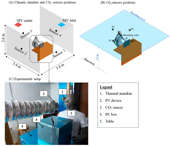
Figure 3.
Illustration of the CFD domain used for validation showing (A) the position of the sources placed at the walls, (B) the position of the sensors, and (C) the experimental setup.
4.2. Experimental Protocol
The experiment was initiated by turning ON the MV system, the lamps and the heat generated by the thermal manikin for 3 h until reaching steady-state conditions in the climatic chamber. Then, CO2 concentration naturally present in the chamber was measured before activating the CO2 sources. The obtained value will be subtracted from the total CO2 concentration measured at each point during the experiment. The CO2 sources were activated until a constant average CO2 concentration was attained in the room. After reaching steady conditions, the PV system was activated at a temperature of 23 0.2 °C and at the adequate velocity of the studied case for 3 h until the flow field and the species concentration field reaches steady-state conditions. Then, the MV system was either completely turned OFF (no current was fed to the MV supply fans) or operated at half its capacity (half the maximum current was fed to the MV fans) for 3 h according to the studied case. It is worth mentioning that during the MV malfunctioning period, the outlet fans were kept operating to balance the supply flow rate of the PV and the CO2 sources. During this period, instantaneous measurements of the CO2 concentrations were taken at the different points mentioned in Section 5.1 to monitor their buildup in the breathing zone of the manikin and in the background. Then, the supply and outlet fans were turned ON again at full capacity and instantaneous CO2 measurements were taken to observe the dilution of CO2. At each PV design flow rate and shutoff percentage of the MV system, the experiment was repeated five times to ensure repeatability and accuracy of the obtained results.
5. Results
The rate at which the CO2 level built-up and recovered, as well as the maximum attainable CO2 concentration in the macroclimate and in the occupant breathing zone, were dependent on the period and percentage of MV shutoff as well as the PV design supply flow rate. The accuracy of the developed CFD model at predicting and accurately capturing the time-dependent build-up and recovery, as well as the maximum CO2 level at different positions inside the room, was validated experimentally. Then, the validated model was used to conduct a parametric study and evaluate the resilience aspect of the combined MV–PV system with different PV design flow rates and different shock degrees.
5.1. Validation of the Developed CFD Model
The experimental conditions were simulated using the developed CFD model for the climatic chamber used for the experiment for the case of 3 h malfunctioning period and were repeated for the two different PV design flow rates of 4 L/s and 13 L/s and two different MV shutoff percentages of 100% and 50%. In this section, the CO2 concentration fields predicted by CFD are presented along with the values obtained experimentally at the breathing level (average of points P1, P2, P3, and P4) and at the breathing zone (see Figure 3B).
Figure 4 presented the CO2 contours at a horizontal plane situated at the breathing level of the manikin and showed the difference between the concentrations in the macroclimate and in the breathing zone for different shutoff percentages (100% and 50%) and PV design flow rates (4 L/s and 13 L/s). It was concluded that the average macroclimate CO2 concentration decreased from an average of 1480 82 ppm to 1300 75 ppm when the MV shutoff percentage decreased from 100% to 50% (Figure 4A,B). As for the breathing zone, it was observed that, for a MV shutoff percentage of 100%, the average CO2 concentration at the breathing zone of the manikin decreased from 1270 80 ppm to 1080 72 ppm at the end of the shock when the PV supply flow rate increased from 4 L/s to 13 L/s (Figure 4A). Similarly, for a MV shutoff percentage of 50%, the average CO2 concentration measured at the breathing zone of the manikin at the end of the shock decreased from 1180 74 ppm to 1055 80 ppm when the PV design flow rate increased from 4 L/s to 13 L/s (Figure 4B). This was due to the higher dilution effect created by the high-flow rate PV supply compared to that created by the low-flow rate PV supply.
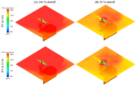
Figure 4.
CO2 concentration (ppm) contours at the horizontal plane at the breathing level of the manikin at the end of the shock for different PV design flow rates (4 L/s and 13 L/s) and different shutoff percentages of the MV system: (A) 100% and (B) 50% shutoff.
Figure 5 presented the numerical and experimental values of the temporal CO2 concentrations inside the macroclimate (which is the average of the values measured at points P1, P2, P3, and P4, see Figure 3) and at the manikin breathing zone. In the macroclimate, it was noticed that at the onset of the shock, it took 14 min for the CO2 to build up from 1100 80 ppm to 1480 82 ppm for the case of 100% shutoff, while it took 22 min to build up from 1100 80 ppm to 1300 75 ppm for the case of 50% shutoff. As for the recovery, at the end of the shock, the CO2 reached its initial values in 7 min for the case of 100% shutoff, while it took 5 min to recover for the case of 50% shutoff (Figure 5(A1,B1)).
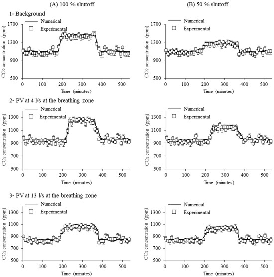
Figure 5.
Comparison of the experimental and numerical values of the CO2 concentrations in the background and in the breathing zone with PV design flow rates of 4 L/s and 13 L/s and for MV shutoff percentages of (A) 100% and (B) 50% (where the explanation for 1–3 applies to subfigures (A,B)).
As for the measurements that were taken at the breathing zone of the manikin, it was found that for a fixed degree of shock, for higher PV design flow rates, the CO2 build-up and recovery rates increased due to the larger entrainment rate. For the case of MV shutoff percentage of 100%, increasing the PV design flow rate from 4 L/s to 13 L/s decreased the time for the manikin’s breathing zone CO2 concentration to rise from the initial (950 75 ppm for PV at 4 L/s and 850 75 ppm for PV at 13 L/s) to peak values (1270 80 ppm for PV at 4 L/s and 1080 72 ppm for PV at 13 L/s) from 25 min to 20 min (Figure 5(A2,A3)). Similarly, for the case of an MV shutoff percentage of 50%, increasing the PV design flow rate from 4 L/s to 13 L/s decreased the build-up time from 33 min (from 950 75 ppm to 1180 74 ppm) to 29 min (from 850 75 ppm to 1055 80 ppm) (Figure 5(B2,B3)). Furthermore, when the shock was stopped, the peak CO2 level decreased back to their initial values at a faster rate than when the PV was designed at a higher flow rate. For the case of an MV shutoff percentage of 100%, at the end of the shock, the CO2 concentration at the manikin breathing zone reached their initial state in 20 min, and 14 min for the case of a PV designed at 4 L/s and 13 L/s, respectively (Figure 5(A2,A3)). Similarly for the case of a shutoff percentage of 50%, where the recovery time decreased from 18 min to 12 min when the PV design flow rate increased from 4 L/s to 13 L/s (Figure 5(B2,B3)).
The results showed good agreements between the numerical and experimental values of the CO2 concentration in the macroclimate and in the manikin breathing zone with the maximum relative errors as follows: 10% (100% shutoff, Background Figure 5(A1)), 7% (50% shutoff, Background Figure 5(B1)), 12% (100% shutoff, PV at 4 L/s Figure 5(A2)), 10% (50% shutoff, PV at 4 L/s Figure 5(B2)), 11% (100% shutoff, PV at 13 L/s Figure 5(A3)), and 9% (50% shutoff, PV at 13 L/s Figure 5(B3)).
5.2. Parametric Study
To study the ventilation resilience performance of the combined PV–MV system, a parametric study was conducted for two different MV malfunctioning periods (3 h and 6 h), two different MV shutoff percentages (100% and 50% shutoff), and for three different PV design flow rates (4 L/s, 9 L/s, and 13 L/s). The MV malfunctioning periods and shutoff percentages were adopted as they reflect different degrees of shocks during which the main ventilation system is either completely off (100% shutoff) or functioning at half its normal capacity (50% shutoff) for 30% (3 h) or 67% (6 h) of the total occupied time. The range of PV supply flow rates was adopted as it reflected different PV design conditions providing acceptable thermal comfort level to the occupant. In addition, the resilience of the PV–MV system was studied by considering a total shutoff of the PV devices while keeping the MV system operating at normal conditions during the entire occupied period. The aim was to evaluate the ventilation resilience of the combined PV–MV system, and the influence of the following different parameters: the PV design flow rate, the MV shutoff percentage, and the MV malfunctioning duration. The latter was investigated by monitoring the temporal variation in CO2 concentration at the occupant breathing zone for each set of conditions presented in Table 1. In addition, different aspects of resilience performance (absorptivity, recovery, and resilience indices described in Section 2.2) were determined and compared.
5.2.1. CO2 Build-Up in the Macroclimate
This sub-section studied the effect of different degrees of shock (MV malfunctioning periods and shutoff percentages) on the CO2 concentration inside the macroclimate of the office space shown in Figure 1. It is noteworthy to mention that the combined effect of MV shutoff on thermal comfort and air quality levels were not studied in this work. However, for prolonged durations of MV malfunction, the temperature in the macroclimate may increase to the point where it may jeopardize the comfort of the occupants and their perceived air quality. Hence, it was found that for the worst case scenario corresponding to a MV malfunctioning period of 6 h with a 100% shutoff (a shock degree of 0.67), the average space temperature reached 28.7 °C, indicating acceptable thermal comfort levels when combined with PV devices that supply at 23 °C [83].
The room-averaged CO2 concentrations were calculated as the volume average value of the CO2 concentrations in the space, and they showed negligible variations at the selected PV design flow rates. As presented in Figure 6, when the MV shutoff percentage increased for a fixed malfunctioning duration, the rate of CO2 build-up increased. This was due to the smaller operating flow rate of the supply and outlet MV fans during the shock leading to a reduced rate of supplied clean air and exhausted CO2-laden air from the room. In addition, when increasing the shutoff percentage, less air was supplied from the MV system resulting in less dilution of the total room air hence, a higher CO2 saturation concentration was reached at steady-state conditions. Hence, at the end of the shock, more time was needed for the higher shutoff percentage (with a higher CO2 saturation concentration) to reach back to initial CO2 values. For instance, for a malfunctioning period of 3 h (Figure 6A), the CO2 concentration increased from an initial value of 1100 ppm to a saturation value of 1520 ppm in 12 min for a 100% shutoff (corresponding to a shock degree of 0.33), whereas for a 50% shutoff (corresponding to a shock degree of 0.16), it increased to a saturation value of 1350 ppm in 20 min. At the end of the shock, the average CO2 concentration decreased back to its initial value of 1100 ppm in 7 min for the case of 100% shutoff, and in 5 min in the case of 50% shutoff. For the same MV shutoff percentage, when the shutoff period increased from 3 h to 6 h, the same build-up and recovery periods were recorded, and the saturation concentrations remained the same; however, they plateaued for a longer period of time. For the case of 100% shutoff, the saturation concentration of 1520 ppm was maintained for a duration of 168 min for the 3 h malfunction while it was maintained for 348 min in the case of 6 h shutoff (see Figure 6B). Similarly, for the case of 50% shutoff, the saturation concentration of 1350 ppm was maintained for 160 min, and 340 min when the MV was malfunctioning for a period of 3 h and 6 h, respectively.
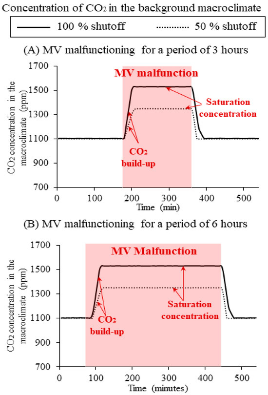
Figure 6.
The temporal variation in the CO2 concentrations in the office macroclimate for MV malfunctioning period of (A) 3 h and (B) 6 h and for shutoff percentages of 100% and 50%.
5.2.2. CO2 Build-Up in the Breathing Zone of the Occupant
In this sub-section, the CO2 concentration was monitored at the breathing zone of one occupant using the PV device. Note that similar conditions of the flow field were obtained around each of the four PV users, hence the obtained CO2 variation at the breathing zone of one occupant was considered to be representative for all of them.
- The effect of PV design flow rate
The temporal variation in the CO2 concentration at the breathing zone of one PV user was monitored in Figure 7 for different PV design flow rates associated with the MV system and different degrees of shocks. It was shown that for the same degree of shock (same MV malfunctioning period and same shutoff percentage), when the PV design supply flow rate was highest, the rate of CO2 build-up in the breathing increased, and quickly reached the 1000 ppm threshold value. This was due to the higher entrainment effect associated with higher supply velocities as follows: the elevated supply flow rate increased the velocity gradient inside the mixing layer of the jet, thus increasing the rate at which the PV jet was mixing with the room air. Another contributing factor was the greater CO2 gradient observed between the high flow rate PV jet and its surroundings, as opposed to the gradient recorded between the low flow rate PV jet and the surrounding environment. For instance, for a malfunctioning period of 3 h and a 100% shutoff (corresponding to a shock degree of 0.33) (Figure 7(A1)), at the onset of the shock, when the PV design flow rate was equal to 13 L/s, the CO2 concentration increased from an initial value of 784 ppm to 1000 ppm (threshold value) in 15 min, while it increased from the initial values of 840 ppm to 1000 ppm in 17 min for the case of PV at 9 L/s. When the PV design supply flow rate was further decreased to 4 L/s at the onset of the shock, the CO2 concentration increased from an initial value of 885 ppm to 1000 ppm in 20 min. Similar results were obtained for the case of an MV malfunctioning period of 3 h and a 50% shutoff (corresponding to a shock degree of 0.16) (Figure 7(A2)) where the build-up period from the initial CO2 concentration to the threshold value recorded 25 min, 27 min, and 30 min for the case of PV design flow rate at 13 L/s, 9 L/s, and 4 L/s, respectively.
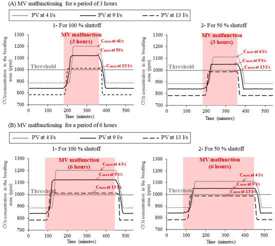
Figure 7.
The temporal variation in the CO2 concentrations in the breathing zone of the PV user for different PV design supply flow rates (4 L/s, 9 L/s, and 13 L/s) associated with the same MV system, different shutoff percentages (100% shutoff and 50% shutoff) and for an MV malfunctioning period of (A) 3 h and (B) 6 h.
Additionally, for the same degree of shock, when the PV was operated at a higher design flow rate, a better dilution at the occupant breathing zone was observed, which resulted in a lower CO2 concentration at the saturation level (). This was due to the larger distance of the PV core jet as shown in Figure 8, which presented the CO2 contours at the end of the shock in the region situated between the occupant breathing zone and the PV inlet for different degrees of shock and PV design supply flow rates. The longest core jet was observed for the case of PV supplying at 13 L/s while it eroded gradually as the design supply flow rate decreased to 9 L/s and 4 L/s. This damage in the PV core jet implied an increase in the average CO2 concentration calculated at the breathing zone of the occupant. For instance, for a MV malfunctioning period of 6 h and a 100% shutoff (corresponding to a shock degree of 0.67) (Figure 7(B1) and Figure 8A), recorded values of 1.00 ppm, 1121 ppm, and 1010 ppm for the case of a PV supplying at 4 L/s, 9 L/s, and 13 L/s. Similarly, for the case of a MV malfunctioning period of 6 h and a 50% shutoff (corresponding to a shock degree of 0.33) (Figure 7(B2) and Figure 8B), the varied between 1109 ppm for the case of PV at 4 L/s, it decreased to 1050 ppm for the case of PV at 9 L/s, and further decreased to 985 ppm for the case of PV at 13 L/s.
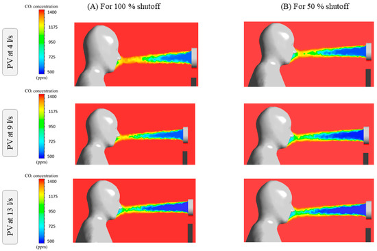
Figure 8.
CO2 concentration (ppm) contours at the occupant mid-plane at the end of the shock for different PV design flow rates (4 L/s, 9 L/s, and 13 L/s) and different shutoff percentages of the MV system: (A) 100% and (B) 50% shutoff.
Lastly, it was observed that for the same degree of shock, the time it takes for the CO2 concentration to decrease back to its initial steady-state value after the end of the shock decreased when the PV supply flow rate increased. This was due to the higher entrainment rate associated with the high PV design flow rate as well as the higher CO2 gradient between the PV jet and the surroundings. For instance, when the MV was malfunctioning for 6 h at 100% shutoff (corresponding to a shock degree of 0.67) (Figure 7(B1)) at the end of the shock, when the PV was designed at 13 L/s the CO2 concentration at the breathing zone decreased from a of 1010 ppm to the initial concentration of 784 ppm in 10 min. Similarly, for the case of a PV design at 9 L/s where the CO2 concentration decreased from 1121 ppm to 840 ppm in 12 min. Finally, for the case of a PV design at 4 L/s, it took 15 min for the CO2 concentration at the breathing zone to decrease from 1200 ppm to 885 ppm. Similar trends were observed for the case when the MV was malfunctioning for 6 h at 50% shutoff (corresponding to a shock degree of 0.33) (Figure 7(B2)) where the recovery time increased from 8 min to 10 min to 13 min for PV operating at 13 L/s, 9 L/s, and 4 L/s, respectively.
- The effect of MV shutoff percentage
The effect of the shutoff percentage on the resilience performance of the PV device was examined. The first studied case was the 100% shutoff period, which means that no air was supplied from the MV diffusers during the shock, while the second case was the 50% shutoff period meaning that during the shock, the MV was supplying air at half its normal capacity. It was shown that for a fixed-PV design supply flow rate and a fixed malfunctioning period, the rate of CO2 build-up decreased when the shutoff percentage decreased. This was due to the lower CO2 concentration gradient between the PV jet and the surroundings, and the lower CO2 build-up rate at the background level, as explained in Section 5.2.1, leading to a slower entrainment. For instance, for a PV design flow rate of 9 L/s and a malfunctioning period of 3 h at the onset of shock, the CO2 concentration increased from an initial concentration of 840 ppm to the threshold value of 1000 ppm in 15 min for the case of a 100% shutoff (corresponding to a shock degree of 0.33) (Figure 7(A1)), while it increased in 25 min for the case of a 50% shutoff (corresponding to a shock degree of 0.16) (Figure 7(A2)). Similar build-up periods were obtained for the case of a malfunctioning period of 6 h (Figure 7B). In addition, the lower shutoff percentage resulted in a reduced since it coincided with a lower background CO2 concentration, as shown in Figure 4. For instance, for a shutoff period of 6 h, and a PV design flow rate of 9 L/s, decreased from 1121 ppm to 1050 ppm when the shutoff percentage decreased from 100% (corresponding to a shock degree of 0.67) (Figure 7(B1) and Figure 8A—PV at 9 L/s) to 50% (corresponding to a shock degree of 0.33) (Figure 7(B2) and Figure 8B—PV at 9 L/s).
Finally, the time during which the CO2 concentration goes back from to the initial steady-state values decreased when the shutoff percentage decreased. In fact, when the shutoff percentage decreased, the rate of recovery for the background surroundings increased, as explained in Section 5.2.1, which resulted in an increased entrainment rate into the PV jet. For example, for a PV design flow rate of 9 L/s and a malfunctioning period of 6 h at the end of shock, the CO2 concentration decreased from of 1121 ppm to the initial steady-state concentration of 840 ppm in 12 min for the case of a 100% shutoff (corresponding to a shock degree of 0.67) (Figure 7(B1)), while it decreased in 10 min for the case of a 50% shutoff (corresponding to a shock degree of 0.33) (Figure 7(B2)).
- The effect of MV malfunctioning duration
The effect of the MV malfunctioning duration (6 h and 3 h) on the resilience performance of the PV device was investigated. It was observed that, for the same PV flow rate design and same MV shutoff percentage, when the shutoff period increased, the trend of temporal CO2 variation in the breathing zone remained the same (same rate of CO2 build-up and recovery). It was shown in Figure 7A,B that the duration of CO2 build-up in the breathing zone was in the order of minutes for all the design PV flow rates and shutoff percentages, which means that was attained for both the 3 h and 6 h malfunction period; however, for the case of longer malfunctioning periods, plateaued for a longer period of time. For instance, for a PV design flow rate of 9 L/s and a shutoff percentage of 100%, (1121 ppm: 121 ppm higher than the recommended CO2 threshold concentration) plateaued for 163 min when the malfunctioning period was 3 h (corresponding to a shock degree of 0.33) while it plateaued for 343 min for a malfunctioning period of 6 h (corresponding to a shock degree of 0.67) (Figure 7(A1,B1)). Similarly, for a PV design flow rate of 9 L/s and a shutoff percentage of 50 %, (1050 ppm: 50 ppm higher than the recommended CO2 threshold concentration) plateaued for 153 min when the malfunctioning period was 3 h (corresponding to a shock degree of 0.16), while it plateaued for 333 min for a malfunctioning period of 6 h (corresponding to a shock degree of 0.33) (Figure 7(A2,B2)). Similar trends were observed for the remaining PV design flow rates.
5.2.3. Assessment of the Different Aspects of the PV Ventilation Resilience
To investigate the different resilience responses of the PV device for different design supply flow rates for the same MV system, MV malfunctioning periods, and shutoff percentages, the three resilience aspects were calculated at each set of parameters and presented in the form of spider charts in Figure 9 and summarized in Table 3. It was shown that for a fixed degree of shock, for a higher PV design supply flow rate, decreased, increased, and increased, indicating a fast absorption of the shock, a fast recovery at the end of the shock, and a low shock impact, respectively. For example, when the MV was malfunctioning for 6 h at a shutoff percentage of 100% (corresponding to a shock degree of 0.67), decreased gradually from 0.027 to 0.019 to 0.011 when the PV design supply flow rate increased from 4 L/s to 9 L/s to 13 L/s, respectively (Figure 9(B1)). As for , it increased gradually from 0.953 to 0.972 to 0.981 when the PV design supply flow rate was increased from 4 L/s to 9 L/s to 13 L/s, respectively. Finally, increased from 0.61 to 0.80 to 0.97 when the PV design supply flow rate increased from 4 L/s to 9 L/s to 13 L/s, respectively. The same trends were observed for the remaining shock degrees. However, it is noteworthy to mention the curve of the PV at 13 L/s was omitted from the spider chart for the case of 50% shutoff (Figure 9(A2,B2)), since under those conditions the CO2 concentration at the breathing zone of the occupant did not surpass the threshold value of 1000 ppm (Figure 8B—PV at 13 L/s), hence they had a resilience effectiveness equal to 1. Those indices were calculated [45] to evaluate the ventilation resilience (build-up of CO2) of constant air volume ventilation system in a large classroom at different mechanical shocks. They found that was varying between 0.15 and 0.55 and was varying between 0.62 and 0.92. These values were higher than those obtained for the case of MV–PV resilience. This was explained as follows: the targeted zone in case of the PV is the breathing zone, while in the case of the constant air volume system, it is the entire classroom having the dimensions of 13.28 m length 10.69 m width 2.7 m height. Hence, more time was needed to build-up the CO2 levels to above their threshold limits and more time is needed to dilute the CO2 to its initial values below the threshold limit. Furthermore, varied between 0.25 and 0.98 in the case of classroom ventilated by a constant air volume system compared to a variation between 0.61 and 1.0 in the case of a combined MV–PV system in an office space. This increase was due to the elevated number of occupants generating CO2 in the classroom compared to only four occupants in the office space. In addition, during a MV malfunction, the clean air of the PV devices mixes with the entrained CO2-laden air, resulting in a reduction in the CO2 level at the breathing zone compared to those observed in the macroclimate. Consequently, lower ppm·hours were observed in the case of combined PV–MV resilience compared to the constant air volume resilience, leading to a lower resilience level (lower ).
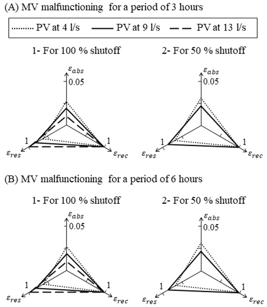
Figure 9.
Spider charts showing the three aspects of ventilation resilience () for different PV design supply flow rates (4 L/s, 9 L/s, and 13 L/s), shutoff percentages (100% and 50% shutoff), and MV malfunctioning periods of (A) 3 h and (B) 6 h.
Table 3.
Values of absorptivity (), recovery (), and resilience () effectiveness for different PV design flow rates (4 L/s, 9 L/s, and 13 L/s), shutoff percentages (50% and 100%), and malfunctioning periods (3 h and 6 h).
For the case when the PV design flow rate and the MV malfunctioning period were fixed, when the shutoff percentage was decreased, increased, increased, and increased, indicating a gradual absorption of the shock, a fast recovery at the end of the shock and a low shock impact, respectively. Decreasing the shutoff percentage resulted in (1) shorter periods above the recommended CO2 threshold limit and (2) lower CO2 concentrations values (Figure 7(B1,B2)). For example, for a PV design supply flow rate of 9 L/s and a malfunctioning period of 6 h, when the shutoff percentage decreased from 100% (corresponding to a shock degree of 0.67) (Figure 9(B1)) to 50% (corresponding to a shock degree of 0.33), (Figure 9(B2)) increased from 0.019 to 0.022, increased from 0.972 to 0.985, and increased from 0.80 to 0.85.
For the case when the PV design flow rate and the MV shutoff percentage were fixed, when the malfunctioning period increased, remained the same, remained the same, and decreased, indicating a higher shock impact. Increasing the time of MV malfunction prolonged the hours during which was maintained at the breathing zone of the occupant, thus leading to a higher shock impact. For instance, for a PV design supply flow rate of 9 L/s and a shutoff percentage of 100%, when the malfunction period increased from 3 h (corresponding to a shock degree of 0.33) (Figure 9(A1)) to 6 h (corresponding to a shock degree of 0.67) (Figure 9(B1)) was maintained to 0.019, was maintained to 0.972 while decreased from 0.81 to 0.80. Similar trends were observed for all the PV design flow rate and shutoff percentages.
5.2.4. Shutoff of the PV System
To evaluate the resilience of the MV + PV system, the case when the PV device was turned OFF was evaluated. In this case, the MV system was operating at its full capacity during the entire occupied period, while the PV devices were turned OFF for 2 min. The temporal variation in CO2 concentrations was monitored in Figure 10 at the breathing zone of the occupant for PV design supply flow rates of 4 L/s, 9 L/s, and 13 L/s. It was determined that the rate of build-up and recovery of CO2 at the occupant breathing zone was fast in the case of PV turned OFF. This was due to the fact that the fresh air supplied by the PV devices was oriented directly toward the face of the user. Hence, the targeted zone was situated at a short distance from the PV supply opening, which issued the fresh air at a high momentum (0.5 m/s for the case of PV supplying at 4 L/s, and 1.7 m/s for the case of PV supplying at 13 L/s).
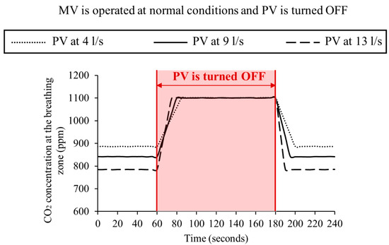
Figure 10.
Temporal variation in CO2 concentration (ppm) in the breathing zone of the occupant for the case when the MV is normally operated while the PV devices are shutoff for 2 min and for different PV design supply flow rate (4 L/s, 9 L/s, and 13 L/s).
At the onset of PV shutoff, as the PV design supply flow rate increased, the CO2 build-up rate increased, which was due the larger gradient of CO2 concentration between the breathing zone and the macroclimate. For instance, the build-up period decreased from 16 s to 14 s to 10 s when the PV design flow rate was increased from 4 L/s to 9 L/s to 13 L/s. After building-up, the CO2 concentration at the breathing zone plateaued at a value equal to that of the average CO2 concentration in the macroclimate (1100 ppm). In addition, at the end of the PV shutoff, as the PV design supply flow rate increased, the recovery time decreased, which was due to the faster supply of fresh air. For example, the recovery time decreased from 13 s to 11 s to 7 s when the PV design flow rate was increased from 4 L/s to 9 L/s to 13 L/s.
6. Limitations and Applicability
This study investigated the ventilation resilience of the combined PV–MV system in a typical office space. In particular, it focused on the CO2 build-up in the macroclimate, and in the occupant breathing zone resulting from a sudden malfunction of the MV system or the PV devices. However, in addition to their effect on the quality of breathable air, these malfunctions may have additional consequences, such as the undesirable temperature build-up, which may compromise the thermal comfort of the occupants. Therefore, the combined effect of sudden MV and PV malfunctions on both thermal comfort and CO2 build-up can be studied in future works for a more holistic understanding of the challenges posed by the ventilation system disruptions.
7. Conclusions
This work studies the ventilation resilience of the combined PV–MV system when operating in an office space containing four occupants. Mechanical shocks, which consider the malfunction of the MV system on one hand, and the total shutoff of the PV devices on the other hand, were studied. The malfunction of the MV system accounted for a complete (100%) and a partial (50%) shutoff of the MV system at two different durations (6 h and 3 h) and for three different operation designs of the PV (4 L/s, 9 L/s, and 13 L/s). The shutoff of the PV devices was also studied to account for any sudden failure of the PV own air handling unit. A 3D CFD model was developed for this aim and validated experimentally in a controlled climatic chamber. For each combination of PV design flow rates, shock durations, and shutoff periods, three aspects of resilience behavior were calculated to quantify the absorption () and recovery capacity () of the PV devices, as well as the shock impact (). The following conclusions were drawn:
- Concerning the build-up of CO2 in the macroclimate, the results showed that when decreasing the shutoff percentage from 100% to 50%, the following lower CO2 saturation concentrations were reached: 1520 ppm for the case of 100% shutoff and 1350 ppm for the case of 50% shutoff. Additionally, the CO2 build-up period increased from 12 min to 20 min. However, the recovery period decreased from 7 min to 5 min;
- Concerning the CO2 build-up in the breathing zone of the occupant, it was showed that for a fixed degree of shock, using a higher PV design supply flow rate resulted in a fast absorption of the shock, a fast recovery at the end of the shock due to the higher entrainment rate, and a low shock impact due to the lower ;
- It was recommended to design the PV devices at a flow rate not less than 13 L/s for better resilience effectiveness. This operation resulted in a resilience effectiveness equal to 1 for the case of a 50% shutoff and values close to unity for the case of a 100% shutoff;
- When decreasing the shutoff percentage of the MV system, the CO2 saturation concentration at the breathing zone of the occupant decreased and plateaued for a shorter period of time for the same malfunction duration, which resulted in a higher resilience effectiveness of the system;
- When the malfunctioning duration of the MV system showed an increase in and , the PV system remained unchanged; however, .plateaued for a longer period of time, thus resulting in lower values of ;
- The rate of build-up and recovery of CO2 at the occupant breathing zone was fast (in the range of seconds) in the case of a sudden PV shutoff. It was recommended to design the PV devices with regular maintenance and filter changes;
- Future studies should elaborate the combined effect of sudden MV and PV malfunction on both thermal comfort and CO2 build-up. It would also be interesting to investigate using PV as a backup to the MV system in case of heat wave events, when the MV system fails at maintaining the required indoor temperature, impacting occupant comfort.
Author Contributions
Conceptualization, K.G. and N.G.; formal analysis, J.K. and K.G.; methodology, K.G. and N.G.; project administration, N.G.; resources, N.G.; software, J.K.; supervision, N.G.; validation, J.K.; writing—original draft, J.K.; writing—review and editing, N.G. All authors have read and agreed to the published version of the manuscript.
Funding
This research was funded by of the American University of Beirut, Lebanon—University Research Board.
Data Availability Statement
The raw data presented and supporting the conclusions of this article will be made available by the authors upon request.
Conflicts of Interest
The authors declare no conflicts of interest. The funders had no role in the design of the study; in the collection, analyses, or interpretation of data; in the writing of the manuscript; or in the decision to publish the results.
Nomenclature
| AC | Air conditioning |
| CFD | Computational fluid dynamics |
| Cmax | Maximum concentration (ppm) |
| ∆tabs | Absorptivity time (h) |
| ∆trec | Recovery time (h) |
| εabs | Absorptivity effectiveness (-) |
| εrec | Recovery effectiveness (-) |
| εres | Resilience effectiveness (-) |
| IAQ | Indoor air quality |
| MV | Mixing ventilation |
| PV | Personalized ventilation |
| t | Time (h) |
| tocc | Occupied period (h) |
| VOC | Volatile organic compounds |
| Greek Symbols | |
| ε | Effectiveness |
| Δ | Difference |
| Subscripts | |
| abs | Absorptivity |
| occ | Occupied |
| rec | Recovery |
| res | Resilience |
References
- Arif, M.; Katafygiotou, M.; Mazroei, A.; Kaushik, A.; Elsarrag, E. Impact of indoor environmental quality on occupant well-being and comfort: A review of the literature. Int. J. Sustain. Built Environ. 2016, 5, 1–11. [Google Scholar]
- Persily, A.; Emmerich, S. Indoor Environmental Resilience: A Review and Discussion. In Proceedings of the Healthy Buildings 2015 America, Innovation in a Time of Energy Uncertainty and Climate Adaptation, Boulder, CO, USA, 19–22 July 2015. [Google Scholar]
- Persily, A.K.; Emmerich, S.J. Indoor Environmental Issues in Disaster Resilience; US Department of Commerce, National Institute of Standards and Technology: Gaithersburg, MD, USA, 2015.
- Anand, P.; Sekhar, C.; Cheong, D.; Santamouris, M.; Kondepudi, S. Occupancy-based zone-level VAV system control implications on thermal comfort, ventilation, indoor air quality and building energy efficiency. Energy Build. 2019, 204, 109473. [Google Scholar] [CrossRef]
- Harčárová, K.; Vilčeková, S. Indoor environmental quality in green certified office buildings. IOP Conf. Ser. Mater. Sci. Eng. 2022, 1252, 012054. [Google Scholar] [CrossRef]
- Abdullah, H.K.; Alibaba, H.Z. Window design of naturally ventilated offices in the mediterranean climate in terms of CO2 and thermal comfort performance. Sustainability 2020, 12, 473. [Google Scholar] [CrossRef]
- Saheb, H.; Mahdi, A.; Al-amir, Q. A numerical and experimental study of the effect of using personal ventilation systems on indoor air quality in office rooms. Front. Heat Mass Transf. 2021, 16, 9. [Google Scholar] [CrossRef]
- Zhou, J.; Kim, C.N. Effect of the personalized ventilation on indoor air quality for an indoor occupant with VOCs emission from carpet. J. Mech. Sci. Technol. 2012, 26, 481–488. [Google Scholar] [CrossRef]
- Melikov, A.K.; Cermak, R.; Majer, M. Personalized ventilation: Evaluation of different air terminal devices. Energy Build. 2002, 34, 829–836. [Google Scholar] [CrossRef]
- Song, W.; Zhang, Z.; Chen, Z.; Wang, F.; Yang, B. Thermal comfort and energy performance of personal comfort systems (PCS): A systematic review and meta-analysis. Energy Build. 2022, 256, 111747. [Google Scholar] [CrossRef]
- Schiavon, S.; Melikov, A.K.; Sekhar, C. Energy analysis of the personalized ventilation system in hot and humid climates. Energy Build. 2010, 42, 699–707. [Google Scholar] [CrossRef]
- Rawal, R.; Schweiker, M.; Kazanci, O.B.; Vardhan, V.; Jin, Q.; Duanmu, L. Personal comfort systems: A review on comfort, energy, and economics. Energy Build. 2020, 214, 109858. [Google Scholar] [CrossRef]
- Cermak, R.; Melikov, A.K.; Forejt, L.; Kovar, O. Performance of personalized ventilation in conjunction with mixing and displacement ventilation. Hvac&R Res. 2006, 12, 295–311. [Google Scholar]
- Yang, B.; Liu, Y.; Zhu, X.; Li, X. Personalized Ventilation Systems. In Personal Comfort Systems for Improving Indoor Thermal Comfort and Air Quality; Springer: Berlin/Heidelberg, Germany, 2023; pp. 113–127. [Google Scholar]
- Pantelic, J.; Tham, K.W.; Licina, D. Effectiveness of a personalized ventilation system in reducing personal exposure against directly released simulated cough droplets. Indoor Air 2015, 25, 683–693. [Google Scholar] [CrossRef]
- Shinoda, J.; Bogatu, D.-I.; Watanabe, F.; Kaneko, Y.; Olesen, B.W.; Kazanci, O.B. Performance evaluation of a multi-functional personalized environmental control system (PECS) prototype. Build. Environ. 2024, 252, 111260. [Google Scholar] [CrossRef]
- Saheb, H.A.; Al-amir, Q.R. A Comparative Study of Performance Between Two Combined Ventilation Systems and Their Effect On Indoor Air Quality and Thermal Comfort Inside Office Rooms. IOP Conf. Ser. Mater. Sci. Eng. 2021, 1095, 012001. [Google Scholar] [CrossRef]
- Xu, J.; Wang, C.; Fu, S.; Chan, K.; Chao, C.Y. Short-range bioaerosol deposition and inhalation of cough droplets and performance of personalized ventilation. Aerosol Sci. Technol. 2021, 55, 474–485. [Google Scholar] [CrossRef]
- Rajput, M.; Augenbroe, G.; Stone, B.; Georgescu, M.; Broadbent, A.; Krayenhoff, S.; Mallen, E. Heat exposure during a power outage: A simulation study of residences across the metro Phoenix area. Energy Build. 2022, 259, 111605. [Google Scholar] [CrossRef]
- Chen, Y.; Lin, G.; Crowe, E.; Granderson, J. Development of a unified taxonomy for hvac system faults. Energies 2021, 14, 5581. [Google Scholar] [CrossRef]
- Mills, E. Electric Grid Disruptions and Extreme Weather; Lawrence Berkeley National Laboratory: Berkeley, CA, USA, 2012.
- Al Assaad, D.; Sengupta, A.; Breesch, H. Demand-controlled ventilation in educational buildings: Energy efficient but is it resilient? Build. Environ. 2022, 226, 109778. [Google Scholar] [CrossRef]
- Zhao, Y.; Wen, J.; Xiao, F.; Yang, X.; Wang, S. Diagnostic Bayesian networks for diagnosing air handling units faults—Part I: Faults in dampers, fans, filters and sensors. Appl. Therm. Eng. 2017, 111, 1272–1286. [Google Scholar] [CrossRef]
- Liévanos, R.S.; Horne, C. Unequal resilience: The duration of electricity outages. Energy Policy 2017, 108, 201–211. [Google Scholar] [CrossRef]
- Al Assaad, D.; Breesch, H. Evaluation of “Ventilation Resilience” in Mid-Sized Office Buildings. In Proceedings of the CLIMA 2022 Conference, Rotterdam, The Netherlands, 22–25 May 2022. [Google Scholar]
- Kalmár, F.; Kalmár, T. Alternative personalized ventilation. Energy Build. 2013, 65, 37–44. [Google Scholar] [CrossRef]
- Katramiz, E.; Al Assaad, D.; Ghaddar, N.; Ghali, K. The effect of human breathing on the effectiveness of intermittent personalized ventilation coupled with mixing ventilation. Build. Environ. 2020, 174, 106755. [Google Scholar] [CrossRef]
- Harrouz, J.P.; Karam, J.; Ghali, K.; Ghaddar, N. Personalized ventilation with embedded air treatment system for simultaneous cooling and sorption-based carbon and humidity capture. Energy Convers. Manag. 2023, 291, 117290. [Google Scholar] [CrossRef]
- Xu, C.; Wei, X.; Liu, L.; Su, L.; Liu, W.; Wang, Y.; Nielsen, P.V. Effects of personalized ventilation interventions on airborne infection risk and transmission between occupants. Build. Environ. 2020, 180, 107008. [Google Scholar] [CrossRef] [PubMed]
- Liu, W.; Liu, L.; Xu, C.; Fu, L.; Wang, Y.; Nielsen, P.V.; Zhang, C. Exploring the potentials of personalized ventilation in mitigating airborne infection risk for two closely ranged occupants with different risk assessment models. Energy Build. 2021, 253, 111531. [Google Scholar] [CrossRef] [PubMed]
- Ono, E.; Mihara, K.; Lam, K.P.; Chong, A. The effects of a mismatch between thermal comfort modeling and HVAC controls from an occupancy perspective. Build. Environ. 2022, 220, 109255. [Google Scholar] [CrossRef]
- Liu, S.; Koupriyanov, M.; Paskaruk, D.; Fediuk, G.; Chen, Q. Investigation of airborne particle exposure in an office with mixing and displacement ventilation. Sustain. Cities Soc. 2022, 79, 103718. [Google Scholar] [CrossRef] [PubMed]
- Burkett, A. Conference Room Space Planning Guideline for 2023. Available online: https://www.iofficecorp.com/blog/conference-room-space-planning (accessed on 30 November 2023).
- Alsaad, H.; Voelker, C. Performance assessment of a ductless personalized ventilation system using a validated CFD model. J. Build. Perform. Simul. 2018, 11, 689–704. [Google Scholar] [CrossRef]
- Alsaad, H.; Voelker, C. Could the ductless personalized ventilation be an alternative to the regular ducted personalized ventilation? Indoor Air 2021, 31, 99–111. [Google Scholar] [CrossRef]
- Melikov, A.K. Personalized ventilation. Indoor Air 2004, 14, 157–167. [Google Scholar] [CrossRef]
- Zeng, Q.; Zhao, R. Prediction of perceived air quality for personalized ventilation systems. Tsinghua Sci. Technol. 2005, 10, 227–232. [Google Scholar] [CrossRef]
- Russo, J.S.; Khalifa, E. Computational study of breathing methods for inhalation exposure. HVACR Res. 2011, 17, 419–431. [Google Scholar] [CrossRef]
- Melikov, A.K.; Arakelian, R.S.; Halkjaer, L.; Fanger, P.O. Spot Cooling. Part 2: Recommendations for Design of Spot-Cooling Systems. In Proceedings of the 1994 Annual Meeting of American Society of Heating, Refrigerating, and Air Conditioning Engineers (ASHRAE), Orlando, FL, USA, 25–29 June 1994; pp. 0001–2505. [Google Scholar]
- Chen, Y.; Raphael, B.; Sekhar, S. Individual control of a personalized ventilation system integrated with an ambient mixing ventilation system. HVACR Res. 2012, 18, 1136–1152. [Google Scholar] [CrossRef]
- Kaczmarczyk, J.; Melikov, A.; Fanger, P.O. Human response to personalized ventilation and mixing ventilation. Indoor Air 2004, 14, 17–29. [Google Scholar] [CrossRef] [PubMed]
- Tham, K.W.; Pantelic, J. Performance evaluation of the coupling of a desktop personalized ventilation air terminal device and desk mounted fans. Build. Environ. 2010, 45, 1941–1950. [Google Scholar] [CrossRef]
- Chen, Y.; Sekhar, C.; Tham, K.W.; Raphael, B. Personalized Ventilation Control: Perception of Indoor air Quality. In Proceedings of the 10th REHVA World Congress, Antalya, Turkey, 9–12 May 2010. [Google Scholar]
- Sekhar, S.; Gong, N.; Tham, K.W.; Cheong, K.; Melikov, A.K.; Wyon, D.; Fanger, P.O. Findings of personalized ventilation studies in a hot and humid climate. HVACR Res. 2005, 11, 603–620. [Google Scholar] [CrossRef]
- Al Assaad, D.; Sengupta, A.; Breesch, H. A novel quantitative assessment framework of the IAQ resilience performance of buildings: The resilience score metric. Build. Environ. 2023, 243, 110669. [Google Scholar] [CrossRef]
- Al-Assad, D.; Ghali, K.; Ghaddar, N. Performance of Intermittent Personalized Ventilation Assisting Mixing Ventilation in the Presence of Indoor Disturbance. In Proceedings of the Heat Transfer Summer Conference, Bellevue, DC, USA, 13–17 July 2019; p. V001T003A002. [Google Scholar]
- ANSI/ASHRAE Standard 62.1-2007; Ventilation for Acceptable Indoor Air Quality. American Society of Heating, Refrigerating and Air-Conditioning Engineers, Inc.: Atlanta, GA, USA, 2007.
- Mayer, A.J.; Menges, C.; Göttig, R. A Method for Determining the Time-Dependent Indoor CO2 Concentration to Evaluate Air Hygiene. In Proceedings of the Healthy Buildings 2021, Virtual, 21–23 June 2021. [Google Scholar]
- Zhuang, R.; Li, X.; Tu, J. CFD Study of the Effects of Furniture Layout on Indoor Air Quality under Typical Office Ventilation Schemes. In Building Simulation; Springer: Berlin/Heidelberg, Germany, 2014; pp. 263–275. [Google Scholar]
- Zhang, H.; Zhang, W.; Zhang, W.; Xuan, Y.; Yue, Y. Multi-vent module-based adaptive ventilation to reduce cross-contamination among indoor occupants. Build. Environ. 2022, 212, 108836. [Google Scholar] [CrossRef]
- Alsaad, H.; Voelker, C. CFD Analysis of Indoor Air Quality in Office Rooms Equipped with Desk Fans. In Proceedings of the Building Simulation 2019, Rome, Italy, 2–4 September 2019. [Google Scholar]
- Wu, J.; Xu, L.; Shen, J. Research on the cross-contamination in the confined conference room with the radiant floor heating system integrated with the down-supply ventilation. Heliyon 2023, 9, e14389. [Google Scholar]
- Ahmadzadeh, M.; Shams, M. A numerical approach for preventing the dispersion of infectious disease in a meeting room. Sci. Rep. 2022, 12, 16959. [Google Scholar] [CrossRef]
- Zhang, Y.; Feng, G.; Kang, Z.; Bi, Y.; Cai, Y. Numerical simulation of coughed droplets in conference room. Procedia Eng. 2017, 205, 302–308. [Google Scholar] [CrossRef]
- Abuhegazy, M.; Talaat, K.; Anderoglu, O.; Poroseva, S.V. Numerical investigation of aerosol transport in a classroom with relevance to COVID-19. Phys. Fluids 2020, 32, 103311. [Google Scholar] [CrossRef]
- Karam, J.; Ghali, K.; Ghaddar, N. Pulsating jet ventilation add-ons performance for reducing the contaminant spread in classrooms: Portable air cleaners vs. upper room UVGI. Build. Environ. 2023, 229, 109946. [Google Scholar] [CrossRef]
- Mirzaie, M.; Lakzian, E.; Khan, A.; Warkiani, M.E.; Mahian, O.; Ahmadi, G. COVID-19 spread in a classroom equipped with partition–A CFD approach. J. Hazard. Mater. 2021, 420, 126587. [Google Scholar] [CrossRef] [PubMed]
- Fluent, A. 19.2 User’s Guide; ANSYS. Inc.: Canonsburg, PA, USA, 2013. [Google Scholar]
- Abou Hweij, W.; Ghaddar, N.; Ghali, K.; Habchi, C. Optimized performance of displacement ventilation aided with chair fans for comfort and indoor air quality. Energy Build. 2016, 127, 907–919. [Google Scholar] [CrossRef]
- Lee, M.; Park, G.; Park, C.; Kim, C. Improvement of grid independence test for computational fluid dynamics model of building based on grid resolution. Adv. Civ. Eng. 2020, 2020, 8827936. [Google Scholar] [CrossRef]
- Moukalled, F.; Mangani, L.; Darwish, M.; Moukalled, F.; Mangani, L.; Darwish, M. The Finite Volume Method; Springer: Berlin/Heidelberg, Germany, 2016. [Google Scholar]
- Chen, Q.; Zhang, Z.; Zuo, W. Computational Fluid Dynamics for Indoor Environment Modeling: Past, Present and Future. In Proceedings of the XXV Congresso della Trasmissione del Calore UIT, Trieste, Italy, 18–20 June 2007. [Google Scholar]
- Zhang, Z.; Chen, Q. Comparison of the Eulerian and Lagrangian methods for predicting particle transport in enclosed spaces. Atmos. Environ. 2007, 41, 5236–5248. [Google Scholar] [CrossRef]
- Teodosiu, R.; David, D.; Teodosiu, C.; Rusaouën, G.; Ilie, V.; Nguyen, C.-K. Experimental and numerical investigation of mechanically ventilated rooms. Energy Procedia 2017, 112, 252–260. [Google Scholar] [CrossRef]
- Buratti, C.; Palladino, D.; Moretti, E. Prediction of indoor conditions and thermal comfort using CFD simulations: A case study based on experimental data. Energy Procedia 2017, 126, 115–122. [Google Scholar] [CrossRef]
- Rong, L.; Nielsen, P.V.; Bjerg, B.; Zhang, G. Summary of best guidelines and validation of CFD modeling in livestock buildings to ensure prediction quality. Comput. Electron. Agric. 2016, 121, 180–190. [Google Scholar] [CrossRef]
- Lau, J.; Niu, J. Measurement and CFD simulation of the temperature stratification in an atrium using a floor level air supply method. Indoor Built Environ. 2003, 12, 265–280. [Google Scholar] [CrossRef]
- Du, L.; Yang, C.; Dominy, R.; Yang, L.; Hu, C.; Du, H.; Li, Q.; Yu, C.; Xie, L.; Jiang, X. Computational Fluid Dynamics aided investigation and optimization of a tunnel-ventilated poultry house in China. Comput. Electron. Agric. 2019, 159, 1–15. [Google Scholar] [CrossRef]
- Wang, C.; Liu, J.; Li, J.; Li, F. Chaotic behavior of human thermal plumes in an aircraft cabin mockup. Int. J. Heat Mass Transf. 2018, 119, 223–235. [Google Scholar] [CrossRef]
- Wang, C.; Liu, J.; Li, J. Mini-PIV Determination of Unsteady Characteristic of Human Thermal Plume. In Proceedings of the 10th International Symposium on Heating, Ventilation and Air Conditioning—ISHVAC 2017, Jinan, China, 19–22 October 2017. [Google Scholar]
- Sahebl, H.A.; Al-amir, Q.R. CFD Analysis for The Effect of Personal Ventilation Combined with Mixing Ventilation on Performance Index (ADPI) and Thermal Human Comfort. IOP Conf. Ser. Mater. Sci. Eng. 2020, 978, 012033. [Google Scholar] [CrossRef]
- Ray, S.D.; Gong, N.-W.; Glicksman, L.R.; Paradiso, J.A. Experimental characterization of full-scale naturally ventilated atrium and validation of CFD simulations. Energy Build. 2014, 69, 285–291. [Google Scholar] [CrossRef]
- Song, J.; Meng, X. The improvement of ventilation design in school buildings using CFD simulation. Procedia Eng. 2015, 121, 1475–1481. [Google Scholar] [CrossRef]
- Al Assaad, D.; Ghali, K.; Ghaddar, N.; Habchi, C. Mixing ventilation coupled with personalized sinusoidal ventilation: Optimal frequency and flow rate for acceptable air quality. Energy Build. 2017, 154, 569–580. [Google Scholar] [CrossRef]
- Thermetrics. Newton Thermal Mannikin System. Available online: https://www.thermetrics.com/products/full-body-manikins/newton (accessed on 1 December 2023).
- Kulkarni, V.; Sahoo, N.; Chavan, S.D. Simulation of honeycomb–screen combinations for turbulence management in a subsonic wind tunnel. J. Wind Eng. Ind. Aerodyn. 2011, 99, 37–45. [Google Scholar] [CrossRef]
- Karam, J.; Katramiz, E.; Ghali, K.; Ghaddar, N. Effective mitigation of cross-contamination in classroom conditioned by intermittent air jet cooling with use of portable air cleaners. Build. Environ. 2022, 219, 109220. [Google Scholar] [CrossRef]
- Shokrollahi, S.; Hadavi, M.; Heidarinejad, G.; Pasdarshahri, H. Multi-objective optimization of underfloor air distribution (UFAD) systems performance in a densely occupied environment: A combination of numerical simulation and Taguchi algorithm. J. Build. Eng. 2020, 32, 101495. [Google Scholar] [CrossRef]
- Mahyuddin, N.; Awbi, H. The spatial distribution of carbon dioxide in an environmental test chamber. Build. Environ. 2010, 45, 1993–2001. [Google Scholar] [CrossRef]
- Chakroun, W.; Ghali, K.; Ghaddar, N. Air quality in rooms conditioned by chilled ceiling and mixed displacement ventilation for energy saving. Energy Build. 2011, 43, 2684–2695. [Google Scholar] [CrossRef]
- CO2Meter. Available online: https://www.co2meter.com/collections/5-percent-co2-sensor (accessed on 30 October 2023).
- SWEMA03. Available online: https://swema.com/product/swema-03/ (accessed on 31 August 2023).
- Itani, M.; Ghaddar, D.; Ghaddar, N.; Ghali, K. Model-based multivariable regression model for thermal comfort in naturally ventilated spaces with personalized ventilation. J. Build. Perform. Simul. 2021, 14, 78–93. [Google Scholar] [CrossRef]
Disclaimer/Publisher’s Note: The statements, opinions and data contained in all publications are solely those of the individual author(s) and contributor(s) and not of MDPI and/or the editor(s). MDPI and/or the editor(s) disclaim responsibility for any injury to people or property resulting from any ideas, methods, instructions or products referred to in the content. |
© 2024 by the authors. Licensee MDPI, Basel, Switzerland. This article is an open access article distributed under the terms and conditions of the Creative Commons Attribution (CC BY) license (https://creativecommons.org/licenses/by/4.0/).