
FBG-Based Accelerometer for Buried Pipeline Natural Frequency Monitoring and Corrosion Detection

 ,
,  ,
,  , ,
, ,  ,
,  ,
,  and
and 
Abstract
1. Introduction

| Techniques | Advantages | Disadvantages | Reference |
|---|---|---|---|
| Visual inspection | Cheap and easy method | Difficult to detect corrosion in early stages and in difficult access areas | [30] |
| Ultrasound | Widely disseminated method with high precision | Measurements conducted in small regions and time-consuming process | [11] |
| Ultrasonic guided waves (UGW) | Able to assess corrosion over long distances in large structures (e.g., pipelines) | External actions can cause a considerable influence that can lead to false indications of defects | [15] |
| Ground Penetration Radar (GPR)—single-polarization system | Able to indicate damage in buried pipelines | Restricted information regarding corrosion products (e.g., rust and cracks) | [18] |
| Ground Penetration Radar (GPR)—hybrid-polarization system | Able to detect corrosion products (e.g., rust and cracks) | Does not perform quantitative assessment | [19] |
| Radiography | Identification of variations in the thickness of 10%, 20%, and 50% | Measurements conducted in small regions and time-consuming process | [23] |
| Eddy current | Widely disseminated method especially applied for access surface damage | Only applied for unburied pipelines | [26] |
| Thermography | Able to detect the reduction in the metal thickness | In case of corrosion detection in buried pipelines, it may be necessary to analyze the soil characteristics | [29] |
| Galvanic sensors | Able to quantify the corrosion in metallic elements | Susceptible to aggressive environments | [31] |
2. Materials and Methods
2.1. Fiber Bragg Gratings
- i.
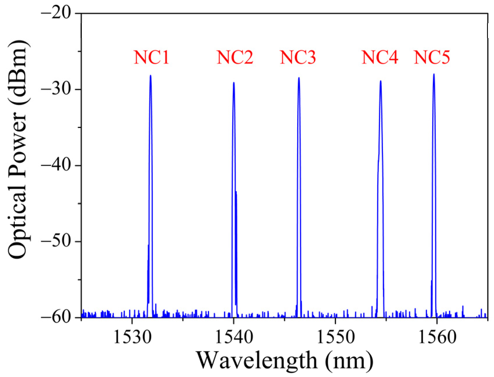
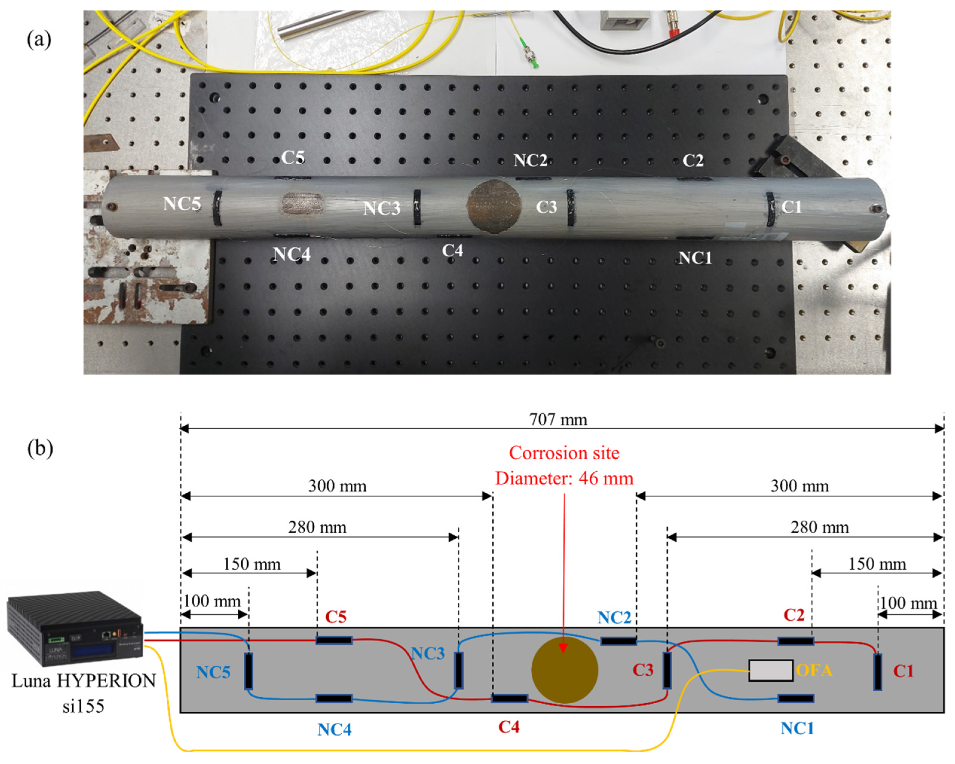
- two identical FBG arrays inscribed in single-mode GF1AA optical fiber samples (Thorlabs, Newton, NJ, USA), each containing five gratings, which were later fixed to the pipeline section. One array was fixed to the coating (sensors C1 (1532 nm), C2 (1540 nm), C3 (1547 nm), C4 (1554 nm), and C5 (1559 nm)), and the other was fixed to the steel or non-coating areas (sensors NC1 (1532 nm), NC2 (1540 nm), NC3 (1547 nm), NC4 (1554 nm), and NC5 (1559 nm), as Figure 1 shows);
- ii.
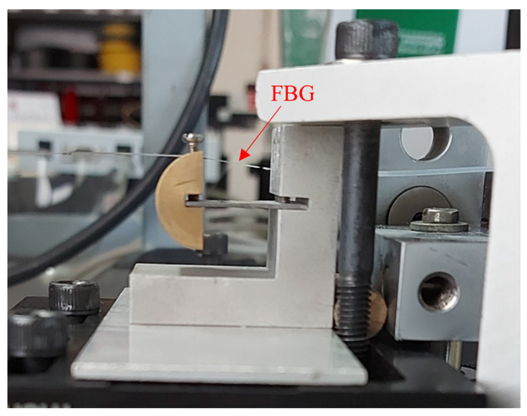
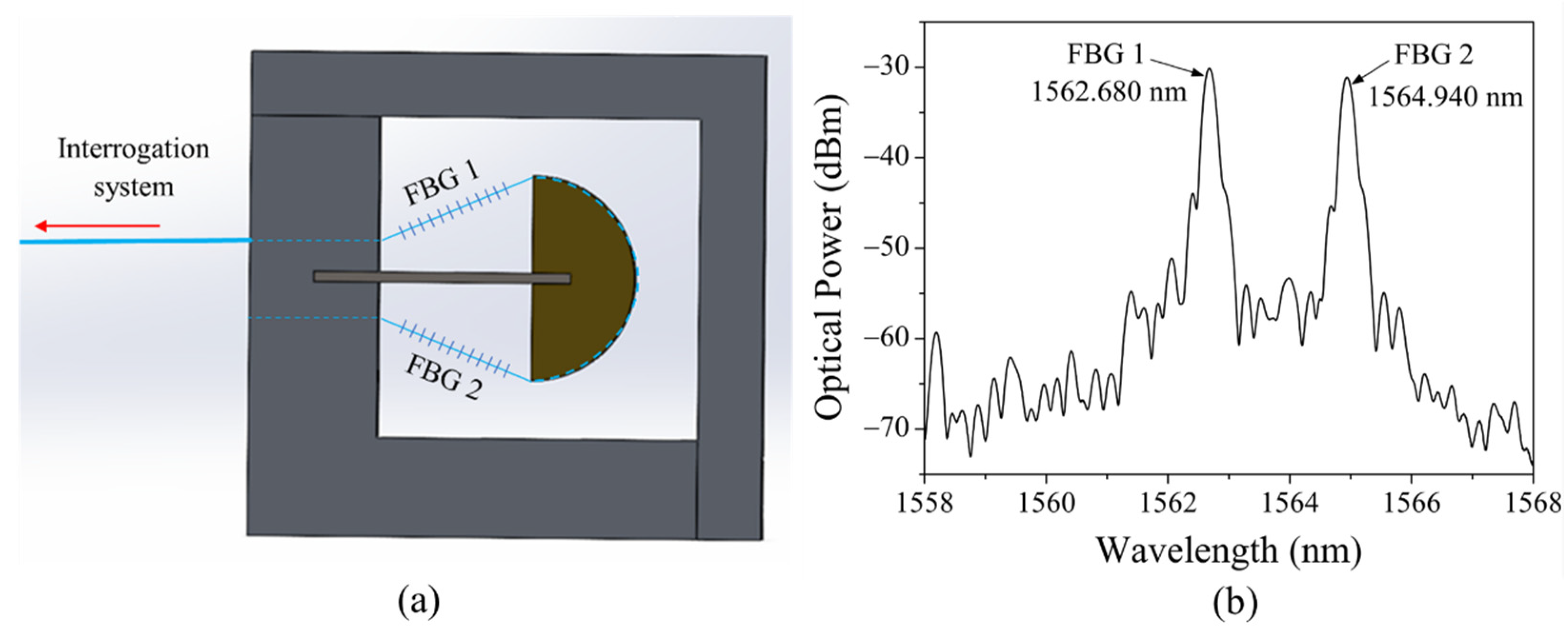
- two FBGs in two different fiber samples and an array with two gratings were inscribed in a single-mode UHNA1 optical fiber (Thorlabs, Newton, NJ, USA) for the OFA. This optical fiber offers low bend losses [56], an important feature for the proposed accelerometer. The two FBGs in different fiber samples were used on different occasions for an initial characterization of the OFA. The array with two FBGs, inscribed in a hydrogenated UHNA1 optical fiber (at a hydrogen pressure of 120 bar for 2 weeks) to enhance the photosensitivity, was used in the final version of the OFA.
2.2. Design and Production of the Optical Fiber Accelerometer
2.2.1. Design
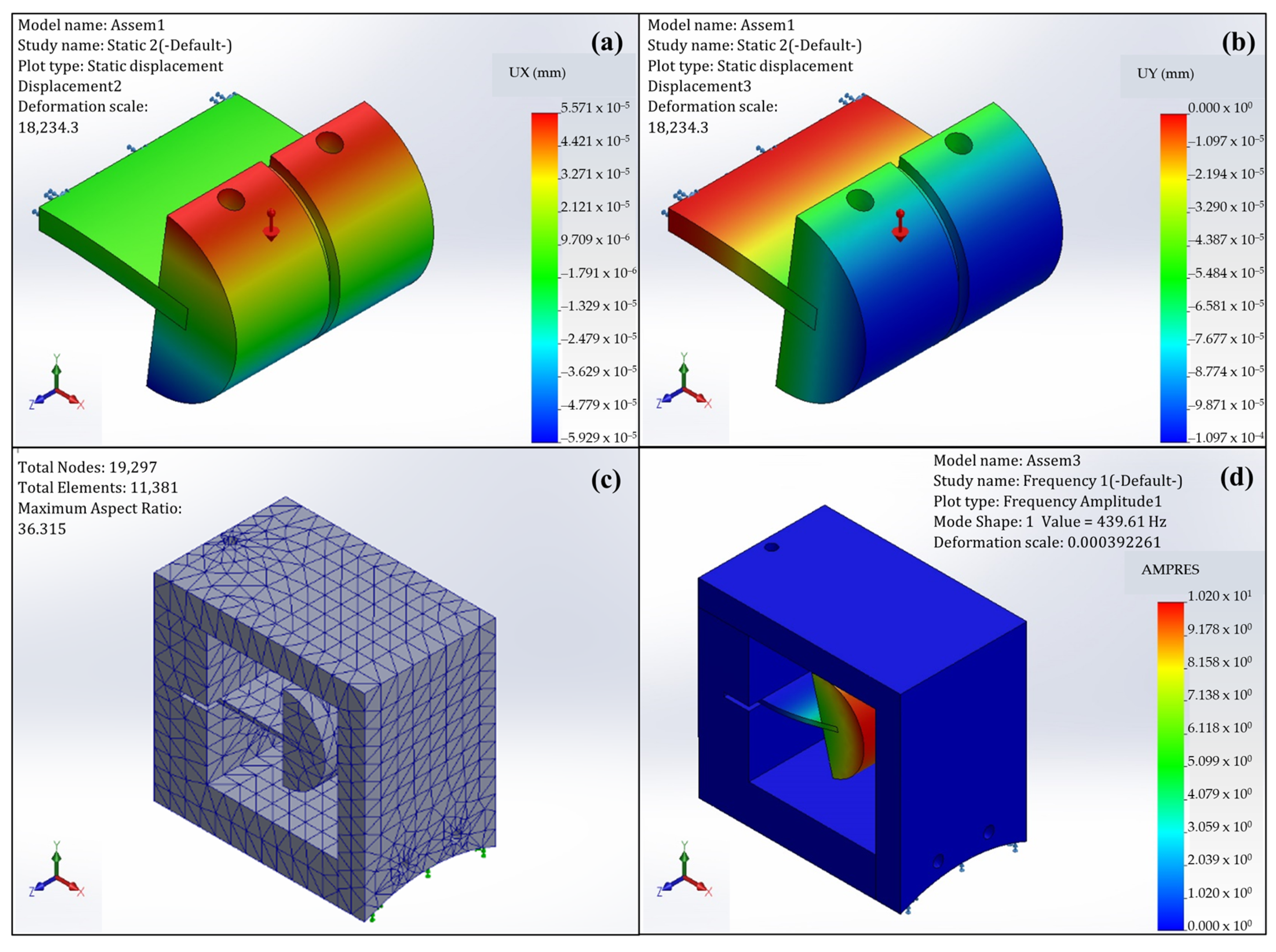
2.2.2. Simulations
2.2.3. Production and Initial Characterization
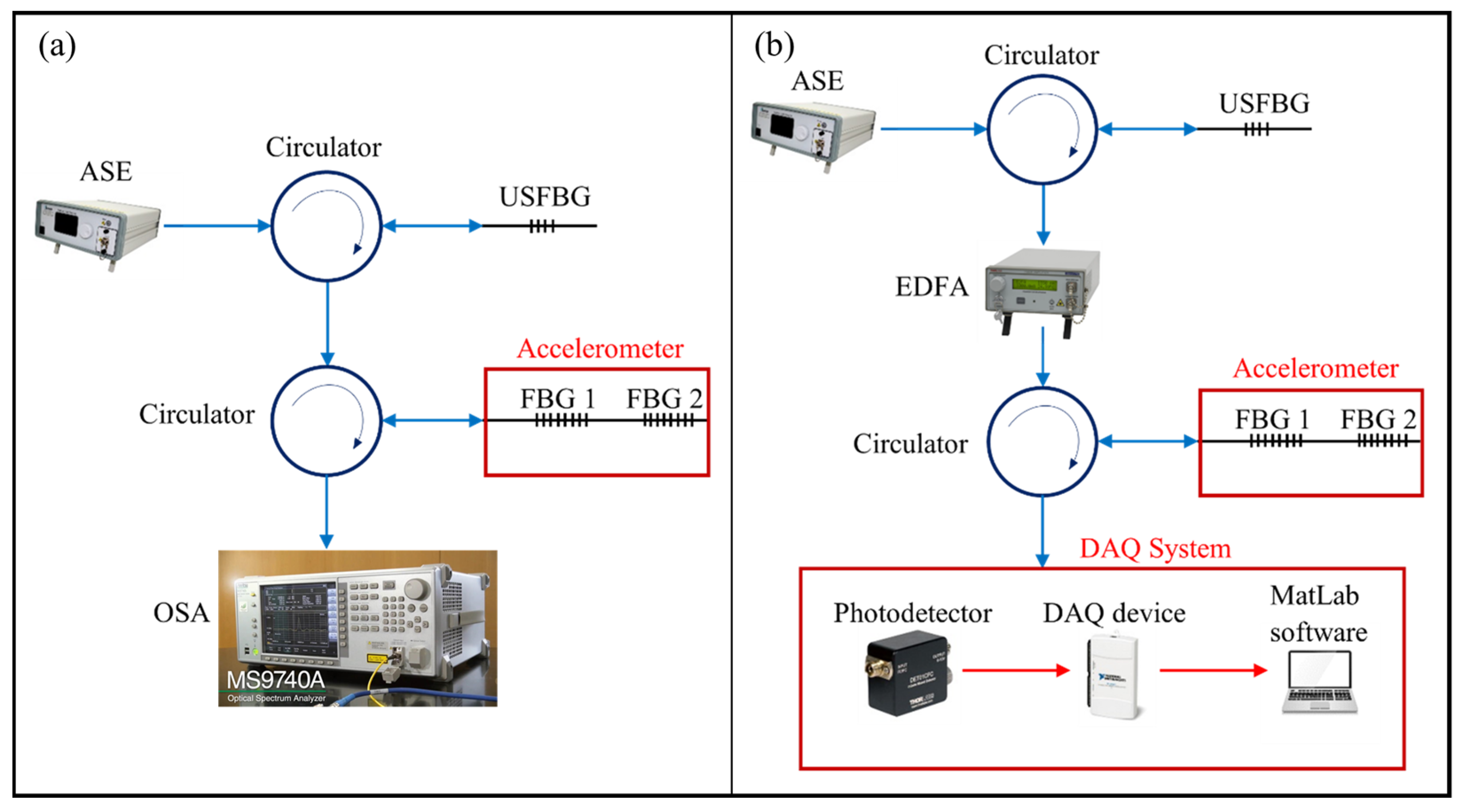
2.2.4. Interrogation Systems
2.3. Natural Frequency Monitoring
2.3.1. Principle of Operation
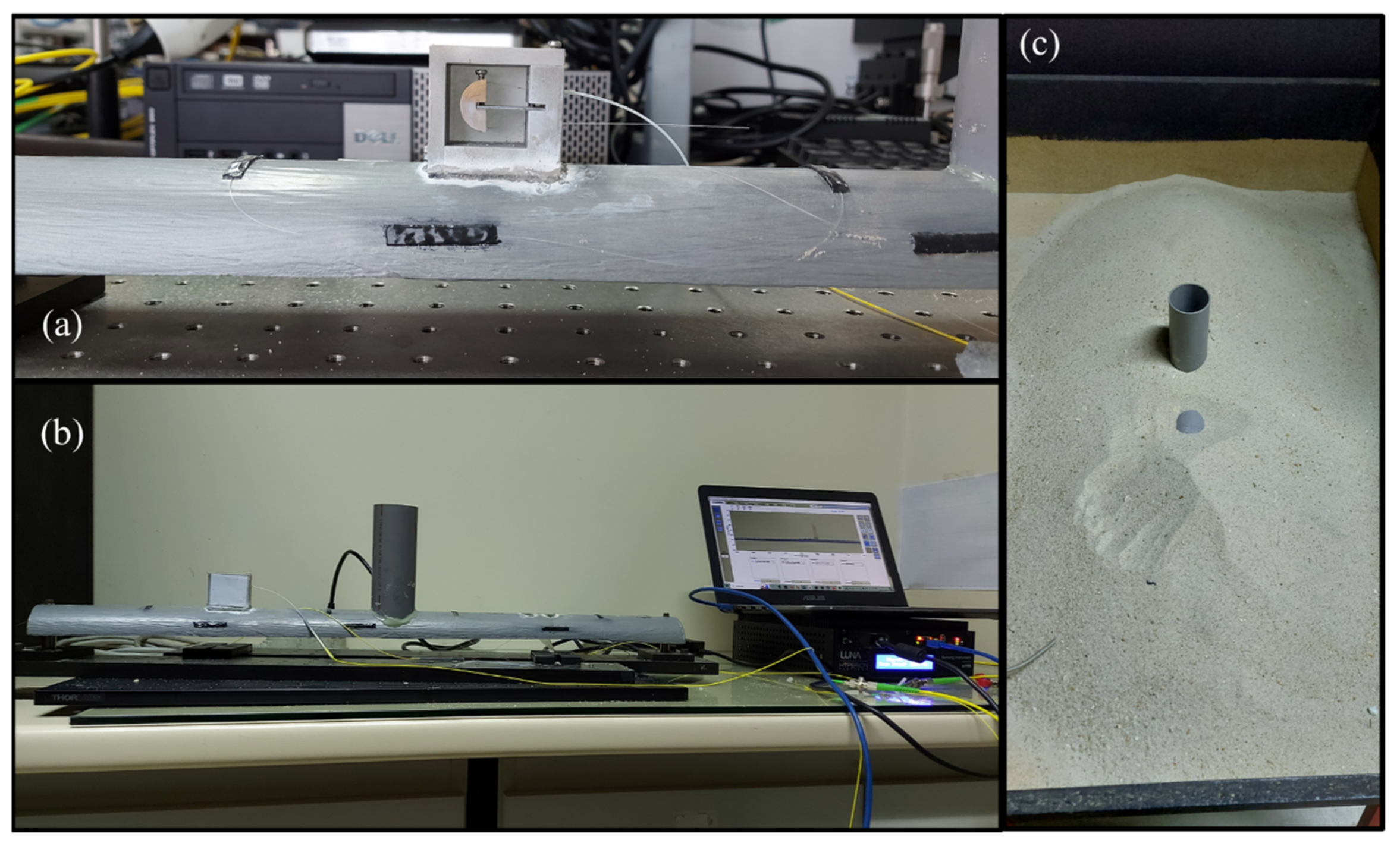
2.3.2. Experimental Procedure
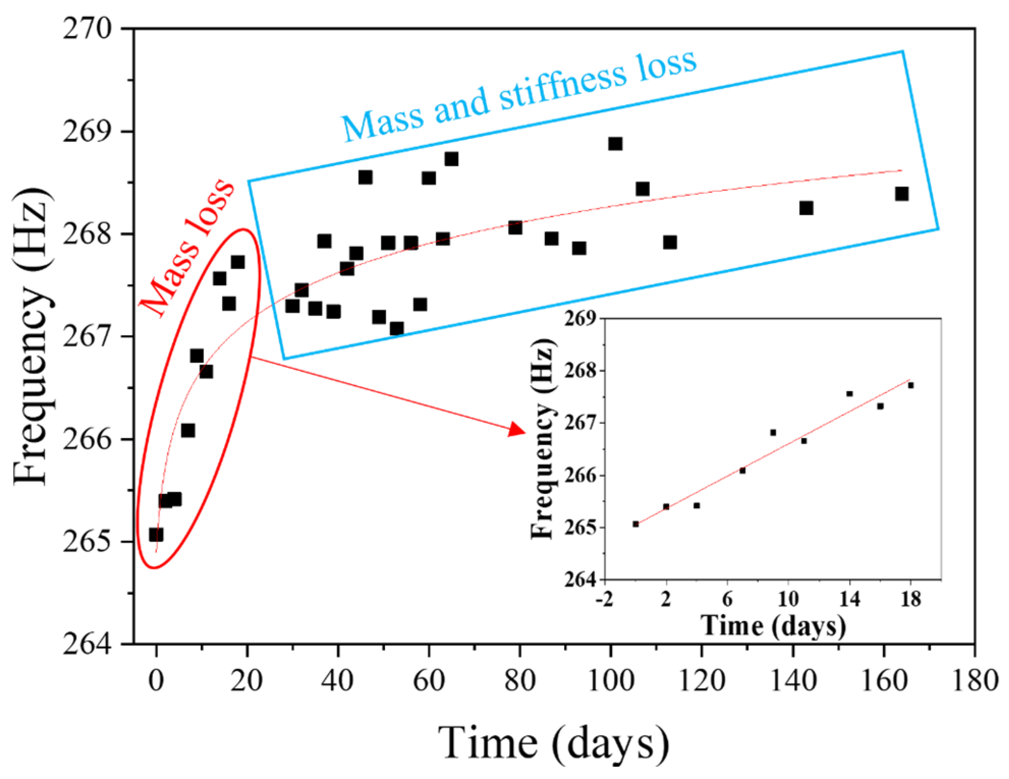
3. Results and Discussion
4. Conclusions
Author Contributions
Funding
Data Availability Statement
Conflicts of Interest
References
- Koch, G. Cost of corrosion. In Trends in Oil and Gas Corrosion Research and Technologies: Production and Transmission, 1st ed.; El-Sherik, A.M., Ed.; Woodhead Publishing: Sawston, UK, 2017; pp. 3–30. [Google Scholar]
- Gentil, V. Corrosão, 3rd ed.; Livros Técnicos e Científicos Editora S.A.: Rio de Janeiro, Brazil, 1996. [Google Scholar]
- Sahu, S.; Frankel, G.S. Effect of substrate orientation and anisotropic strength on corrosion pits. Corros. Sci. 2023, 211, 110772. [Google Scholar] [CrossRef]
- Senior, N.A.; Martino, T.; Diomidis, N.; Gaggiano, R.; Binns, J.; Keech, P. The measurement of ultra low uniform corrosion rates. Corros. Sci. 2020, 176, 108913. [Google Scholar] [CrossRef]
- Lee, Y.-H.; Byun, J.-H.; Ko, S.-J.; Park, E.-H.; Kim, J.-G. Effect of oxygen on pitting corrosion of copper pipe in fire sprinkler system. Mater. Chem. Phys. 2023, 301, 127584. [Google Scholar] [CrossRef]
- Zhang, X.; Zhao, S.; Wang, Z.; Li, J.; Qiao, L. The pitting to uniform corrosion evolution process promoted by large inclusions in mooring chain steels. Mater. Charact. 2021, 181, 111456. [Google Scholar] [CrossRef]
- Teixeira, A.P.; Guedes Soares, C.; Netto, T.A.; Estefen, S.F. Reliability of pipelines with corrosion defects. Int. J. Press. Vessels Pip. 2008, 85, 228–237. [Google Scholar] [CrossRef]
- Lu, H.; Xi, D.; Qin, G. Environmental risk of oil pipeline accidents. Sci. Total Environ. 2023, 874, 162386. [Google Scholar] [CrossRef] [PubMed]
- Ramírez-Camacho, J.G.; Carbone, F.; Pastor, E.; Bubbico, R.; Casal, J. Assessing the consequences of pipeline accidents to support land-use planning. Saf. Sci. 2017, 97, 34–42. [Google Scholar] [CrossRef]
- Bubbico, R. A statistical analysis of causes and consequences of the release of hazardous materials from pipelines. The influence of layout. J. Loss Prev. Process Ind. 2018, 56, 458–466. [Google Scholar] [CrossRef]
- Zou, F.; Cegla, F.B. On quantitative corrosion rate monitoring with ultrasound. J. Electroanal. Chem. 2018, 812, 115–121. [Google Scholar] [CrossRef]
- Sun, X.; Zhang, M.; Gao, W.; Guo, C.; Kong, Q. A novel method for steel bar all-stage pitting corrosion monitoring using the feature-level fusion of ultrasonic direct waves and coda waves. Struct. Health Monit. 2023, 22, 714–729. [Google Scholar] [CrossRef]
- Thibbotuwa, U.C.; Cortés, A.; Irizar, A. Ultrasound-Based Smart Corrosion Monitoring System for Offshore Wind Turbines. Appl. Sci. 2022, 12, 808. [Google Scholar] [CrossRef]
- Yaacoubi, S.; El Mountassir, M.; Ferrari, M.; Dahmene, F. Measurement investigations in tubular structures health monitoring via ultrasonic guided waves: A case of study. Measurement 2019, 147, 106800. [Google Scholar] [CrossRef]
- El Mountassir, M.; Yaacoubi, S.; Dellagi, S.; Sfar, M.; Aouini, M. An ultrasonic guided waves based prognostic approach for predictive maintenance: Experimental study cases. Mech. Syst. Signal Process. 2023, 190, 110135. [Google Scholar] [CrossRef]
- Ahmad, R.; Banerjee, S.; Kundu, T. Pipe wall damage detection in buried pipes using guided waves. J. Press. Vessel Technol. Trans. ASME 2009, 131, 011501. [Google Scholar] [CrossRef]
- Gao, L.; Song, H.; Liu, H.; Han, C.; Chen, Y. Model Test Study on Oil Leakage and Underground Pipelines Using Ground Penetrating Radar. Russ. J. Nondestruct. Test. 2020, 56, 435–444. [Google Scholar] [CrossRef]
- Shokri, N.H.; Amin, Z.M.; Seli, V.A. Non-Destruction Method for Detecting Corroded Underground Pipe Using Ground Penetrating Radar. IOP Conf. Ser. Earth Environ. Sci. 2020, 540, 012027. [Google Scholar] [CrossRef]
- Liu, H.; Zhong, J.; Ding, F.; Meng, X.; Liu, C.; Cui, J. Detection of early-stage rebar corrosion using a polarimetric ground penetrating radar system. Constr. Build. Mater. 2022, 317, 125768. [Google Scholar] [CrossRef]
- Wang, X.; Chen, Z.; Guo, E.; Kang, H.; Cao, Z.; Fu, Y.; Wang, T. Corrosion process of Mg–Sn alloys revealed via in situ synchrotron X-ray radiography. Mater. Lett. 2022, 308, 131139. [Google Scholar] [CrossRef]
- Ewert, U.; Tschaikner, M.; Hohendorf, S.; Bellon, C.; Haith, M.I.; Huthwaite, P.; Lowe, M.J.S. Corrosion monitoring with tangential radiography and limited view computed tomography. AIP Conf. Proc. 2016, 1706, 110003. [Google Scholar]
- Wu, R.; Zhang, H.; Yang, R.; Chen, W.; Chen, G. Nondestructive Testing for Corrosion Evaluation of Metal under Coating. J. Sens. 2021, 2021, 6640406. [Google Scholar] [CrossRef]
- Edalati, K.Ã.; Rastkhah, N.; Kermani, A.; Seiedi, M.; Movafeghi, A. The use of radiography for thickness measurement and corrosion monitoring in pipes. Int. J. Press. Vessels Pip. 2006, 83, 736–741. [Google Scholar] [CrossRef]
- He, Y.; Tian, G.; Zhang, H.; Alamin, M.; Simm, A.; Jackson, P. Steel corrosion characterization using pulsed eddy current systems. IEEE Sens. J. 2012, 12, 2113–2120. [Google Scholar] [CrossRef]
- Butusova, Y.N.; Mishakin, V.V.; Kachanov, M. On monitoring the incubation stage of stress corrosion cracking in steel by the eddy current method. Int. J. Eng. Sci. 2020, 148, 103212. [Google Scholar] [CrossRef]
- Mardaninejad, R.; Safizadeh, M.S. Gas Pipeline Corrosion Mapping Through Coating Using Pulsed Eddy Current Technique. Russ. J. Nondestruct. Test. 2019, 55, 858–867. [Google Scholar] [CrossRef]
- Doshvarpassand, S.; Wu, C.; Wang, X. An overview of corrosion defect characterization using active infrared thermography. Infrared Phys. Technol. 2019, 96, 366–389. [Google Scholar] [CrossRef]
- Elizalde, J.S.G.; Chiou, Y.S. Improving the detectability and confirmation of hidden surface corrosion on metal sheets using active infrared thermography. J. Build. Eng. 2023, 66, 105931. [Google Scholar] [CrossRef]
- Yu, S.; Chung, W.W.; Lau, T.C.; Lai, W.W.; Sham, J.F.C.; Ho, C.Y. Laboratory validation of in-pipe pulsed thermography in the rapid assessment of external pipe wall thinning in buried metallic utilities. NDT E Int. 2023, 135, 102791. [Google Scholar] [CrossRef]
- Hren, M.; Kosec, T.; Legat, A. Characterization of Stainless Steal Corrosion Processes in Mortar Using Various Monitoring Techniques. Constr. Build. Mater. 2019, 221, 604–613. [Google Scholar] [CrossRef]
- Pereira, E.V.; Figueira, R.B.; Salta, M.M.L.; Fonseca, I.T.E. A Galvanic Sensor for Monitoring the Corrosion Condition of the Concrete Reinforcing Steel: Relationship Between the Galvanic and the Corrosion Currents. Sensors 2009, 9, 8391–8398. [Google Scholar] [CrossRef]
- Tu, G.; Zhang, X.; Zhang, Y.; Ying, Z.; Lv, L. Strain variation measurement with short-time Fourier transform-based Brillouin optical time-domain reflectometry sensing system. Electron. Lett. 2014, 50, 1624–1626. [Google Scholar] [CrossRef]
- Ma, W.; Jiang, Y.; Zhang, H.; Zhang, L.; Hu, J.; Jiang, L. Miniature on-fiber extrinsic Fabry-Perot interferometric vibration sensors based on micro-cantilever beam. Nanotechnol. Rev. 2019, 8, 293–298. [Google Scholar] [CrossRef]
- Jin, X.; Sun, C.; Duan, S.; Liu, W.; Li, G.; Zhang, S.; Chen, X.; Zhao, L.; Lu, C.; Yang, X.; et al. High strain sensitivity temperature sensor based on a secondary modulated tapered long period fiber grating. IEEE Photonics J. 2019, 11, 7100908. [Google Scholar] [CrossRef]
- Ye, X.W.; Ni, Y.Q.; Yin, J.H. Safety Monitoring of Railway Tunnel Construction Using FBG Sensing Technology. Adv. Struct. Eng. 2013, 16, 1401–1409. [Google Scholar] [CrossRef]
- Rao, Y.-J. In-fibre Bragg grating sensors. Meas. Sci. Technol. 1997, 8, 355–375. [Google Scholar] [CrossRef]
- Hong, C.; Yuan, Y.; Yang, Y.; Zhang, Y.; Abro, Z.A. A simple FBG pressure sensor fabricated using fused deposition modelling process. Sens. Actuators A Phys. 2019, 285, 269–274. [Google Scholar] [CrossRef]
- Liu, Z.; Gu, X.; Wu, C.; Ren, H.; Zhou, Z.; Tang, S. Studies on the validity of strain sensors for pavement monitoring: A case study for a fiber Bragg grating sensor and resistive sensor. Constr. Build. Mater. 2022, 321, 126085. [Google Scholar] [CrossRef]
- Zhao, X.; Jia, Z.; Fan, W.; Liu, W.; Gao, H.; Yang, K.; Yu, D. A Fiber Bragg Grating acceleration sensor with temperature compensation. Optik 2021, 241, 166993. [Google Scholar] [CrossRef]
- Kokhanovskiy, A.; Shabalov, N.; Dostovalov, A.; Wolf, A. Highly dense FBG temperature sensor assisted with deep learning algorithms. Sensors 2021, 21, 6188. [Google Scholar] [CrossRef]
- Yan, G.; Wang, T.; Zhu, L.; Meng, F.; Zhuang, W. A novel strain-decoupled sensitized FBG temperature sensor and its applications to aircraft thermal management. Opt. Laser Technol. 2021, 140, 106597. [Google Scholar] [CrossRef]
- Wang, D.; Wu, Y.; Song, Y.; Wang, Y.; Zhu, L. A double-mass block acceleration sensor based on FBG. Opt. Fiber Technol. 2021, 66, 102681. [Google Scholar] [CrossRef]
- Sun, M.; Shi, B.; Zhang, D.; Feng, C.; Wu, J.; Wei, G. Pipeline leakage monitoring experiments based on evaporation-enhanced FBG temperature sensing technology. Struct. Control Health Monit. 2021, 28, e2691. [Google Scholar] [CrossRef]
- Ren, L.; Jia, Z.; Li, H.; Song, G. Design and experimental study on FBG hoop-strain sensor in pipeline monitoring. Opt. Fiber Technol. 2014, 20, 15–23. [Google Scholar] [CrossRef]
- Ren, L.; Jiang, T.; Jia, Z.; Li, D.; Yuan, C.; Li, H. Pipeline corrosion and leakage monitoring based on the distributed optical fiber sensing technology. Measurement 2018, 122, 57–65. [Google Scholar] [CrossRef]
- Wang, J.; Ren, L.; Jia, Z.; Jiang, T.; Wang, G. Pipeline leak detection and corrosion monitoring based on a novel FBG pipe-fixture sensor. Struct. Health Monit. 2022, 21, 1819–1832. [Google Scholar] [CrossRef]
- Shen, N.; Chen, L.; Chen, R. Multi-route fusion method of GNSS and accelerometer for structural health monitoring. J. Ind. Inf. Integr. 2023, 32, 100442. [Google Scholar] [CrossRef]
- Chilamkuri, K.; Kone, V. Monitoring of varadhi road bridge using accelerometer sensor. Mater. Today Proc. 2020, 33, 367–371. [Google Scholar] [CrossRef]
- Pieraccini, M.; Fratini, M.; Parrini, F.; Atzeni, C.; Bartoli, G. Interferometric radar vs. accelerometer for dynamic monitoring of large structures: An experimental comparison. NDT E Int. 2008, 41, 258–264. [Google Scholar] [CrossRef]
- Zhang, H.; Wei, X.; Ding, Y.; Jiang, Z.; Ren, J. A low noise capacitive MEMS accelerometer with anti-spring structure. Sens. Actuators A Phys. 2019, 296, 79–86. [Google Scholar] [CrossRef]
- Lim, K.-S.; Zaini, M.K.A.; Ong, Z.-C.; Abas, F.Z.M.; Salim, M.A.B.M.; Ahmad, H. Vibration Mode Analysis for a Suspension Bridge by Using Low-Frequency Cantilever-Based FBG Accelerometer Array. IEEE Trans. Instrum. Meas. 2021, 70, 7000908. [Google Scholar] [CrossRef]
- Jiang, S.; Wang, Y.; Zhang, F.; Sun, Z.; Wang, C. A high-sensitivity FBG accelerometer and application for flow monitoring in oil wells. Opt. Fiber Technol. 2022, 74, 103128. [Google Scholar] [CrossRef]
- Le, H.-D.; Chiang, C.-C.; Nguyen, C.-N.; Hsu, H.-C. A novel short fiber Bragg grating accelerometer based on a V-type dual mass block structure for low- and medium-frequency vibration measurements. Opt. Laser Technol. 2023, 161, 109131. [Google Scholar] [CrossRef]
- Kim, J.T.; Seong, S.H.; Lee, C.K.; Hur, S.; Lee, N.Y.; Lee, S.J. Flow-accelerated corrosion monitoring through advanced sensors. Adv. Sens. Syst. Appl. II 2005, 5634, 404–415. [Google Scholar]
- Kashyap, R. Fiber Bragg Gratings, 2nd ed.; Academic Press: San Diego, CA, USA, 2009. [Google Scholar]
- Ultra-High NA Waveguide Splice Fiber. Available online: https://www.thorlabs.com/newgrouppage9.cfm?objectgroup_id=340 (accessed on 26 April 2023).
- Pereira, L.; Min, R.; Woyessa, G.; Bang, O.; Marques, C.; Varum, H.; Antunes, P. Interrogation Method with Temperature Compensation Using Ultra-Short Fiber Bragg Gratings in Silica and Polymer Optical Fibers as Edge Filters. Sensors 2023, 23, 23. [Google Scholar] [CrossRef] [PubMed]
- Pereira, L.; Marques, C.; Min, R.; Woyessa, G.; Bang, O.; Varum, H.; Antunes, P. Bragg Gratings in ZEONEX Microstructured Polymer Optical Fiber With 266-nm Nd:YAG Laser. IEEE Sens. J. 2023, 23, 9308–9316. [Google Scholar] [CrossRef]
- Antunes, P.; Varum, H.; André, P. Uniaxial fiber Bragg grating accelerometer system with temperature and cross axis insensitivity. Measurement 2011, 44, 55–59. [Google Scholar] [CrossRef]
- Díaz, C.A.R.; Leitão, C.; Marques, C.A.; Domingues, M.F.; Alberto, N.; Pontes, M.J.; Frizera, A.; Ribeiro, M.R.N.; André, P.S.B.; Antunes, P.F.C. Low-cost interrogation technique for dynamic measurements with FBG-based devices. Sensors 2017, 17, 2414. [Google Scholar] [CrossRef] [PubMed]
- Demeter, G.F. Dynamics and Vibration of Structures; Wiley: New York, NY, USA, 1973; pp. 31–35. [Google Scholar]
- Razak, H.A.; Choi, F.C. The effect of corrosion on the natural frequency and modal damping of reinforced concrete beams. Eng. Struct. 2001, 23, 1126–1133. [Google Scholar] [CrossRef]
- Sousa, I.; Pereira, L.; Mesquita, E.; Souza, V.L.; Araújo, W.S.; Cabral, A.; Alberto, N.; Varum, H.; Antunes, P. Sensing System Based on FBG for Corrosion Monitoring in Metallic Structures. Sensors 2022, 22, 5947. [Google Scholar] [CrossRef]
- Yang, C.; Liang, K.; Zhang, X.; Geng, X. Sensor placement algorithm for structural health monitoring with redundancy elimination model based on sub-clustering strategy. Mech. Syst. Signal Process. 2019, 124, 369–387. [Google Scholar] [CrossRef]
- Yang, C.; Xia, Y. Interval Pareto front-based multi-objective robust optimization for sensor placement in structural modal identification. Reliab. Eng. Syst. Saf. 2024, 242, 109703. [Google Scholar] [CrossRef]


| Cantilever Dimensions (mm) | Simulated Results | Experimental Results | ||||
|---|---|---|---|---|---|---|
| Length | Width | Thickness | SA (pm/g) | fn_OFA (Hz) | SA (pm/g) | fn_OFA (Hz) |
| 20 | 20 | 2.0 | 4.3 | 1566.5 | 5.5 | 1047.0 |
| 20 | 20 | 1.5 | 10.3 | 1030.5 | - | - |
| 20 | 20 | 1.0 | 34.1 | 608.2 | - | - |
| 20 | 20 | 0.8 | 65.9 | 439.6 | 66.5 | 374.4 |
| fn_pipeline (Hz) | |||||||||||
|---|---|---|---|---|---|---|---|---|---|---|---|
| Situation | C1 | C2 | C3 | C4 | C5 | NC1 | NC2 | NC3 | NC4 | NC5 | OFA |
| 1 | 140.3 | 140.3 | 140.3 | 140.3 | 140.3 | 140.5 | 140.6 | 140.5 | 140.6 | 140.6 | 140.8 |
| 288.7 | 288.4 | 288.2 | 288.4 | 288.1 | 288.4 | 288.4 | 288.4 | 288.4 | 288.4 | 288.2 | |
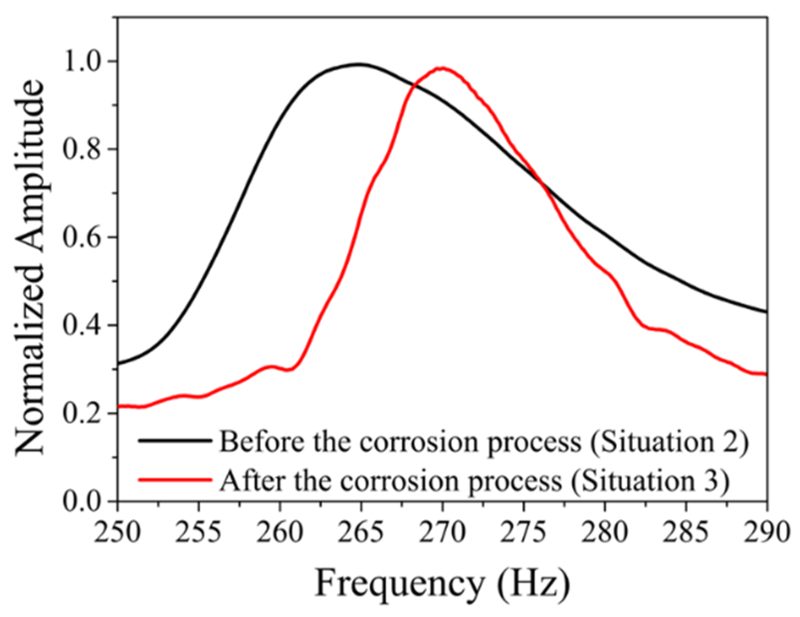
| 2 | - | - | - | - | - | - | - | - | - | - | 265.1 |
| 3 | 135.7 | 135.7 | 135.7 | 135.7 | 135.7 | 135.7 | 135.7 | 135.9 | 135.7 | 135.9 | 135.7 |
| - | - | - | - | - | - | - | - | - | - | 269.8 | |
Disclaimer/Publisher’s Note: The statements, opinions and data contained in all publications are solely those of the individual author(s) and contributor(s) and not of MDPI and/or the editor(s). MDPI and/or the editor(s) disclaim responsibility for any injury to people or property resulting from any ideas, methods, instructions or products referred to in the content. |
© 2024 by the authors. Licensee MDPI, Basel, Switzerland. This article is an open access article distributed under the terms and conditions of the Creative Commons Attribution (CC BY) license (https://creativecommons.org/licenses/by/4.0/).
Share and Cite
Pereira, L.; Sousa, I.; Mesquita, E.; Cabral, A.; Alberto, N.; Diaz, C.; Varum, H.; Antunes, P. FBG-Based Accelerometer for Buried Pipeline Natural Frequency Monitoring and Corrosion Detection. Buildings 2024, 14, 456. https://doi.org/10.3390/buildings14020456
Pereira L, Sousa I, Mesquita E, Cabral A, Alberto N, Diaz C, Varum H, Antunes P. FBG-Based Accelerometer for Buried Pipeline Natural Frequency Monitoring and Corrosion Detection. Buildings. 2024; 14(2):456. https://doi.org/10.3390/buildings14020456
Chicago/Turabian StylePereira, Luís, Israel Sousa, Esequiel Mesquita, Antônio Cabral, Nélia Alberto, Camilo Diaz, Humberto Varum, and Paulo Antunes. 2024. "FBG-Based Accelerometer for Buried Pipeline Natural Frequency Monitoring and Corrosion Detection" Buildings 14, no. 2: 456. https://doi.org/10.3390/buildings14020456
APA StylePereira, L., Sousa, I., Mesquita, E., Cabral, A., Alberto, N., Diaz, C., Varum, H., & Antunes, P. (2024). FBG-Based Accelerometer for Buried Pipeline Natural Frequency Monitoring and Corrosion Detection. Buildings, 14(2), 456. https://doi.org/10.3390/buildings14020456