Data-Driven Decision Support for Equipment Selection and Maintenance Issues for Buildings

Abstract

Equipment costs play a critical role in decision making during design and construction, which requires up-to-date information and data. The design of this study incorporates the inputs from the literature review on the influencing factors of equipment costs and major targeted equipment types to enhance decision support for equipment selection, project construction, and maintenance issues. Two traditional cost estimation methods and five machine-learning methods were compared in this study to identify significant attributes related to the predictions of the costs and residual values of each targeted equipment type. The novelty of this study is that the developed method improves prediction accuracy by establishing a comprehensive and well-structured database framework. A comparison of this method with the existing prediction models reveals that the results and the accuracy of multiple regression analysis are improved in the range of (3% to 33.97%) with the use of a modified decision-tree model combined with support vector machines. The major contribution of this research is the design, implementation, and validation of a machine-learning-based modified decision tree with a support vector machine model for improved accuracy and decision support in construction management. Future research should consider the relationship between geographical variations and value changes.

1. Introduction

Equipment costs are essential for decision making in a project lifecycle, especially for bidding, cost control, maintenance, and reimbursement purposes. One reason is that equipment costs can considerably affect project profitability. Consequently, industry professionals need to spend an enormous amount of time searching for an alternative when the original quoted piece of equipment is unavailable. The calculation should consider ownership, operating, and miscellaneous costs like mobilization and inspection. The corresponding accuracy relies on the quality of cost data sources, which, however, becomes a serious issue [1]. Specifically, contractors who work on a small number of projects are usually reluctant to purchase data sources [2]. Secondly, only limited transparency and debatable local adjustments are available in some data sources. Subscribers have little knowledge of how the information is gathered, its cost categories, and how the rates are determined [3,4]. Thirdly, it is difficult to correlate adjusted costs from a data source to factual data, which defeats the purpose of data-driven decision making and fair competition. Lastly, equipment data becomes obsolete in some data sources (e.g., [5]). Hence, the engineering and construction industries are in urgent need of a user-friendly and intelligent equipment value prediction framework, which can monitor the changes in the major factors influencing the costs, update the corresponding rates, and inform industry practitioners and stakeholders when major changes happen.

This research aims to develop an accurate and publicly accessible model framework with the capacity for trend-pattern identification and the suggestions of a supporting database for equipment cost prediction. As an essential part of equipment cost, residual value is the remaining value of an asset at the end of its useful life. It is affected by the time value of money (TVM), which is crucial in the context of an economic crisis, such as high inflation [6]. Improving the quality and reliability of data sources can help make accurate cost estimates. The next section in this paper is the literature review, which first compares the traditional estimating methods and models, and machine-learning algorithms. The components of the model inputs are from the literature review as well and are described in the research design (see the Section 3). They are integrated as the influencing factors of the equipment cost estimates and major targeted equipment types. The collected data are from public databases to provide data attributes for the cost and residual value prediction of the targeted equipment types. Based on the factors, the appropriate costs are identified, and a durable and reliable model is developed by incorporating various machine-learning techniques.

The novelty of this model is the improved prediction accuracy from utilizing the latest, comprehensive, well-structured datasets to train the model. Furthermore, this automated and intelligent method integrates the advantages of the decision tree, random forest, and support vector machine (SVM) algorithms to lower computation time, reduce the possibility of overfitting by using multiple trees, and enhance prediction accuracy.

2. Literature Review

2.1. Estimating Methods and Models

Predicting equipment costs involves utilizing various tools and algorithms, and usually relies on the availability of contexts and data.

Table 1. Typical tools and algorithms for equipment cost prediction.

Tools	Description	Advantages	Disadvantages
Cost Indexes	The indexes track changes in costs over time based on industry-specific factors and adjust historical cost data to current values.	(1) Adaptability based on industry-specific factors. (2) Widely accepted.	(1) Generalization: some project-specific factors are not considered. (2) Time lag leading to inaccuracies.
Expert Judgment (i.e., Delphi Method)	Expert opinions and judgment are valuable, especially when dealing with unique or specialized equipment. A Delphi method starts with obtaining input from a panel of experts through a structured and iterative process to reach a consensus on equipment costs.	(1) Expert insight. (2) Flexibility: applicable when data is limited or for unique projects.	(1) Subjectivity. (2) Resource intensive: the Delphi method has multiple rounds of expert input and is time-consuming.
Historical Data Analysis	This is considered analogous estimating, which uses historical data from similar scenarios to estimate equipment costs for a new scenario. It relies on the assumption that similar scenarios have similar cost structures.	(1) Practical with real-world data. (2) Context sensitivity: considers the specific characteristics of similar projects.	(1) Limited applicability for unique projects with significant differences. (2) Data quality relies on the availability and quality of historical data.
Monte Carlo Simulation	By simulating a large number of possible outcomes to account for uncertainty and variability in equipment costs, this method can handle high uncertainty.	(1) Risk assessment. (2) Comprehensive: various input distributions and scenarios.	(1) Complex and computationally intensive. (2) Requires accurate data and assumptions about probability distributions.
Cost Estimation Software like 2024 CostWorks Estimator® and Parametric Estimation Tools	These tools use historical data and mathematical relationships (see Figure 1) to estimate costs based on key parameters. Parametric models for equipment cost prediction are industry-specific and customizable for different types of equipment.	(1) Efficiency: rapid cost estimates based on key parameters. (2) Easiness: user-friendly.	(1) Sensitivity to assumptions: accuracy of the assumptions and input parameters. (2) Limited flexibility: no complex relationships between variables.
Regression Analysis	(1) Linear regression: This statistical method models the relationship between independent variables (equipment features) and the dependent variable (cost). (2) Multiple regression: multiple independent variables and allows for complex modeling of cost factors.	(1) Interpretability. (2) Versatility: applicable to various types of data and well-suited to linear relationships.	(1) Assumption of linearity. (2) Limited complexity.
Machine-Learning (ML) Algorithms	Commonly used ML algorithms include: (1) Decision trees for both categorical and numerical data, versatile for different types of input features. (2) Random forest combining multiple decision trees, providing improved accuracy and robustness. (3) Gradient-boosting algorithms for regression tasks and complex relationships. (4) Deep-learning models (e.g., neural networks) for large and complex datasets, intricate patterns, and relationships.	(1) Capturing complex relationships and complex patterns. (2) High accuracy, especially with large and diverse datasets.	(1) Black-box nature: challenging to interpret. (2) Data intensiveness: substantial amounts of data for training. (3) Overfitting: providing accurate predictions for training data but not for newly added data.

lists some commonly used tools and algorithms for predicting equipment costs. For example, to accurately estimate equipment costs, industry professionals rely on using commercial guides or databases as resources for fair prices. Yet, using a commercial cost database is considered advantageous to cost guides as professionals do not need to create or maintain the database. Additionally, such databases have extensive and current equipment information (e.g., updated bi-annually) and are better adjusted for regional and local variables than cost guides. However, such a data acquisition is a burden to contractors because they need to purchase annual subscriptions. For example, the Bluebook database costs approximately 6000 USD/year per subscription [2].

Figure 1 shows the typical cost components in an equipment hourly rate prediction that is still in use today. Yet, there is a lack of understanding of definitive methods to estimate reasonable equipment costs, especially small amounts of work [2,7,8,9]. Comparing the results from using different cost guides, a significant variance exists across all types of equipment, which indicates that each organization estimates costs based on its typical means and methods. The geographical features of data can affect prediction accuracy [2,7,8,9]. People need to spend a significant amount of time to estimate, review, and audit costs if there are no acceptable, reliable, and user-friendly methods. Hence, the creation of an automated and accurate method to update and predict equipment costs is a challenge.

2.2. Multivariate Analysis and Machine Learning

Recently, a few cost-predicting models like classification and regression trees (CART), modified decision trees (MDT), and recursive neural networks (RNNs) were developed to describe multivariate interactions [10,11].

Table 2. Comparison of machine-learning algorithms for cost prediction.

References	Contents	Dataset
[12]	This study used an Advanced Regression Techniques (ART) method and categorical features as factors to predict rental apartment prices. The selected algorithms were (1) advanced linear regression, neural network, random forest, support vector machine (SVM), and decision-tree regressor for predictors; (2) Ensemble AdaBoosting Regressor, Ensemble Gradient Boosting Regressor, and Ensemble eXtreme Gradient Boosting (XGBoost) for ensemble learning; and (3) Ridge Regression, Lasso Regression, and Elastic Net Regression to combine the advance regression techniques.	The dataset was from bProperty.com about the apartments in the city of Dhaka, Bangladesh.
[13]	An encoder–decoder framework and a dual-gated recurrent unit (GRU) were used to calculate a house popularity feature through inter-event time, which was the gap between two successive reviews. The comparison between Long-Short-Term Memory (LSTM) and GRU algorithms showed that GRU algorithms had better time efficiency and less computation complexity. The dual-state gates allowed the gates to ignore irrelevant information. The TensorFlow library was used to develop the model.	The datasets of review comments were from vacation rental websites. The parameters were limited.
[14]	This study summarized the knowledge body on machine-learning algorithms and deep-learning approaches for construction cost prediction. But it only considered building, bridge, tower, dam, road, highway, railroad, airport, and tunnel costs. The selected algorithms of unsupervised learning detected unlabeled instances of data using the clustering learning method, such as Expectation-Maximization (EM) clustering, K-means clustering, and Self Organizing Map (SOM). The selected supervised learning implemented the detection (or classification) depending on the labeled instances of data in a training stage, which includes SVM, decision tree, random forest, naive Bayes (NB), K-nearest neighbors (K-NN), ANN, deep neural network, conventional neural network, and RNN. The evaluation metrics include error, accuracy, and R2. SVM and ANN produced the best outcomes in building and road projects.	Bibliographic records were retrieved from the Scopus database. The findings were incoherent. The research limitations include a lack of a quantitative dataset, impractical tasks, and invalidation.
[15]	This real-estate rent-prediction study used the comparison of seven machine-learning algorithms, including linear regression, multilayer perceptron, random forest, KNN, locally weighted learning, sequential minimal optimization, and KStar algorithms. It focused on three house types—single-family, townhouse, and condo—and considered 21 data attributes (e.g., area space, price, number of beds/bathrooms, rent, school rating, etc.). Then, it used a hierarchical clustering approach based on house type and average rent estimate, and lazy learning algorithms were found to have higher accuracy and lower prediction errors compared to eager learning methods.	Using the Zillow API to collect a dataset of residential housing data for Virginia, US.
[16]	Locality-aware heterogeneous data was converted to linked latent spaces to learn their attributes for a final decision. A data-fusion model was implemented with four modules, including multi-granularity spatial context embedding, item set embedding, text encoder, and numerical feature.	GeoSpatial data from Airbnb.
[17]	A natural language processing approach was implemented based on the semantics of online information from Airbnb, Zillow, schools, public transportation, and crime rate websites for rent prediction. Eager and lazy machine-learning models were implemented, together with a transfer learning model for rent prediction.	Detection of a profitable rental property; online textual resources.
[18]	Due to the inaccuracy of the results of multiple linear regressions, a random forest model and a Generalized Boosted Regression (GBM) packet were used to improve the decision tree. The random forest model generated trees for classification and regression analysis. The GBM models improved the capacity of the decision tree by establishing a loss function in the previous model of gradient descent direction.	Strong model-generalization ability. The prediction accuracy was maintained when situations changed.
[10,19]	A decision-support model was developed based on the comparison results of deep- and machine-learning regression networks. It considered data mining, random forest (RF), decision tree (DT), deep neural network (DNN), and linear regression (LR) based modeling. Four performance metrics (i.e., mean absolute error (MAE), mean squared error (MSE), mean absolute percentage error (MAPE), and coefficient of determination (R2)) were used to measure and compare the developed algorithms’ accuracy. The DT model demonstrated the highest accuracy for the heavy construction equipment-related data that was recorded from public equipment auctions available online. The equipment types were grader, excavator, loader, compactor, asphalt paver, and truck.	The data resources included Mascus USA *, 2018; Machinery Zone, 2019; Machinery Trader, 2020; Iron Planet, 2020; Equipment Trader, 2020; Alibaba, 2020.

* See Table 3 for details.

compares the identified machine-learning approaches that help the implementation and automation of cost models. As [10] suggested, machine-learning algorithms and multivariate regression methods helped to improve the prediction accuracy of the residual value of heavy construction equipment. These methods can also identify the influences of the time value of money.

As shown in Table 2, decision-tree models have been used widely in cost prediction. They start from a statement and then decide on the next step based on whether the statement is true or false. A decision tree can classify (also known as classification tree) or predict numeric values (also known as regression tree). During the calculation process, the values of the root attribute are compared with the attribute quantities of a given dataset. Then, a decision-tree model uses a training dataset to deduce decision rules and predict a class or the value of a target variable. Usually, a decision tree takes a binary shape and the movement direction of the model calculation is decided after the comparison. Since the calculation of equipment cost rates (ECRs) resembles the if–then and true–false decision-making process of a decision-tree algorithm, such an algorithm can develop an accurate ECR model.

Table 1 and Table 2 indicate that the selection of regression models depends on data observations. Moreover, supervised-learning algorithms can be used to solve regression and classification problems of equipment-residual-value predictions. Although the required upfront human intervention of supervised-learning models helps to improve the appropriateness of labeled descriptions on the training dataset, it creates unavoidable limitations. Such disadvantages include vast data preparation and computation time, inefficiency due to unwanted data, consistent demand for updates, and overtrained decision boundaries [20]. In this case, the knowledge gap focused on by this study is how to establish a well-structured database framework to improve the prediction accuracy of equipment costs using machine-learning algorithms. The advantages and disadvantages of supervised-learning methods call for caution in balancing the accuracy, maintenance frequency, and computing time of a prediction algorithm for the ECR model.

2.3. Objectives

The following characteristics are suggested in Table 2 for equipment cost predictions. (1) Comprehensive rates should be included for a multitude of construction equipment categories based on industry standards. (2) Extensibility should be considered for estimating the hourly rates of a piece of equipment if it is not listed in the database. (3) The database should be reasonable and acceptable to public project owners (or agencies) and contractors. (4) The ECR model should have a friendly, intelligent, and web-based user interface that is accessible to various contractors and agencies. (5) The ECRs should allow for standby rates and operation rates, with the adjustments of equipment type, age, region, and other influencing factors identified from the literature review.

A reasonable equipment cost-prediction method can support the establishment of hourly compensation rates for contractor-owned equipment and assist in estimating equipment costs for building projects. Thus, the research objectives of the paper are (1) to identify the machine-learning algorithms, (2) to examine influence factors and data features, and (3) to develop a structured database framework and improve prediction accuracy. To achieve these objectives, the main research question is whether a machine-learning algorithm can enhance the reliability of ECR prediction.

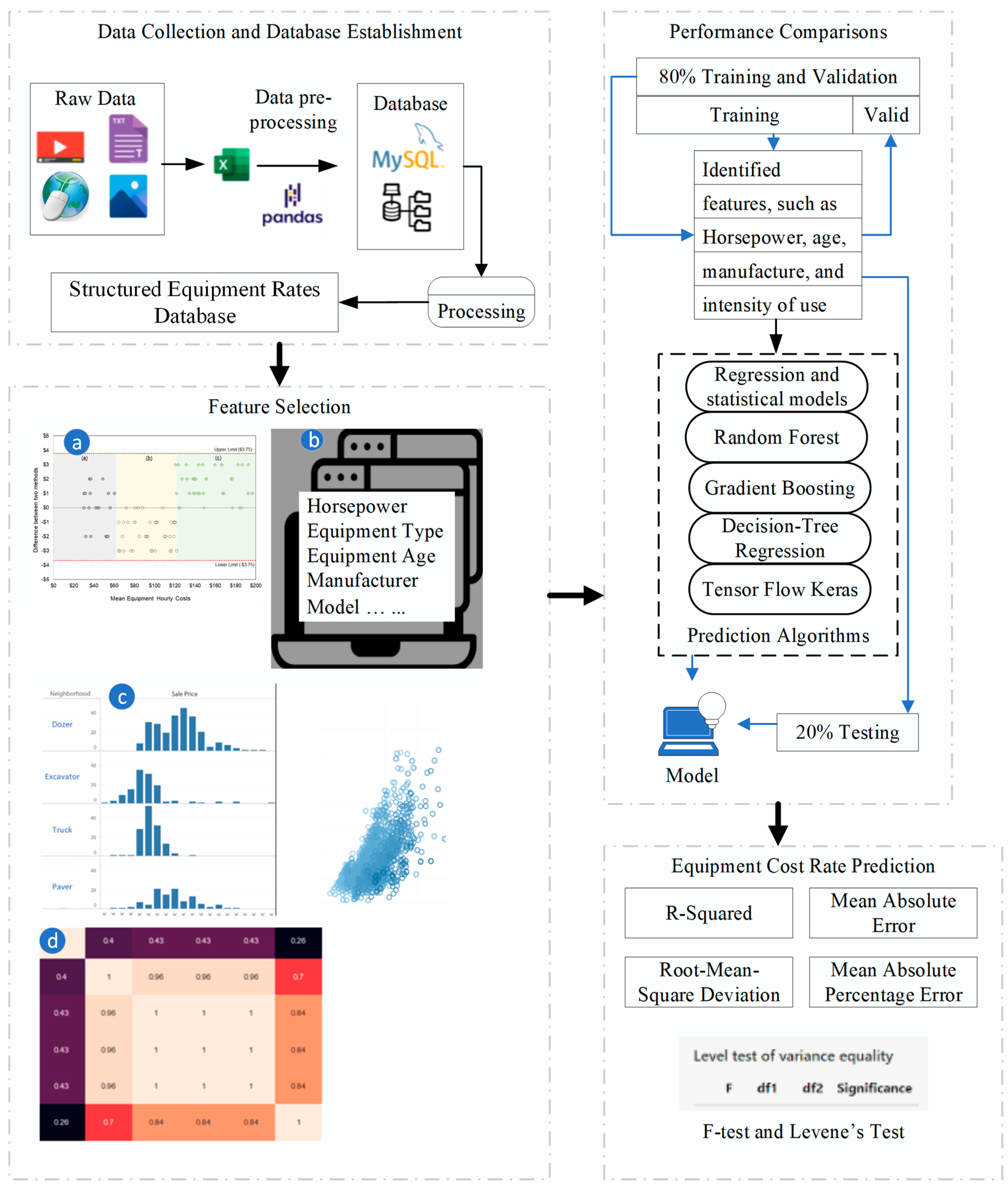
3. Research Methodology

3.1. Proposed Solution

Based on Figure 1 and Table 2, the ECR of a piece of equipment includes the ownership cost, operation cost, and other costs. The weights of the three types of costs can be obtained from training datasets using machine-learning methods. Afterward, the developed model can be implemented to predict costs using multi-dimensional data, with continuous improvements. The accuracy of the results can be compared with those in published literature using variance measurements. In this study, statistical measures like R² can help determine how well the predicted results fit the regression model that is generated from an actual dataset.

The ECR model focuses on the cost estimate, budget control, and work reimbursement of construction equipment. Based on the understanding of the equipment costs of a project (as shown in Figure 1), Equations (1)–(4) are used to calculate the ECR predictions. Appendix A and Appendix B explain the calculation of ownership costs and the estimates of hourly owning and operating costs. In these equations, the costs also include geographical difference adjustments, such as transportation distances of shipping equipment, local taxes, and weather factors. The h, i, j, and k are coefficients for the factors.

$$ECR=h\times EHRR+i\times OCR+j\times LSR+k\times Other,$$

(1)

where ECR = equipment cost rate, EHRR = equipment hourly rental rate, OCR = operating cost rate, and LSR = labor salary rate;

$$\mathit{EHRR}=\mathrm{OwningCost}=\frac{(DP-TRC)-RVR}{Hours}+Interest+Insurance+Tax+LSR,$$

(2)

where DP = delivered price to a customer (including attachments), TRC = tire replacement cost if desired, and RVR = residual value at replacement; the interest, insurance, and tax are all hourly rates; and LSR = license and storage rate.

$$OCR=UnitFuelPrice\times Consumption+PM+Tires+Undercarriage+Repair+SpecialWearItems,$$

(3)

where PM = planned maintenance = lube oil cost + filter cost + grease cost + maintenance labor, tires = $\frac{ReplacementCost}{LifeinHours}$, $Undercarriage=\left(Impact+Abrasiveness+ZFactor\right)\times BasicFactor$, and SpecialWearItems = $\sum \frac{ItemCost}{ItemLife}$.

LSR = Operator’s Hourly Wage + Fringes per hour

(4)

The data range of equipment value is from 2015 to 2022, as shown in data source #1 of Equipment Rates Database One (see DS#1 of Table 3). The equipment ages are in the range of [5,15] years, as shown in data source #2 of Table 3. The equipment types include track dozers, excavators, and trucks for building construction, as shown in data source #3 of Table 3. These equipment types are selected because they are widely used in building construction and have been studied in previous research (e.g., [10,19]). The data scope selection considers the availability of open-access databases, commonly used construction equipment types, and the contemporality of data changes due to global supply chain problems that emerged during the pandemic lockdowns. The training datasets are from Table 3. Operator salaries from publications in the FY 2015–2022 were used and the costs of equipment and fuel are from the same period.

Table 3. Data sources of Equipment Rates Database (accessed 6 September 2022).

DS	Name	Data Source (DS)
1	CalTrans	California State Transportation Agency (400 Capitol Mall Suite 2340, Sacramento, CA, USA), Labor Surcharge and Equipment Rental Rates (Effective 1 April 2021, through 31 March 2022)
2	USDA Website	Equipment Rates: https://www.fs.usda.gov/Internet/FSE_DOCUMENTS/stelprdb5247321.pdf
3	Truck and Equipment	https://www.iltruck.com/
4	Operator Salary	http://www.salary.com
5	Equipment Specs	https://www.constructionequipmentguide.com/equipment-specs-and-charts
6	AGC Equipment Cost	https://www.agc.org/sites/default/files/Files/Construction%20Markets/CM_GC_Guidelines.pdf
7	USACE Website	https://www.usace.army.mil/Cost-Engineering/EP1110-1-8/
8	U.S. EIA Website	Energy Information Administration (1000 Independence Ave., SW, Washington, DC, USA): https://www.eia.gov/petroleum/gasdiesel/ and Electric Power Monthly: https://www.eia.gov/electricity/monthly/epm_table_grapher.php?t=epmt_5_6_a
9	Alibaba Website	Heavy Construction Equipment for Sale, Rent, and Lease: https://www.alibaba.com
10	Equipment Trader	Used Heavy Construction Equipment for Sale: https://www.equipmenttrader.com/
11	Machinery Trader	(Construction) New and Used. https://www.machinerytrader.com/
12	Machinery Zone	Classified Ads for Construction Equipment. https://www.machineryzone.com/
13	U.S.A. Mascus	Used Construction and Farm Equipment. https://ar.mascus.com/
14	Iron Planet	Used Heavy Construction Equipment and Trucks for Sale. https://eu.ironplanet.com/?iprefoh=www.ironplanet.com
15	Equipment Watch	Residual Value. https://equipmentwatch.com/values-guide/
16	Bureau of Economic Analysis (BEA)	GDP estimations: https://www.bea.gov/data/gdp/gross-domestic-product
17	U.S. Census Bureau Website	https://www.census.gov/construction/c30/c30index.html

Table 3. Data sources of Equipment Rates Database (accessed 6 September 2022).

DS	Name	Data Source (DS)
1	CalTrans	California State Transportation Agency (400 Capitol Mall Suite 2340, Sacramento, CA, USA), Labor Surcharge and Equipment Rental Rates (Effective 1 April 2021, through 31 March 2022)
2	USDA Website	Equipment Rates: https://www.fs.usda.gov/Internet/FSE_DOCUMENTS/stelprdb5247321.pdf
3	Truck and Equipment	https://www.iltruck.com/
4	Operator Salary	http://www.salary.com
5	Equipment Specs	https://www.constructionequipmentguide.com/equipment-specs-and-charts
6	AGC Equipment Cost	https://www.agc.org/sites/default/files/Files/Construction%20Markets/CM_GC_Guidelines.pdf
7	USACE Website	https://www.usace.army.mil/Cost-Engineering/EP1110-1-8/
8	U.S. EIA Website	Energy Information Administration (1000 Independence Ave., SW, Washington, DC, USA): https://www.eia.gov/petroleum/gasdiesel/ and Electric Power Monthly: https://www.eia.gov/electricity/monthly/epm_table_grapher.php?t=epmt_5_6_a
9	Alibaba Website	Heavy Construction Equipment for Sale, Rent, and Lease: https://www.alibaba.com
10	Equipment Trader	Used Heavy Construction Equipment for Sale: https://www.equipmenttrader.com/
11	Machinery Trader	(Construction) New and Used. https://www.machinerytrader.com/
12	Machinery Zone	Classified Ads for Construction Equipment. https://www.machineryzone.com/
13	U.S.A. Mascus	Used Construction and Farm Equipment. https://ar.mascus.com/
14	Iron Planet	Used Heavy Construction Equipment and Trucks for Sale. https://eu.ironplanet.com/?iprefoh=www.ironplanet.com
15	Equipment Watch	Residual Value. https://equipmentwatch.com/values-guide/
16	Bureau of Economic Analysis (BEA)	GDP estimations: https://www.bea.gov/data/gdp/gross-domestic-product
17	U.S. Census Bureau Website	https://www.census.gov/construction/c30/c30index.html

The overall system design is composed of a selected frontend (i.e., user query interface) and backend software. The significant outcomes are a comprehensive understanding of which variables influence the equipment costs and how they affect ECR predictions. As [21,22] suggested, cost indices need to be updated periodically for a practical and reliable cost database. From an equipment purchase or rental perspective, the factors used in Equations (1)–(4), including maintenance and miscellaneous expenses, should be generated using some identified machine-learning and statistical methods.

The suitability of model outputs is validated through extensive statistics to understand the variance (positive or negative) between the updated hourly costs and actual costs. For example, the update of the hourly equipment rate for specific types of equipment from 2018 to 2022 can support the test of the accuracy of the updated rates by comparing them with the actual rates in 2022. In this research, a validation task is to measure the difference between the prediction results from the system and the outcomes from a commercially available database, as well as a few publications.

Specifically, the TVM of equipment costs, especially in the current economic crisis, can be reflected by machine-learning models [10,18,19]. Figure 2 shows two conceptual scenarios of time series data, where the variable x represents time and the variable y represents the TVM of equipment costs.

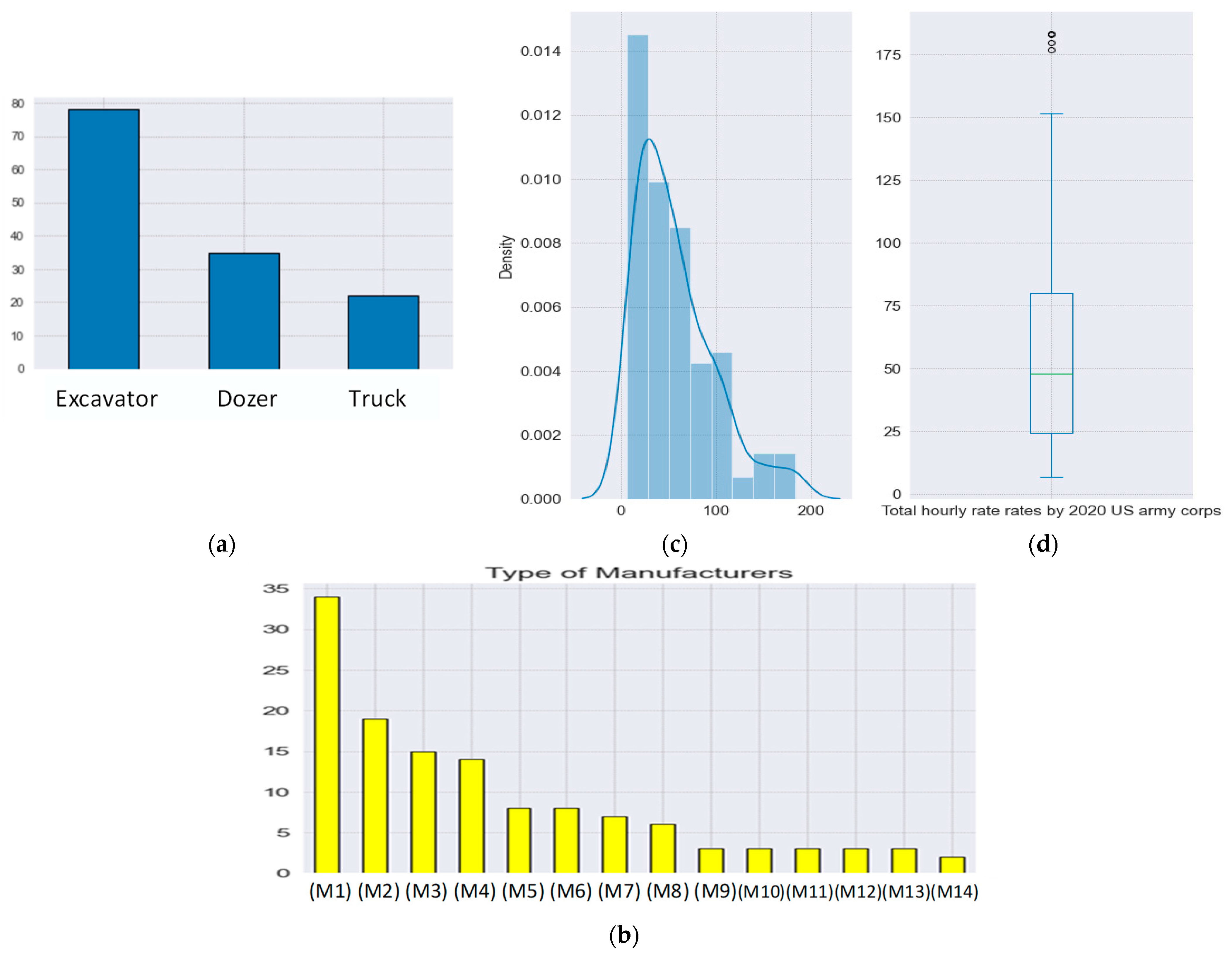
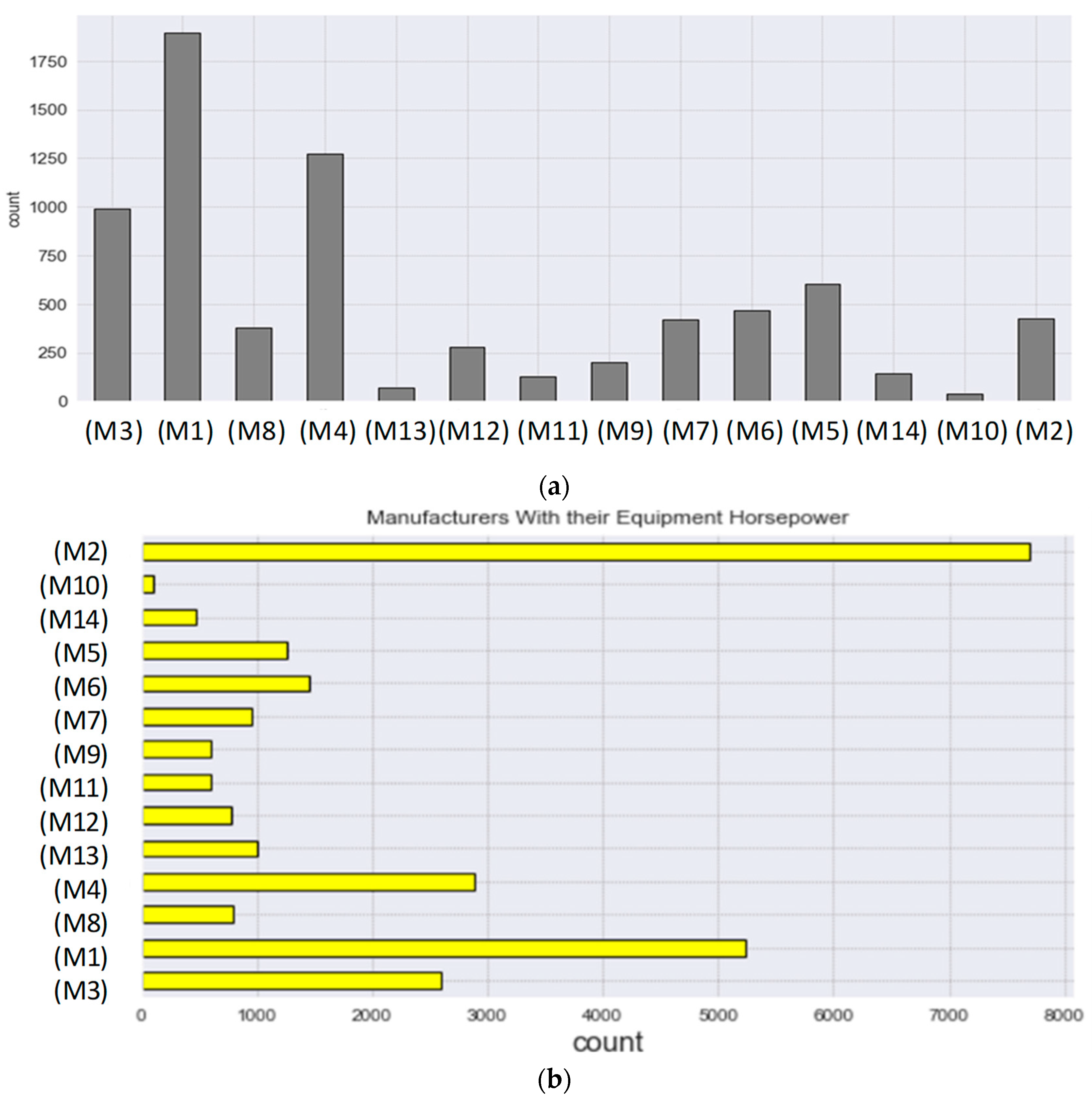
3.2. Data Collection and Model Development

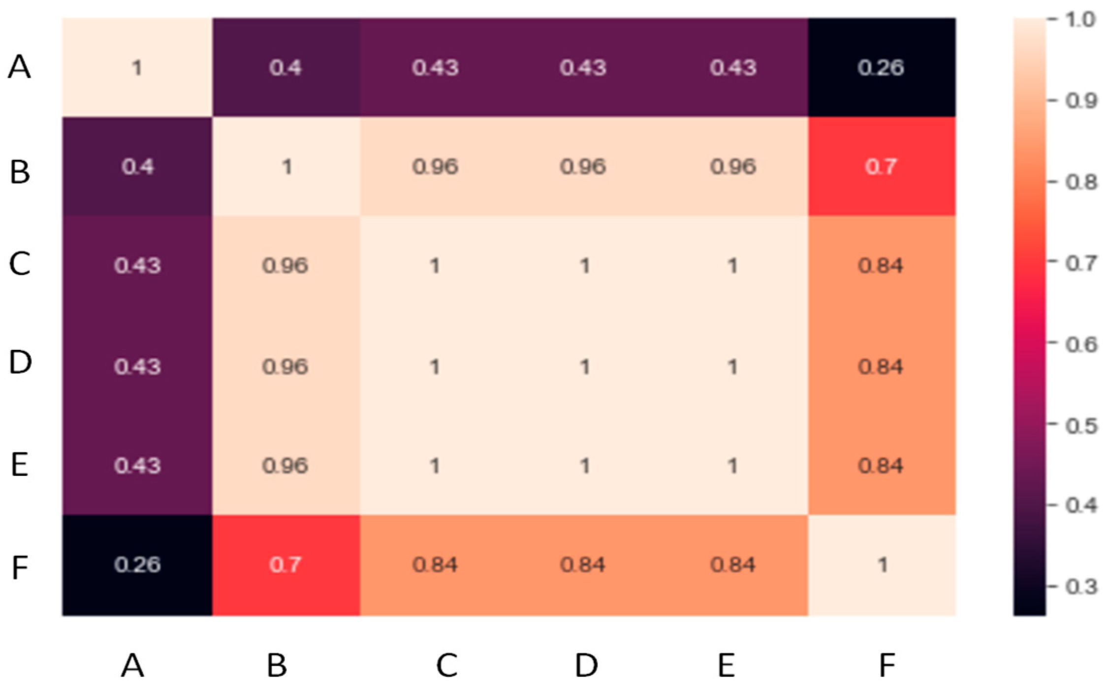
This study assumes that equipment cost is affected by the availability of equipment. Hence, the machine-learning-based prediction model needs to rely on more recent data to sustain its dynamic features and improve the accuracy and reliability of forecasts [23]. Figure 3 shows the details about desired data, related participants, and data-gathering methods.

First, the cost data was extracted from the open-access databases (see Table 3 for details). Because the data collected was in a combination of structured and unstructured formats, it was transformed into the desired structures and then cleaned by removing empty and incorrect datasets. The next step was to explore and examine the pre-processed data. The agreement charts of the identified equipment types were analyzed for pattern recognition. As [24,25] suggested, a Bland–Altman procedure or equivalent was applied to develop the limits of agreement. Such a method usually calculates the mean difference as two times the standard deviation (1.96 × SD to be precise), which represents the 95% limits of agreement. In other words, this mean difference is expected to include 95% of the differences (also known as bias between observations and estimates) between the two measurement methods. An example is shown in Figure 4, where the mean equipment hourly costs are on the x-axis and the differences between the two methods are on the y-axis. An ideal data pattern is shown in Zone (a) of Figure 4. Zone (b) in the middle of Figure 4 shows that the method produced higher costs than the commercial database for a particular hourly cost range (USD 60–USD 120), whereas Zone (c) shows an opposite trend. Compared to Zone (a), if data shows trends like the ones in Zones (b) and (c), adjustments to costing equations should be made. As shown in Figure 4, the y-axis displays the differences between the hourly costs derived from the two methods. Figure 4, Zone (a) shows that, at a 95% confidence level, the limit of agreement is USD −3.75 to USD +3.75. Hence, the hourly costs of the method are within USD 3.75 higher or lower than the commercial database.

Figure 4 also shows how to handle risks and uncertainties. Risk elements and uncertainties can affect equipment costs and are handled in the model. Particularly, confidence intervals are used to indicate the level of certainty (or uncertainty) of the predictions or outputs the model has generated. The case in Figure 4 has a 95% confidence interval.

The software tools used in this process included Python^® software (v3.10.8, 64-bit) to implement the calculation and prediction models, JetBrains Pycharm Community Edition^® (v2022.2.4, build 222.459.20) for a cross-platform integrated development environment, and Python library packages such as Pandas (v1.5.1) to design and implement database structures, as well as accomplish exploratory data analysis. Python was used as a backend programming language to support calculating the equipment cost for the given user inputs. Within Python, the SciKitLearn and TensorFlow machine-learning libraries were used to extract the required data from the database, and apply specific models to estimate various cost components and plug them into an equipment costing equation.

Figure 5 shows the system structure and its four major stages, namely, data collection and database establishment, feature selection, performance comparisons, and equipment cost rate prediction. The arrows in Figure 5 show the workflow of system implementation. In the feature-selection stage element (a) represents the determination of the upper and lower boundaries of the independent variables; element (b) represents the features in Table 2; and element (c) represents backward elimination, which is a feature-selection technique when creating a machine-learning model. The elimination process removes the insignificant features that have been decided by comparing their influences on the dependent variable, i.e., the prediction variable).

3.3. Comparison

The Performance Comparisons stage of Figure 5 supports the model implemented for the prediction of ECR. To construct the model, a rules-based technique, regression and statistical models, and machine-learning algorithms were integrated. This strategy follows the 80–20 rule, namely 80% of the collected data is used for training and validation purposes, and 20% of the collected data is for testing purposes. In this component, data mining techniques like K-means and SVM were implemented. K-means selects a centroid for each cluster, e.g., the most representative model of trucks in construction projects, while the SVM-supervised machine-learning clustering method was used to classify data into two distinctive classes. The data mining methods are combined with a variety of algorithms, including an autoregressive tree, multivariate linear regression, and artificial neural networks. Based on the literature review, several machine-learning and deep-learning techniques, including multiple linear regression, K-nearest neighbors (KNN), decision trees, and naive Bayes, were evaluated. Then, regression and statistical models, random forest, gradient boosting, decision-tree regression, and SVM algorithms were selected and implemented. The selection was mainly based on the 80% or better prediction accuracy.

Four indicators were then calculated to examine the performances of predictions, including R², root-mean-square error (RMSE), mean absolute error (MAE), and mean absolute percentage error (MAPE). Equations (5)–(8) explain the calculation details. The R² indicator is widely used to measure the strength of the relationship between the prediction of a linear model and its dependent variable and indicates how well a regression model describes observed data. The main purpose of using the R² indicator is to avoid overfitting a machine-learning model, thus preventing the model from picking up noises. Nevertheless, the value criterion of R² depends on the context. In this study, the R² indicator is set to be 0.8 or higher [26].

$$R^2=\frac{Varianceexplainedbythemodel}{Totalvariance}$$

(5)

$$RMSE=\sqrt{\frac{{\sum }_{i=1}^N{(x_i-\widehat{x_i})}^2}{N}},$$

(6)

where i is a variable, N = number of non-missing data points, $x_i$ = actual observations time series, and $\widehat{x_i}$ = estimated time series.

$$MAE=\frac{{\sum }_{i=1}^N\left|\widehat{x_i}-x_i\right|}{N}$$

(7)

$$MAPE=\frac{1}{N}{\sum }_{i=1}^N\frac{\left|\widehat{x_i}-x_i\right|}{x_i}$$

(8)

3.4. Development of ECR Model

The model development process in this research involves planning and analysis, database structure design, data preparation, function development using different techniques, system integration, and testing. After testing the prediction functions, the model was evaluated by examining the prediction outcomes and their correctness. In addition to the evaluation, the validity and effectiveness of the data mining methods were examined.

The developed system estimates equipment costs using the developed costing model shown in Figure 1. However, the user inputs themselves are not direct values that can be plugged into the equation. For instance, if the user enters the equipment type as a two-year medium-duty truck, then the system will search the database to identify the information related to the medium-duty truck and generate the required values (fuel consumption, tire costs, etc.) to plug into the costing model. While the system can extract some costs directly from the database, other costs need processing. Occasionally, if the equipment is not listed in the database or if the equipment is too old, the system needs to predict the most reasonable costs. Therefore, this task focuses on developing cost-prediction models using advanced data analytics.

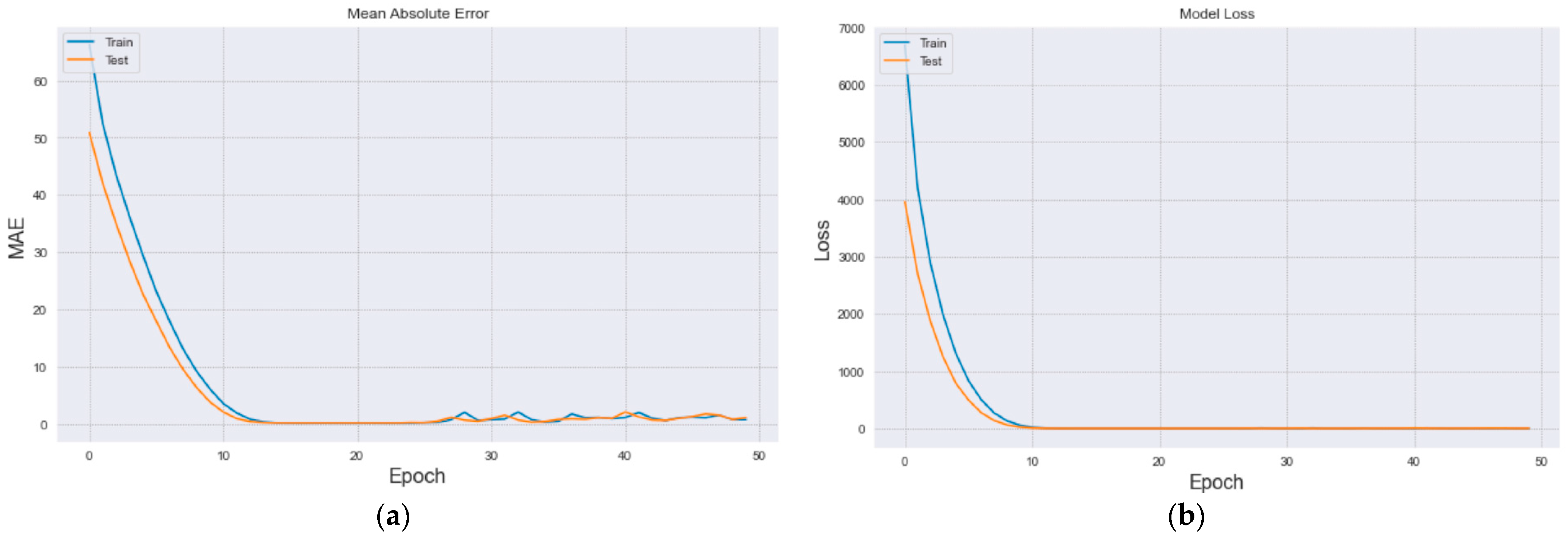
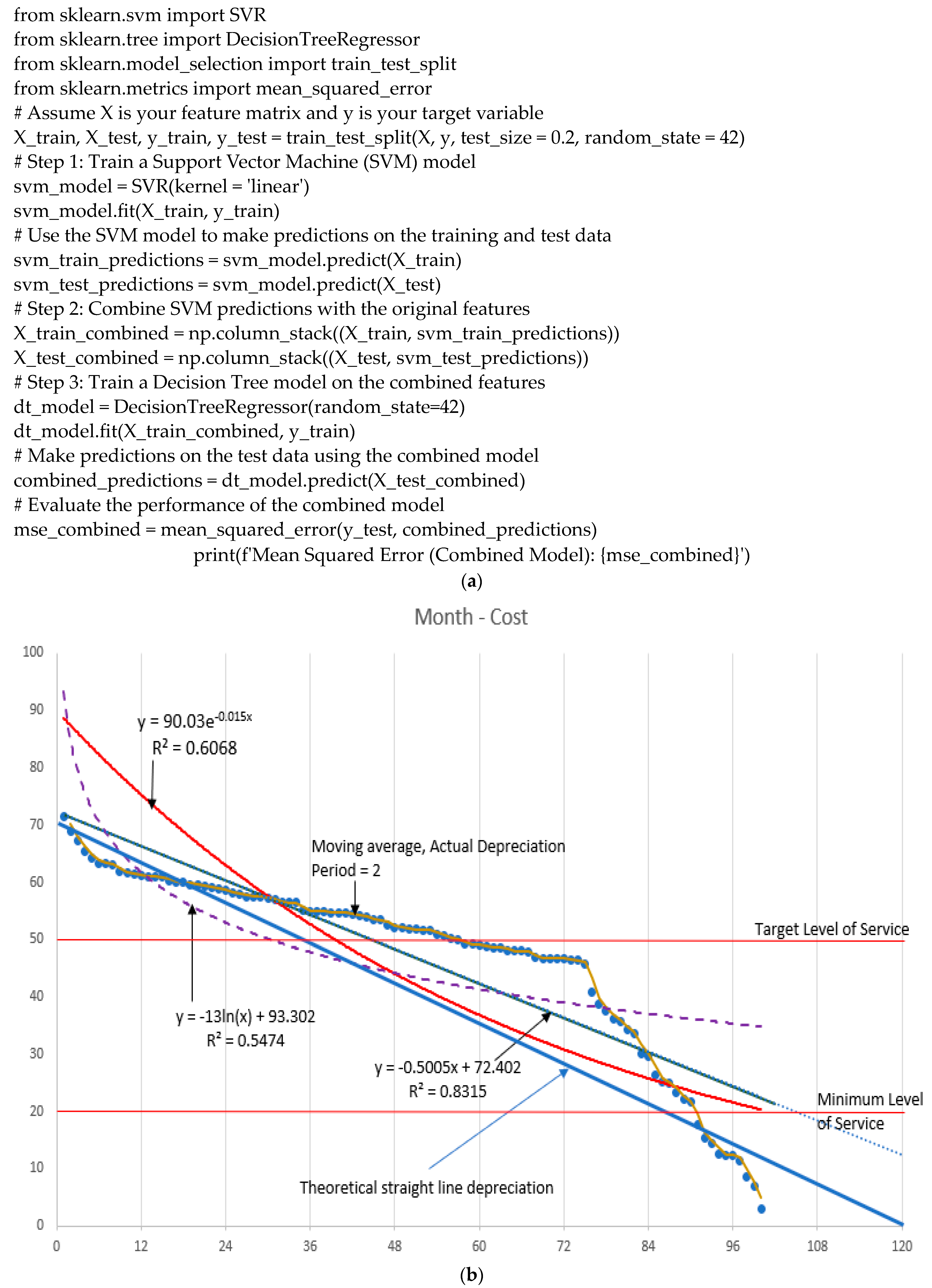
4. Analysis and Discussion

Figure 6a–d describe the collected data, their features, and the analysis results. Figure 6a shows that the dataset has 78 types of excavators, 35 types of track dozers, and 22 types of trucks. Figure 6b shows equipment manufacturers. The Figure 6c distribution plot and Figure 6d boxplot are used to check for outliers. During the training, testing, modeling, and cross-validation processes, the datasets were thoroughly investigated using statistical and machine-learning algorithms.

Figure 7a indicates that three types of equipment (excavators, track dozers, and trucks) are selected for the study of fuel costs. Figure 7c shows that three distinctive bars representing equipment clusters are taller than the rest. Figure 7b shows that some manufacturers have wider scopes of ECR than others. Figure 7d shows a moderate linear regression. Figure 8 shows the results of the attribute correlation matrix, where A is equipment horsepower; B is value in 2015; C is total hourly rate specified by 2018 USACE; D is total hourly rate specified by 2020 USACE; E is total hourly rate specified by 2020 IDOT Procedure; and F is fuel cost.

Figure 9a shows the manufacturer data. The testing dataset has the ECR data for excavators, track dozers, and trucks because they are commonly used by small- and medium-sized contractors in highway projects. Figure 9b comprises the manufacturers with their equipment horsepower.

This research implemented and compared four machine-learning-based methods: random forest, gradient boosting, decision-tree regression, and SVM. TensorFlow Keras (TFK) is an open-source Python library and has features like auto-differentiation to calculate the gradient vector of a model for each parameter, eager execution to examine and augment data at each line of code, and training neural networks for optimization purposes. In this study, the TFK library provides feature scaling and data normalization functions to standardize the different scales and ranges of data features of SVM functions for the modified decision-tree model. The epoch of machine learning is 10 (see Figure 10 for details).

The accuracy of the algorithms was evaluated and compared using four performance indicators, namely MAE, MSE, MAPE, and R². The data collected indicated that both the USACE and the IDOT use linear models for ECR calculations. Traditional statistical methods have difficulties in creating precise models for predicting the residual values of construction equipment [13,14]. Even though machine learning has been widely implemented in various areas for prediction, many owners and engineers in the construction industry are still using linear regressions to predict ECRs. Hence, in this research, linear regressions were included in the comparisons (see

Table 4. Performance comparison.

	Linear Regression	Random Forest	Gradient Boosting	Decision-Tree Regression	Modified Decision Tree (MDT) with SVM
R2	1.00	0.99	1.00	0.97	1.00
RMSE	0.00	3.37	2.62	2.62	1.73
MAE	0.00	1.95	1.32	1.32	1.38
MAPE	0.00	0.0300	0.0200	0.0200	0.0198

). Furthermore, gradient-boosting and decision-tree methods were implemented. A modified decision-tree regression model (MDT) with SVM was also established in this study for ECR prediction (see the figure in Appendix C for further details). The MDT-SVM model has the greatest prediction accuracy of 1.00 in R² and 1.73 in RMSE indicators (see Table 4 for performance comparison). The method also has high accuracy in the MAE and MAPE indicators. Shehadeh et al. [10] indicated that the manufacturing countries and intensity of use factors had more influences than others. The results from this research suggested that horsepower and manufacturer have more influence than other factors. As shown in Table 4, the MDT-SVM model (see also Figure 11a) has outperformed the decision-tree method in R² (2%), RMSE (33.97%), and MAPE (1%). The decision-tree method has better performance than the MDT-SVM model in MAE (4.55%).

Both the decision-tree method and the MDT-SVM model are acceptable in prediction accuracies. However, a decision-tree model frequently has some substantial limitations, such as human intervention, long pre-processing time, and laborious updates. One significant concern is the perceived “black-box” nature of these models, which may overlook crucial elements that experienced managers bring to the decision-making process (see Table 1). One solution is to synthesize the findings of this research with other literature. Akinosho et al. [27] studied the “black-box” challenge in the implementation of deep learning in the construction industry and suggested that plotting a model’s response and partial dependency (PD) was a promising solution. In this study, Figure 7 presents the model response and Figure 8 shows the result of PD.

Another way to improve the interpretation of the results from machine-learning models is to incorporate the participation of managers (i.e., intuition, experience, sensation, experience, belief, knowledge, etc.) Nine factors were identified to affect cost estimate accuracy: the market’s state, the estimating team’s experience level, site conditions, labor and equipment required, transportation problems, periodical payments, availability of productivity standards, availability of power and water in site, and availability of management and finance plans [28]. In particular, the site conditions of a project can affect the horsepower and manufacturer selection of equipment. The findings of this study confirm that the data and information on horsepower and manufacturer selections of equipment are crucial to support decisions in cost estimates.

This research found that the equipment costs associated with public construction projects tend to be linear, while the construction equipment costs associated with private sectors are nonlinear. When using the datasets (DS# 1, 2, 7, 8, 16, and 17; see Table 3), the results from linear correlations have better prediction accuracies than the nonlinear correlations. When using the rest of the datasets in Table 3, the results from nonlinear correlations are better. Therefore, using this feature to train the decision tree can make prediction more accurate compared to using the decision-tree method alone.

Figure 11b shows the trend patterns of a heavy-duty track about its residual values and service costs. The datasets of this figure are from a commercial equipment rental company and Table 3. The trends and patterns are generated from the MDT-SVM model. The results can help engineers and managers understand the equipment value’s actual depreciation, predict its residual values, and identify the minimum level of service. For example, for a USD 70,000 device with a 10-year (120-month) service life (as suggested by [29]), multiple regression models can be used to describe the residual value of the device. According to straight-line depreciation, the device should be repaired or replaced in Month 90 to bring it back to the target level of service. From Month 76 to Month 90, the device experiences fast depreciation.

5. Conclusions

In this study, a machine-learning-based prediction method for ECR was developed. The performance comparison of this developed MDT-SVM model with linear regression and other machine-learning-based models was performed. The results showed that the MDT-SVM model has better accuracy (3–33.97%) in equipment cost predictions for building construction. The model can accommodate market changes to establish equipment cost rates, while linear regression fails to fit complex variations. The prediction model can provide automatic assistance and suggestions as well. It has relatively better performance than decision-tree regression in reducing prediction errors. It provides the best estimate at a given time by considering (1) horsepower, (2) manufacturers’ inputs, (3) residual value, and (4) fuel cost. The research results can provide improved decision support for industry professionals to calculate and estimate equipment costs.

The research approach involves a comprehensive literature review, advanced data analytics, and statistical methods. The developed database structure provides reasonable rates for a multitude of construction equipment. Implementing the prediction model to create cost predictions can empower the construction industry by compensating reasonable equipment costs to contractors. It benefits construction companies by saving on commercial database subscription costs. This research can give small- and medium-sized construction companies the ability to reduce costs and grow business.

During the study, it was noticed that the equipment cost scheme needs to go through a cost updating process at least once a year, to bring the equipment costs closer to actual costs. Future research should help to decide the appropriate time for updating equipment costs. For example, when the commonly used equipment of building projects, such as excavators and trucks, has significant discrepancies between the rental costs and the residual values calculated by a straight-line depreciation method, industry professionals should consider adjusting the corresponding equipment costs.

In conclusion, machine-learning technologies offer valuable insights. Yet, their integration into decision-making processes for equipment selection and maintenance should be complemented by the expertise, intuition, and experience of human managers. A collaborative strategy that integrates the strengths of machine learning with the sophisticated understanding of industry professionals is likely to result in more informed and robust decisions, enhancing the overall efficiency and success of construction projects.

References

1. Shaurette, M. Higher Hourly Cost Compensation for Heavy Equipment Used In Demolition Activity. Int. J. Constr. Educ. Res. 2015, 11, 280–291. [Google Scholar] [CrossRef]
2. EquipmentWatch. Available online: https://equipmentwatch.com/ (accessed on 6 February 2023).
3. Illinois Department of Transportation Annual Report. 2021. Available online: https://idot.illinois.gov/about-idot/our-story/performance/reports/annual-reports.html (accessed on 20 April 2022).
4. Jorge, J.E.; Herbsman, Z. Determination of Construction Equipment Rental Rates in Force Account Operations for Federal and State Government Agencies. In Proceedings of the Transportation Research Record, Washington, DC, USA, 5–7 January 1989; Volume 1234, pp. 74–83. [Google Scholar]
5. The Schedule of Average Annual Equipment Ownership Expense (SOAAEOE). Available online: https://idot.illinois.gov/transportation-system/local-transportation-partners/county-engineers-and-local-public-agencies/lpa-project-development-and-implementation/policy-and-procedures/schedule-avg.html (accessed on 20 April 2022).
6. Slobodnyak, I.; Sidorov, A. Time Value of Money Application for the Asymmetric Distribution of Payments and Facts of Economic Life. J. Risk Financ. Manag. 2022, 15, 573. [Google Scholar] [CrossRef]
7. AGC Contractors Equipment Cost Guide. Available online: https://www.agc.org/sites/default/files/Files/Construction%20Markets/CM_GC_Guidelines.pdf (accessed on 30 March 2022).
8. Labor Surcharge and Equipment Rental Rates. Division of Construction, Department of Transportation, California State Transportation Agency, State of California. Available online: https://dot.ca.gov/programs/construction/equipment-rental-rates-and-labor-surcharge (accessed on 6 February 2023).
9. CAT Rental: How Much Does It Cost to Rent Heavy Equipment? Available online: https://www.catrentalstore.com/en_US/blog/cost-to-rent-heavy-equipment.html (accessed on 13 April 2022).
10. Shehadeh, A.; Alshboul, O.; Al Mamlook, R.E.; Hamedat, O. Machine Learning Models for Predicting the Residual Value of Heavy Construction Equipment: An Evaluation of Modified Decision Tree, LightGBM, and XGBoost regression. Autom. Constr. 2021, 129, 103827. [Google Scholar] [CrossRef]
11. Xie, H.; Shi, W.; Issa, R.R.; Guo, X.; Shi, Y.; Liu, X. Machine Learning of Concrete Temperature Development for Quality Control of Field Curing. J. Comput. Civ. Eng. 2020, 34, 04020031. [Google Scholar] [CrossRef]
12. Neloy, A.A.; Haque, H.S.; Ul Islam, M.M. Ensemble Learning Based Rental Apartment Price Prediction Model by Categorical Features Factoring. In Proceedings of the 2019 11th International Conference on Machine Learning and Computing, Zhuhai, China, 22–24 February 2019; pp. 350–356. [Google Scholar]
13. Li, Y.; Wang, S.; Ma, Y.; Pan, Q.; Cambria, E. Popularity Prediction on Vacation Rental Websites. J. Neurocomputing 2020, 412, 372–380. [Google Scholar] [CrossRef]
14. Abed, Y.G.; Hasan, T.M.; Zehawi, R.N. Cost Prediction for Roads Construction using Machine Learning Models. Int. J. Electr. Comput. Eng. Syst. 2022, 13, 927–936. [Google Scholar]
15. Heidari, M.; Zad, S.; Rafatirad, S. Ensemble of Supervised and Unsupervised Learning Models to Predict a Profitable Business Decision. In Proceedings of the IEEE International IOT, Electronics and Mechatronics Conference (IEMTRONICS), Toronto, ON, Canada, 21–24 April 2021; pp. 1–6. [Google Scholar]
16. Wang, W.; Pan, C. Collectively Learned Multi-Level Spatial Embeddings for Residential Rental Price Prediction. In Proceedings of the IEEE International Conference on Big Data (Big Data), Orlando, FL, USA, 15–18 December 2021; pp. 274–283. [Google Scholar]
17. Heidari, M.; Rafatirad, S. Bidirectional Transformer Based on Online Text-Based Information to Implement Convolutional Neural Network Model for Secure Business Investment. In Proceedings of the IEEE International Symposium on Technology and Society (ISTAS), Tempe, AZ, USA, 12–15 November 2020; pp. 322–329. [Google Scholar]
18. Feng, Y.; Wang, S. A Forecast for Bicycle Rental Demand Based on Random Forests and Multiple Linear Regression. In Proceedings of the IEEE/ACIS 16th International Conference on Computer and Information Science (ICIS), Wuhan, China, 24–26 May 2017; pp. 101–105. [Google Scholar]
19. Alshboul, O.; Shehadeh, A.; Al-Kasasbeh, M.; Al Mamlook, R.E.; Halalsheh, N.; Alkasasbeh, M. Deep and Machine Learning Approaches for Forecasting the Residual Value of Heavy Construction Equipment: A Management Decision Support Model. J. Eng. Constr. Archit. Manag. 2021, 29, 4153–4176. [Google Scholar] [CrossRef]
20. Supervised vs. Unsupervised Learning; What’s the Difference? IBM Blog. Available online: https://www.ibm.com/cloud/blog/supervised-vs-unsupervised-learning (accessed on 17 November 2022).
21. Seresht, N.G.; Fayek, A.R. Dynamic Modeling of Multifactor Construction Productivity for Equipment-Intensive Activities. J. Constr. Eng. Manag. 2018, 144, 04018091. [Google Scholar] [CrossRef]
22. Milošević, I.; Kovačević, M.; Petronijević, P. Estimating Residual Value of Heavy Construction Equipment Using Ensemble Learning. J. Constr. Eng. Manag. 2021, 147, 04021073. [Google Scholar] [CrossRef]
23. Baduge, S.K.; Thilakarathna, S.; Perera, J.S.; Arashpour, M.; Sharafi, P.; Teodosio, B.; Shringi, A.; Mendis, P. Artificial Intelligence and Smart Vision for Building and Construction 4.0: Machine and Deep Learning Methods and Applications. Autom. Constr. 2022, 141, 104440. [Google Scholar] [CrossRef]
24. Khalaf, T.Z.; Çağlar, H.; Çağlar, A.; Hanoon, A.N. Particle Swarm Optimization Based Approach for Estimation of Costs and Duration of Construction Projects. J. Civ. Eng. 2020, 6, 384–401. [Google Scholar] [CrossRef]
25. Lee, J.; Matsumura, K.; Yamakoshi, K.I.; Rolfe, P.; Tanaka, S.; Yamakoshi, T. Comparison between red, green and blue light reflection photoplethysmography for heart rate monitoring during motion. In Proceedings of the 35th Annual International Conference of the IEEE Engineering in Medicine and Biology Society (EMBC), Osaka, Japan, 3–7 July 2013; pp. 1724–1727. [Google Scholar]
26. Chicco, D.; Warrens, M.J.; Jurman, G. The Coefficient of Determination R-squared Is more Informative than SMAPE, MAE, MAPE, MSE and RMSE in Regression Analysis Evaluation. PeerJ Comput. Sci. 2021, 7, e623. [Google Scholar] [CrossRef] [PubMed]
27. Akinosho, T.D.; Oyedele, L.O.; Bilal, M.; Ajayi, A.O.; Delgado, M.D.; Akinade, O.O.; Ahmed, A.A. Deep learning in the construction industry: A review of present status and future innovations. J. Build. Eng. 2020, 32, 101827. [Google Scholar] [CrossRef]
28. Sayed, M.; Abdel-Hamid, M.; El-Dash, K. Improving cost estimation in construction projects. Int. J. Constr. Manag. 2023, 23, 135–143. [Google Scholar] [CrossRef]
29. USACE. EP1110-1-8 Construction Equipment Ownership and Operating Expense Schedule. Available online: https://www.usace.army.mil/Cost-Engineering/EP1110-1-8/ (accessed on 30 March 2022).
Figure 1. Typical equipment cost components.
Buildings 14 00436 g001
Figure 2. Conceptual representations of TVM: (a) linear relationship; (b) nonlinear relationship with inflation.
Buildings 14 00436 g002
Figure 3. Planned data collection types, sources, and data collection methods. (Caterpillar, Inc., Irving, TX, USA; Bridgestone, Nashville, TN, USA; State Farm, Bloomington, IN, USA).
Buildings 14 00436 g003
Figure 4. Example showing the comparisons of two methods with marked upper and lower limits of agreement between methods.
Buildings 14 00436 g004
Figure 5. System structure. (a) boundary determination, (b) features, (c) feature selection, (d) attribute correlation.
Buildings 14 00436 g005
Figure 6. Features and analysis of the collected data. (a) Each equipment type with its count values; (b) Type of manufacturers; (c) distribution plot to check outliers; (d) box plot to check outliers.
Buildings 14 00436 g006
Figure 7. Effects of (a) fuel cost, (b) manufacturer, (c) horsepower, and (d) residual value on the hourly cost rate of the equipment.
Buildings 14 00436 g007
Figure 8. Attribute correlation matrix.
Buildings 14 00436 g008
Figure 9. 2020 USACE data for testing prediction results. (a) Manufacturer’s total hourly rate (data from 2020 US Army Corps); (b) Manufacturer’s equipment horsepower.
Buildings 14 00436 g009
Figure 10. Epoch calculation. (a) MAE; (b) Model loss.
Buildings 14 00436 g010
Figure 11. (a) Pseudocode of MDT-SVM and (b) depreciation models.
Buildings 14 00436 g011