Abstract
Due to their roles as efficient lateral force-resisting systems, reinforced concrete shear walls exert a tremendous degree of influence on the overall seismic performance of buildings. The ability to predict the boundary transverse reinforcement of shear walls is critical to the seismic design process, as well as in the overall evaluation and retrofitting of existing buildings. Contemporary empirical models attain low predictive accuracy, with an inability to capture nonlinearity between boundary transverse reinforcement and different influencing variables. This study proposes a boundary transverse reinforcement prediction model for shear walls with boundary elements based on the demand of ductility. Using the extreme gradient boosting machine learning algorithm and 501 samples, some 52 input variables are considered, and a subset with six features is selected, monitored, and analyzed using both internal methods (gain and cover) and external methods. The results () display superior predictive capacity compared with existing models. Interpretation and error analysis are performed. Safety analysis is conducted to obtain references for use in practical engineering. Overall, this study presents a more accurate tool for use in seismic design and provides references for the evaluation and retrofitting of existing buildings. Our contributions hold significant implications for enhancing the safety and resilience of reinforced concrete structures.
1. Introduction
1.1. Boundary Transverse Reinforcement of Reinforced Concrete Shear Walls
Reinforced concrete (RC) shear walls, utilizing boundary elements (BEs) as the primary anti-lateral force systems to cope with seismic load, are designed to provide significant lateral strength and stiffness. Design methods have been proposed and improved for RC shear walls with BEs, and experiments investigating their seismic performances have been designed and discussed [1,2,3,4]. Among these elements, ductility has been proven to be a significant design indicator of RC shear walls with BEs, due to its contributions during moderate earthquakes or rare earthquakes, events that can result in the failure and collapse of the structures. The transverse reinforcement of boundary elements exerts positive influence on ductility, enhancing the ultimate compressive strain of concrete in the potential plastic hinge zone [5,6].
Over the preceding several decades, numerous researchers have proposed boundary transverse reinforcement prediction models via theoretical derivation and verified their findings against experimental results related to different ductility demand indicators. Qian et al. [7] proposed an empirical model based on the required displacement angle for rectangular walls or I-shaped and T-shaped walls, integrating parameters including web length, wall height, and the relative height of the compressed zone. Ma et al. [8] established an empirical model based on the required plastic hinge rotation, considering the relative height of the compressed zone, seismic grades, axial load ratio, and the ultimate compressive strain requirements of the concrete at the edges of shear walls. Huang et al. [9] developed a calculation equation based on the damage index of walls, incorporating aspect ratio, axial load ratio, ultimate displacement angle, and the characteristic value of distributed reinforcement.
Based on the Chinese Code for the design of concrete structures [10], the boundary transverse reinforcement of RC shear walls is calculated via the table form, where the transverse reinforcement characteristic value () is given according to the axis load ratio under different seismic grades and seismic precautionary intensities. However, experimental results and seismic damage have illustrated that the current code does not quantitatively establish the relationship between boundary transverse reinforcement and the ductility demand of RC shear walls under different seismic grades. Therefore, ductility remains unknown when determined based on such semi-empirical and semi-theoretical design methods. This causes issues for the seismic design of new buildings, as well as the evaluation and retrofit of existed buildings. With increased interest in performance-based earthquake engineering, contemporary design methods are not capable of expressing the relationship between ductility demand and transverse reinforcement. Quantitative equations from other countries, including the 2019 version of ACI 319 (ACI Committee 318 2019) [11], Eurocode 8 (2004) [12], and NZS 3101-1 (2006) [13], are established based on mechanical analysis and related experimental studies considering various factors. Lu et al. [14,15] established two prediction models based on a quantitative ductility-based method and quantitative drift-based approach, referring to codes used in New Zealand and America, respectively. It is possible to increase the accuracy of the two models by considering the failure caused by steel yielding and concrete being crushed simultaneously.
As summarized above, traditional approaches to the boundary transverse reinforcement of shear walls are available. However, some crucial problems must be solved. In the first instance (1), we must address the lack of a more advanced model to establish quantitative relationship between boundary transverse reinforcement and the ductility demands of RC shear walls, as determined based on the development of construction and latest experimental data. Some of the methods remain established, and some formulas are still based on lower-strength experimental data. Secondly (2), we must address the unreliability of more applicable tools for the performance-based design or evaluation of buildings in large-scale engineering programs. Applicability cannot be guaranteed due to the large amount of missing data with higher axial load ratio [9] and various cross-sectional forms. We must (3) rectify the inability to capture the relationship between variables, e.g., the impact of transverse reinforcement on the final deformation. This failure occurs because numerical simulations of real-world scenarios invariably simplify or overlook certain key details [8], hindering the resolution of quantitative relationships. The final factors in need of remedying include (4) the unexpected level of accuracy and efficiency of prediction because of mechanical assumptions and considerable prerequisites, (5) the restriction of computing and analysis ability based on simple linear functions [7], or even table-form interpolation [10]. Thus, alternative models require exploration. The design and analysis of RC shear walls with BEs necessitate a more thorough consideration of factors under real load conditions and the accurate extraction of patterns from experimental data. We must develop models with stronger generalization capability based on the combination of recent and historical experimental data.
1.2. Machine Learning Performance Studies on Reinforced Concrete Shear Walls
The application of machine learning is relevant in connection with real problems and intrinsic causes [16,17]. Recent advancements in machine learning (ML) methods have produced a paradigm shift in the analysis and design of RC shear walls, as researchers seek to address existing flaws in traditional methods. The potential of performance prediction using ML methods has been underscored by several studies [18,19,20] demonstrating its superiority in handling complex data.
For simple issues in RC shear walls, such as bearing capacity prediction in the positive cross-section, traditional studies have achieved considerable accuracy. Thus, current machine learning research is primarily focused on the exploration of more complex issues involving physical, geometric, or material nonlinearity, such as backbone curves, ultimate deformation, and the energy dissipation capacity of shear walls. These issue can be categorized into several aspects, which are summarized in part as follows: (1) failure mode recognition and prediction [21,22,23,24,25]: identifying and predicting the failure modes of shear walls; (2) capacity prediction (often shear capacity) [26,27,28,29,30,31]: forecasting the load-carrying capacity of shear walls, predominantly shear capacity; (3) deformation capacity prediction [32,33]: estimating the deformation capacity of shear walls; (4) energy dissipation capacity prediction [34,35,36,37]: anticipating energy dissipation capacity, hysteresis curves, equivalent damping ratios, and related aspects. Some studies amalgamate predictions of shear wall performance [26] (failure modes, shear capacity, and deformation capacity), utilizing existing models to assist with shear wall design and the establishment of user-friendly platforms [30]. These studies have proved that ML models excel in (1) handling data with strong computing power; (2) effectively capturing the nonlinear relationships between input variables and output variables using statistical methods and with techniques based on ensemble algorithms [32]; and (3) offering a promising alternative for accurate prediction compared with empirical methods [37].
The prediction of the boundary transverse reinforcement of shear walls with BEs is related to regression problems such as deformation capacity prediction, which also involves nonlinear performance under a seismic load. As ML methods show the potential of accuracy and applicability in other ML studies of RC shear walls, they may offer novel horizons in the prediction of boundary transverse reinforcement. However, no such prediction model has been developed and explored using ML methods.
On this basis, our study aims to bridge the gaps in knowledge by developing a robust prediction model through ML algorithms. The purpose of doing so is to explore and address the following needs: (1) Develop a more precise quantitative model that links the ductility demand to the need for transverse reinforcement, thus helping to improve the seismic performance of shear walls. (2) Expand applicability and advancement. Collect the latest high-quality and representative experimental data on shear walls, covering a wider range of types to enhance credibility. (3) Integrate domain knowledge with machine learning methods in order to consolidate existing research parameters, combine them with new parameters for analysis, capture nonlinear relationships, and uncover latent patterns within subtle data relationships.
In our research, the data set of 501 samples with transverse reinforcement in the boundary elements is established and checked cautiously for the purpose of building ML models. Feature engineering is implemented in order to investigate and select the feature subset with the minimal but most representative input variables. Statistical indicators are used to evaluate the performance of ML models and choose the most suitable algorithm. To address the issue of interpretability, we provide explanations based on the Shapley additive explanations (SHAP) method, partial dependence plot (PDP), as well as error analysis. Further, a comparison with empirical equations from researchers and codes is performed to render results more convincing. Finally, safety analysis is conducted to obtain references for use in practical engineering.
2. Overview of Experimental RC Shear Wall Data Set
The database comprises the backbone of training ML models. Abundance, accuracy, and targeted characteristics are of equivalent importance to the algorithm used. Original data for the investigation of shear wall components based on machine learning methods primarily utilize experimental data from existing databases (SLDRCE Database (2008) [38], NEEShub Shear Wall Database [39], and ACI 445B Shear Wall Database [40]). These are presented through tabular values or graphical representations of test results. A robust database called UCLA-RCWalls, which contains detailed and parameterized information on more than 1000 wall tests reported in the literature, was established by Abdullah (2019) [41] and assembled to serve as a resource. The most crucial issue is that definitions of some parameters for RC walls in Chinese study differ from those listed in the database above.
To address the concerns listed and meet the uniform standards of Chinese studies, there is a need to collect current available experimental data of RC shear walls with BEs. In this study, a new database is established, with 291 samples collected from more than 70 experimental programs conducted mainly after 2010. This article attempts to contribute to the richness of RC shear wall databases in the following unique ways: (1) The integration of the latest data. We integrate key data samples from both domestic and international sources published over the past twenty years, supplemented by samples tested according to the most recent design standards. The addition of these new data imbues existing research with deeper practical value. (2) Enhancement of sample diversity. This study covers a wide range of test samples, including the latest in specialty concrete materials, such as recycled and high-strength concrete, intricate and varied cross-sectional forms, and various shear wall failure modes. This broad spectrum of samples enhances the universality and credibility of the research. (3) Expansion of sample scope. Addressing the lack of representativeness in existing databases, this database significantly expands the range of samples, integrating those with an axial compression ratio over 0.3 or with greater steel reinforcement strength. This expansion lays a solid foundation for the in-depth assessment of the impacts of research parameters. (4) Ensuring data authenticity. By extensively collecting and selecting literature samples with complete information, we avoid reliance on empirical value filling or supplementary statistical methods. Thus, our research provides a reliable foundation for machine learning research. (5) Unified conversion of parameter definitions. Considering the variations in the definition of shear wall test data parameters (such as concrete strength, yield, and ultimate displacement) across different countries, this database scientifically and logically converts these parameters based on extensive research, ensuring that the converted values are more suitably tailored to the requirements of this study.
In addition, test references unrelated to this study, e.g., squat walls, special materials, or unique improvement deployments, are also included in the database without detailed extraction. This contains several major clusters of data, namely, specimen data, test setup data, experimental data, and empirical/calculated data. These data are then organized, being divided primarily into the following main sections: geometry information of walls; material properties of concrete and steel; original design details of web and boundary elements; test setup records; and experimental results, including key points, images, and descriptions. These sections are further divided into numerous branches in order to both enrich the database, and, more importantly, enhance the usability of data by recording more comprehensive and parameterized information. The data from the CABR-RC wall database, along with 240 samples calculated and validated from existing databases, were used for preprocessing, generating a total of 531 samples.
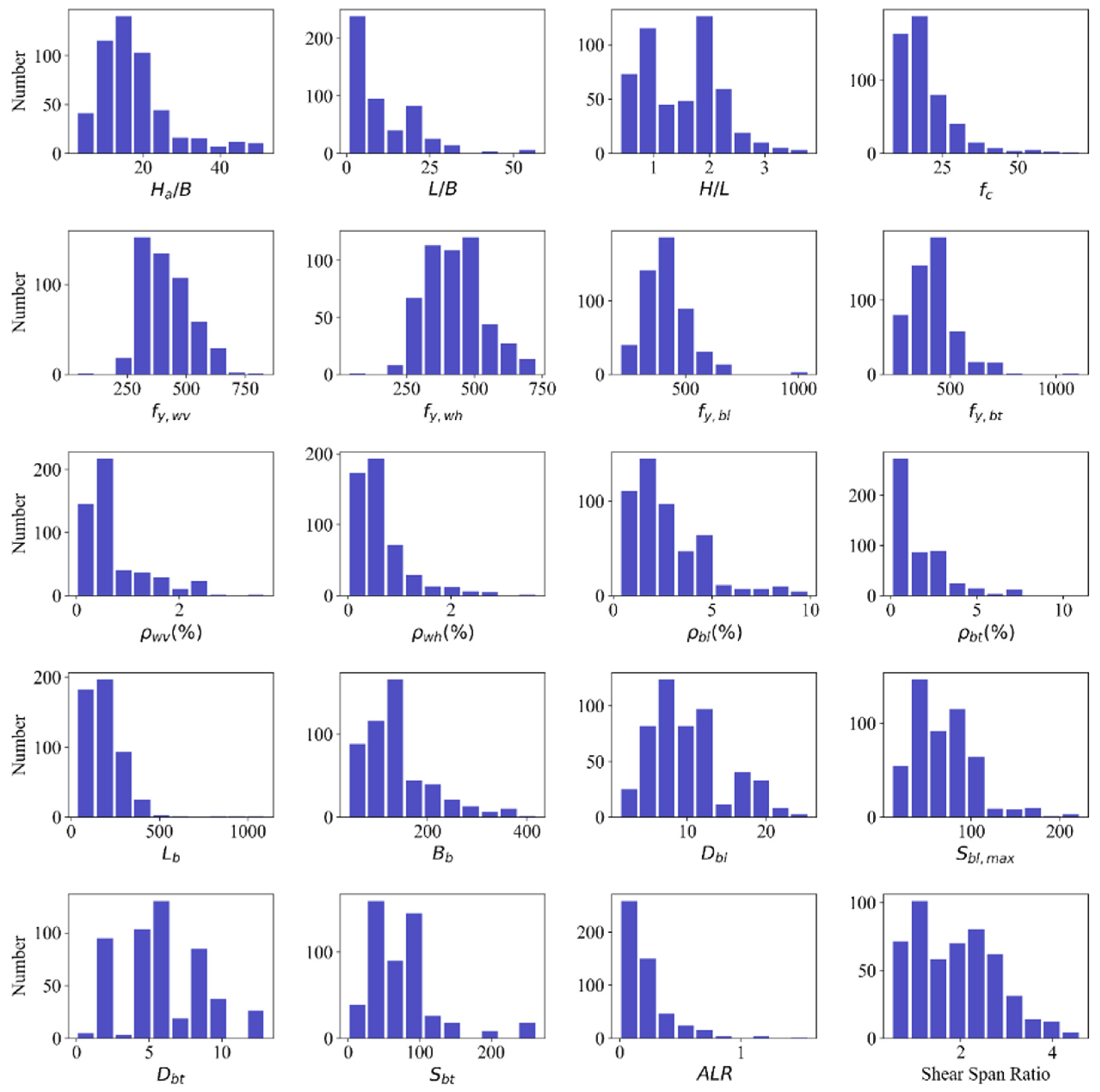
To fulfill the aims of this study, the samples with no boundary transverse reinforcement were cut out, and the database was filtered to include 503 wall specimens with BEs. The histograms of some parameters are shown in Figure 1. This includes 276 rectangular, 112 barbell, 70 flanged, and 24 T-shaped (web in compression) formations, as well as another 21 shapes. The meanings of variables are provided in Notation.

Figure 1.
The histograms of some parameters for 503 samples.
3. Method
This study is based on the ductility design method and ML methods. This study focuses on establishing a prediction model of boundary transverse reinforcement for RC shear walls with BEs, which is based on the ductility demand represented by the experimental drift ratio (). That is, our aim is to establish a model with a package of input variables including experimental drift ratio. Reasons for choosing the drift ratio instead of curvature ductility as the input ductility demand are given in other research [42] related to this study. There are three principal reasons for choosing the drift ratio as the input ductility demand: (1) the drift ratio includes bending deformation and shear deformation and is suitable for flexure-controlled, flexure-shear-controlled, and shear-controlled situations; (2) the drift ratio does not depend on the definition of yield displacement or yield curvature; (3) the drift ratio is a routine record of all specimens, and can be directly related to drift limits specified in building codes (T/CECS 392-2021 [43], ASCE 41-17 [44]). Frequently, the drift capacity of RC shear walls () is defined as drift corresponding to a 15% lateral strength loss from the peak strength in China. The target variable is a volumetric reinforcement ratio in the boundary elements, typically representing the volume of transverse reinforcement (like hoops or ties) in relation to the total volume of the confined core in columns or boundary elements.
A schematic overview of the methodology used to develop a prediction model of transverse reinforcement for RC shear walls with BEs in this study is shown in Figure 2. Key points of the prediction include the following: (1) data preprocessing, including the collection and classification of parameters, and their transformation for further study; (2) feature engineering, including dimensionality increases and reductions; (3) selection of an algorithm, involving the pre-training of eleven ML methods based on the training set, and performance evaluation of the testing set through three typical statistical metrics; (4) model training using the selected algorithm and optimization using hyperparameter tuning and cross-validation; (5) comparison with empirical equations and codes; and (6) interpretation of the results through the SHAP method and partial dependence plot (PDP). Following these steps, the selected model is compared with those proposed by researchers and codes to obtain a broad view and more informative details. Safety analysis is then implemented, with consideration paid to application in engineering practice. Finally, the model code is converted into C code for deployment in Chinese structural analysis software (SAUSAGE 2023) in order to conduct comprehensive structural analysis.
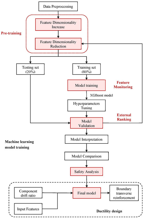
Figure 2.
Overview of procedure used to develop machine learning-driven boundary transverse reinforcement model based on the ductility demand.
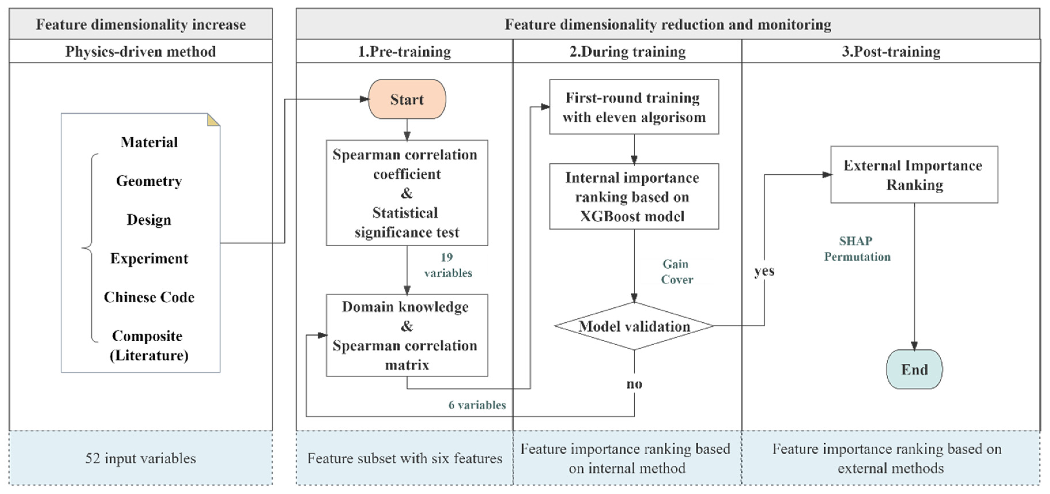
The fundamental objective of feature engineering is to identify a minimal subset of features that exhibit the highest degree of mutual orthogonality while capturing the most pivotal patterns intrinsic to the problem [18]. Feature dimensionality increase and reduction are two concepts commonly used in feature engineering [45]. Feature dimensionality increase is the process of exploring feature combinations, which involves data-driven methods with feature creation, the validation of physical quantities, and physics-driven methods with domain knowledge of the problem. Feature dimensionality reduction permeates three stages: pre-training, during training, and post-training. The basic workflow of the feature engineering utilized in this study is illustrated in Figure 3. This serves as a dynamic mechanism throughout the entire training process, primarily encompassing two aspects: feature dimensionality increases and reductions. Further, feature dimensionality reduction is categorized into three phases: pre-training, during training, and post-training.
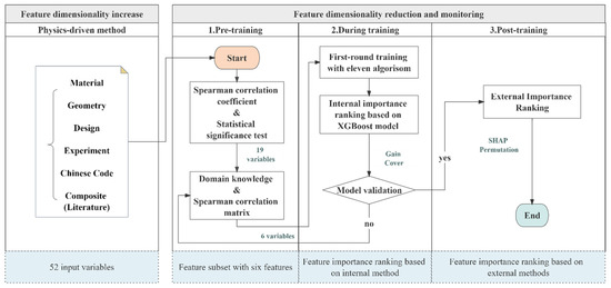
Figure 3.
The working line of feature engineering.
4. Machine Learning Boundary Transverse Reinforcement Prediction Model
4.1. Feature Dimensionality Increase
In this study, feature dimensionality increases are achieved via the physics-driven method, i.e., the collection of physical quantities that conform to fundamental laws. These are drawn from three sources: (1) simple variables from a database, such as height or thickness in geometry; (2) calculated variables used in design, such as axial compression ratio; and (3) composite variables utilized in previous research or codes. The input variables to be considered include materials, geometry, design, test to code-related, literature, and composite parameters. There is a total of 52 parameters, as shown in Table 1. It should be explained that the categorical variable, namely, the configuration of the boundary transverse reinforcement, is not set as an input variable. This is because most of the samples only have one identical single arrangement, with no evident difference between versions.

Table 1.
Initial selected features collected in the database.
Before the next step, preprocessing and transformation are implemented, because some of the categorical variables are not suitable for correlated analysis or certain algorithms. An encoding technique must be used to transform the categorical variables into numeric ones. In this study, target encoding (mean encoding) is adopted, where each category (loading modes and cross-sectional shapes) is replaced with the mean of the target variable for samples sharing that category.
4.2. Feature Dimensionality Reduction
Feature dimensionality reduction or feature selection is then performed to identify the most suitable feature subset for subsequent training by analyzing the relationship between input variables and the target variable. Statistical methods are utilized to obtain a subset with minimal features before model training.
Firstly, input variables weakly correlated with target variables are quantitatively assessed using the Spearman’s correlation coefficient, a non-parametric measure of rank correlation which assesses the strength and direction of association between two ranked variables. Unlike Pearson correlation coefficient, it does not assume that data are from a specific distribution. Hence, it can be used with ordinal, interval, and ratio data. Additionally, it assesses both linear and non-linear monotonic relationships. Thus, it is applicable to the data from this study. The coefficient is computed as:
where is the difference between the ranks of corresponding variables, and is the number of observations.
After analyzing the relationships in samples, validation should be further expanded to the population. Statistical significance testing provides mechanisms to determine if the result is likely due to chance or if there might be a genuine effect or difference, indicating whether the sample observation also applies to the population. Table 2 reports the Spearman’s correlation coefficient and the p-value from the statistical significance test. More details of the parameters are listed as Table A1 in Appendix A. A null hypothesis () is tested there, with a statement that there is no strong monotonic correlation in the population. The hypothesis test is expressed as and . The alpha level () is set at 0.05, meaning that a -value less than 0.05 indicates that the null hypothesis is invalid—that is, there is no strong association between the two variables. Overall, 33 input variables with or are typically eliminated.
Table 2.
Spearman’s correlation coefficient and -value between each feature and transverse reinforcement in filtered variables.
Secondly, with the aim of establishing a minimal subset of features that exhibit the highest degree of mutual orthogonality, there is a need to reduce variables for model training by cutting off the highly correlated variables in the preselected subset above. Through domain knowledge and the Spearman correlation matrix, groups of input variables with high mutual correlation are identified. Only one feature is retained for each pair and used to mitigate their potential influence on the model outcomes. Obviously, , , and display direct computed relationships with the target variable () and ductility demand (). is included in the parameter with higher value. Similarly, and are also parts of parameters with higher value, namely and . Thus, , , , , , and are removed before proceeding to the next phase. It can also be seen in Table 2 that the ductility demand as an indicator of the prediction in this study, is very suitable because of its relatively high ranking and low -value compared with the ductility factor ().
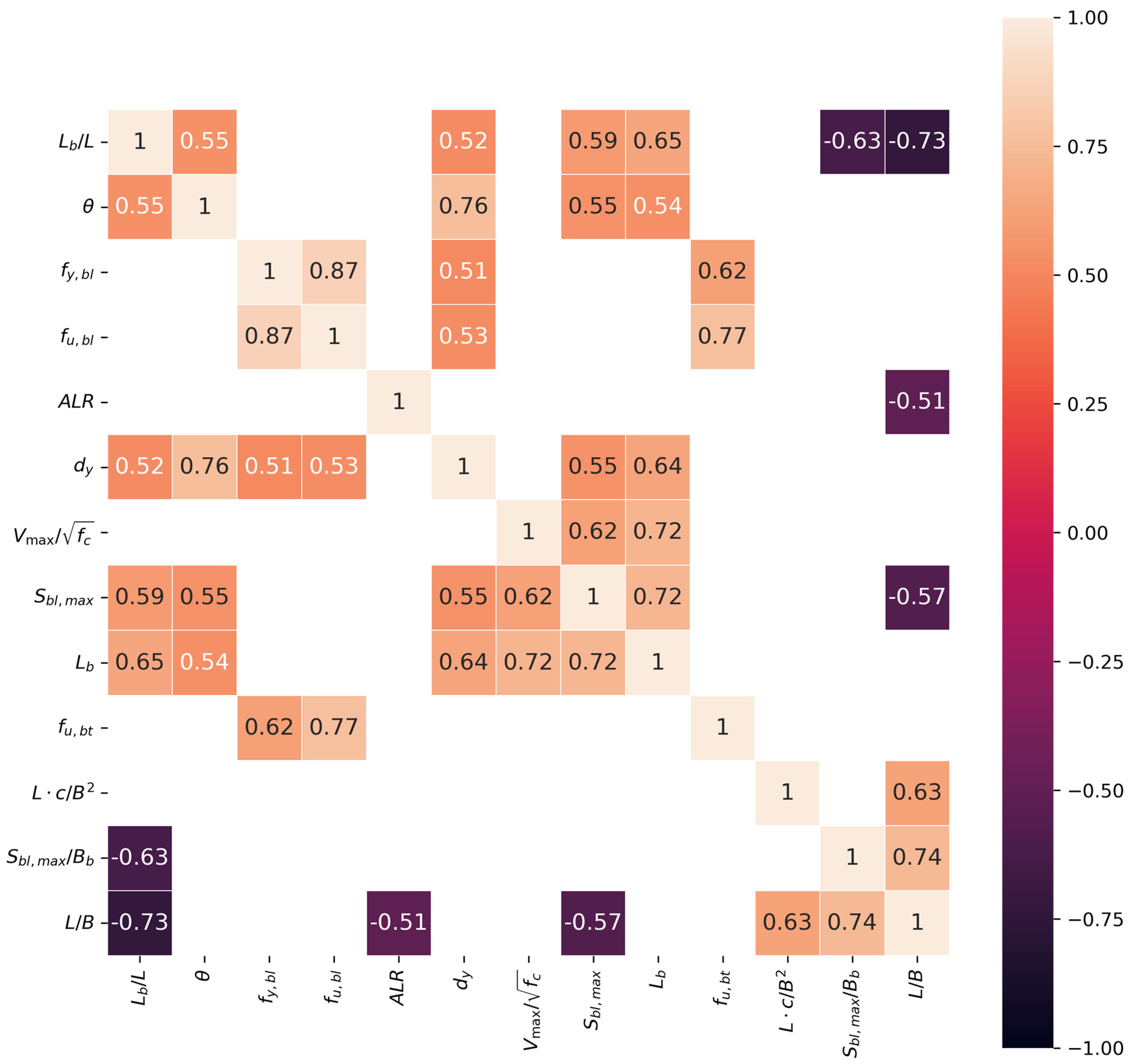
In general, it is good practice to remove highly correlated features prior to training, regardless of the adopted algorithm. Thus, only several features are retained for each pair of highly correlated features. Figure 4 presents the Spearman correlation matrix, in which there are three pairs of highly correlated features (): (1) —, , , ; (2) —, ; (3) , , —. To fulfill the aim of this study, four input variables relevant to the factor () in this study are removed. In the second pair, displays stronger correlation with transverse reinforcement and a lower -value compared with its correlated versions, meaning that it is retained in the second group. is simultaneously related to other input variables within the same group, which indirectly indicates that it can be largely characterized by the other variables. In order to maintain both the relative completeness and diversity of information conveyance, it is excluded here.
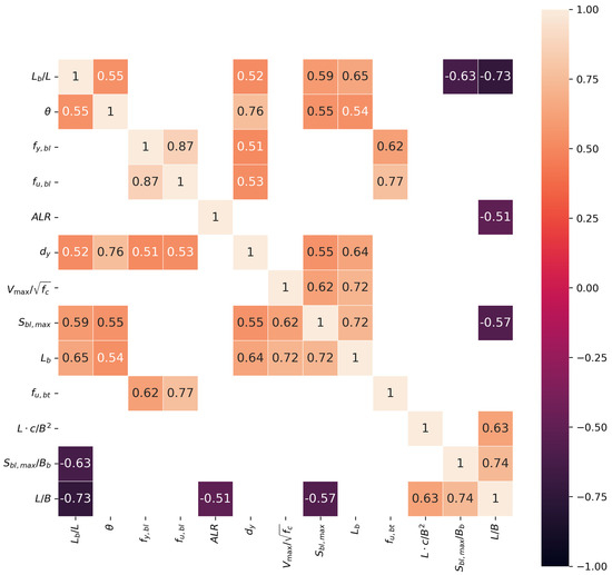
Figure 4.
Spearman correlation matrix with .
In summary, a robust feature subset can be defined as one that encompasses the maximum amount of effective information with the smallest subset size, while also minimizing mutual interference among features. This subset is selected from input variables via the following process:
- (1)
- Weak correlation elimination with the target is conducted by utilizing Spearman’s rank correlation coefficient () to compute and explore nonlinear relationships between input variables and the target variable. Validating the applicability of these patterns from the sample to the general population via significance testing () identifies nineteen input variables with strong correlation to the target variable;
- (2)
- Physical dimensionality reduction is performed. Leveraging domain knowledge in civil engineering, the nineteen input variables are subjected to substitutability analysis, eliminating replaceable variables;
- (3)
- Elimination of collinear input variables is conducted, using the Spearman correlation matrix to identify groups of variables with strong correlations. The selective elimination of highly correlated input variables within each group ensures that the feature subset conveys more effective information within a simplified structure, reducing the mutual influence of input variables. This approach enhances the precision of model training and reduces subsequent computational demands.
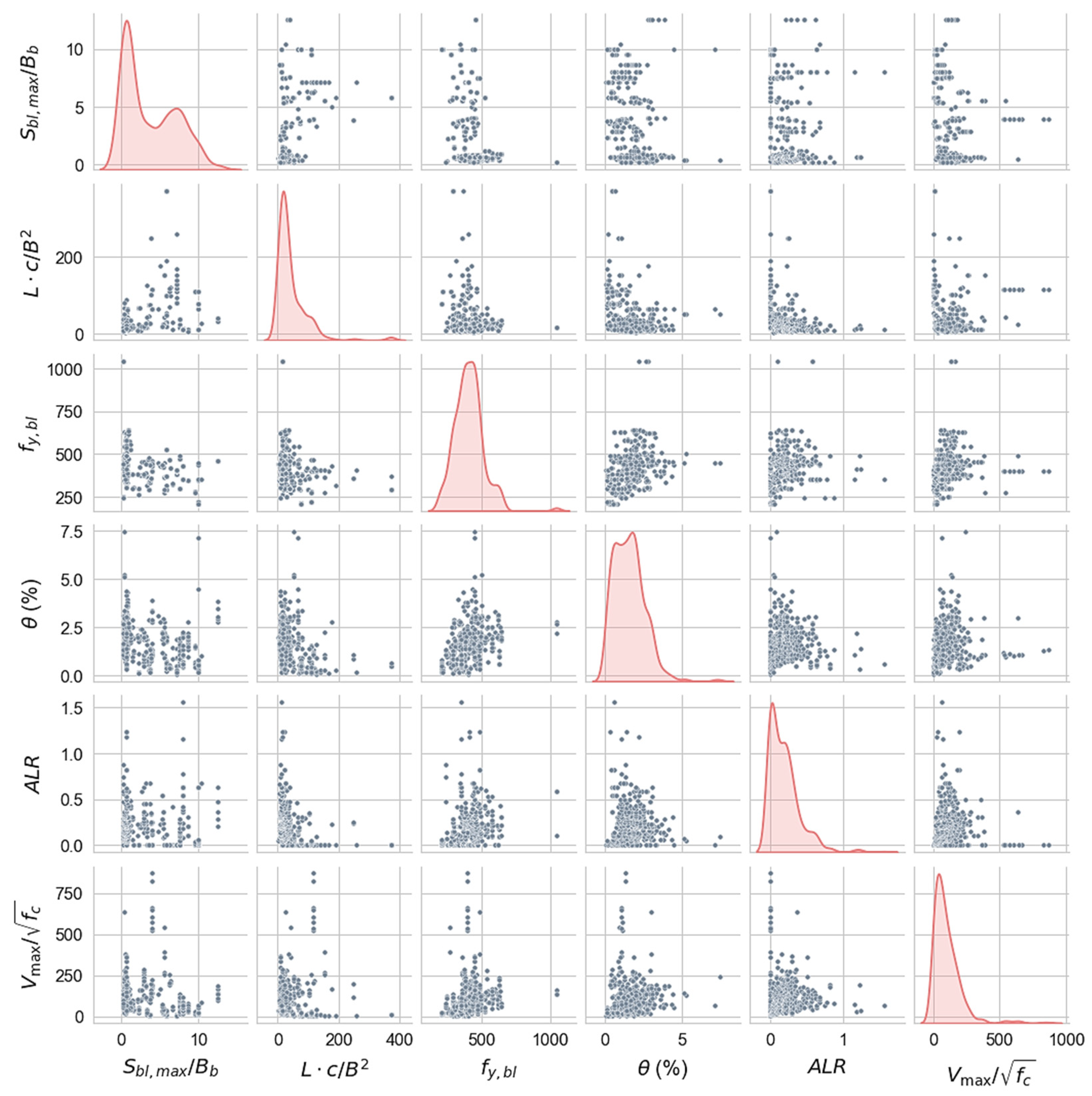
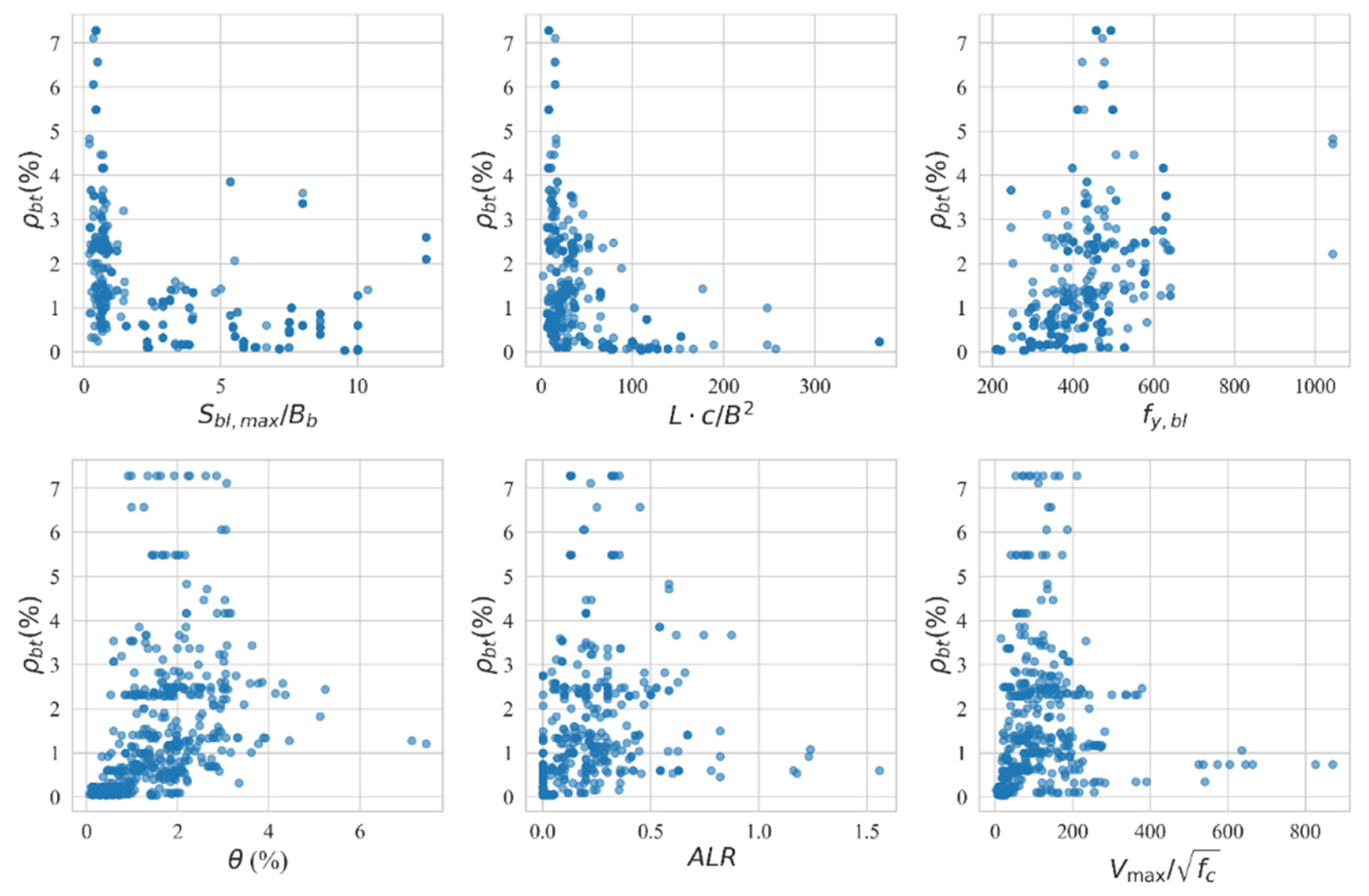
Finally, six input variables, namely, , , , , , and , are selected through the following steps and they constitute the feature subset for model training. The scatter matrix is shown in Figure 5, and the variation in transverse reinforcement with respect to each feature is given in Figure 6. These values, respectively, represent the yield strength of the longitudinal reinforcement in BEs, the ductility demand, the level of shear stress related to the failure mode, the ratio of the spacing of longitudinal reinforcements along the length of the wall to the thickness of BEs, the relative slenderness of BEs, and the design axial load ratio. Each of these factors is physically related to wall deformation. In other words, they are all potentially associated with the configuration of boundary transverse reinforcement.
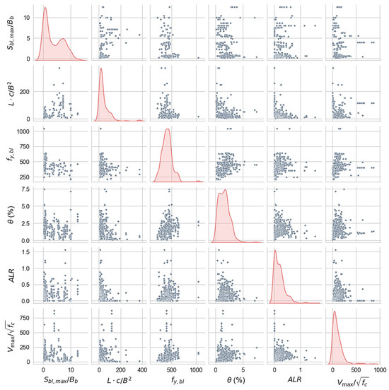
Figure 5.
Scatter matrix and kernel density estimation (KDE) plot of six features.
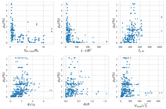
Figure 6.
Variation of transverse reinforcement with respect to each feature.
4.3. Statistical Metrics for Model Performance
The evaluation of performance in prediction models utilizes statistical metrics, which take into account both the predicted and observed transverse reinforcement. In this study, metrics should be suitable for use in regression problems of continuous targeted values. When the evaluation of different algorithms is compared in order to choose the most applicable method, a combination of metrics is applied. The first metric is the coefficient of determination () (Wright, 1921) [46], which can be interpreted as the proportion of the variance in the dependent variable that is predictable from the independent variables, ranging from to 1. This parameter is deployed to detect the quality of the performance of a regression method, and is among the more informative and truthful. Additionally, it does not display the interpretability limitations of other metrics [47]. The second metric, the weighted absolute percentage error (WAPE), is the weighted average of the ratio of the absolute value of the difference between the actual and predicted values to the sum of the actual values. It is a summary statistic that provides a holistic global error assessment, focusing on the overall degree of prediction error. The third metric, the root mean square error (RMSE), indicates the square root of the mean of the squared differences between the predicted and actual values. This value can efficiently reflect significant differences, because it is sensitive to outliers and penalizes large errors more severely.
4.4. Machine Learning Algorithm
A feature subset of six features is utilized to pre-train the model. Some 11 algorithms are considered and compared to select a suitable one. The first group comprised (1) linear algorithms: ordinary least squares (OLS), lasso regression (lasso), ridge regression (ridge), K-nearest neighbors (KNN), and support vector regression (SVR). We also considered (2) tree-based algorithms: decision trees (DT), random forests (RF), AdaBoost, LightGBM, and CatBoost, as shown in Table 3. Among the tree-based algorithms, there are two categories of strategy, namely, parallel ensemble techniques (bagging methods) and sequential ensemble techniques (boosting methods). Linear regression models are utilized as the basic model for comparison. Comparing the predictions of several linear models, tree-based models increase accuracy and dig out potential nonlinear relationships.
Table 3.
Comparing performance of XGBoost model.
In pre-training process, the training set (80% of the data) is utilized to train the models based on 11 algorithms. Then, the performance is evaluated based on the testing set by comparing the predicted values with the experimental data, as shown in Table 3. Tree-based models display better performance than linear models. Statistically, a model with a high value of and corresponding low values of error (RMSE, WAPE) is considered to possess better performance in terms of accuracy and robustness (the three metrics are summarized in Section 4.3). The XGBoost algorithm [48,49] is selected as the final prediction model of boundary transverse reinforcement via comparison with various algorithms, because it shows the best performance ( = 0.819, RMSE = 0.239, and WAPE = 0.294) on testing sets among all 11 ML models.
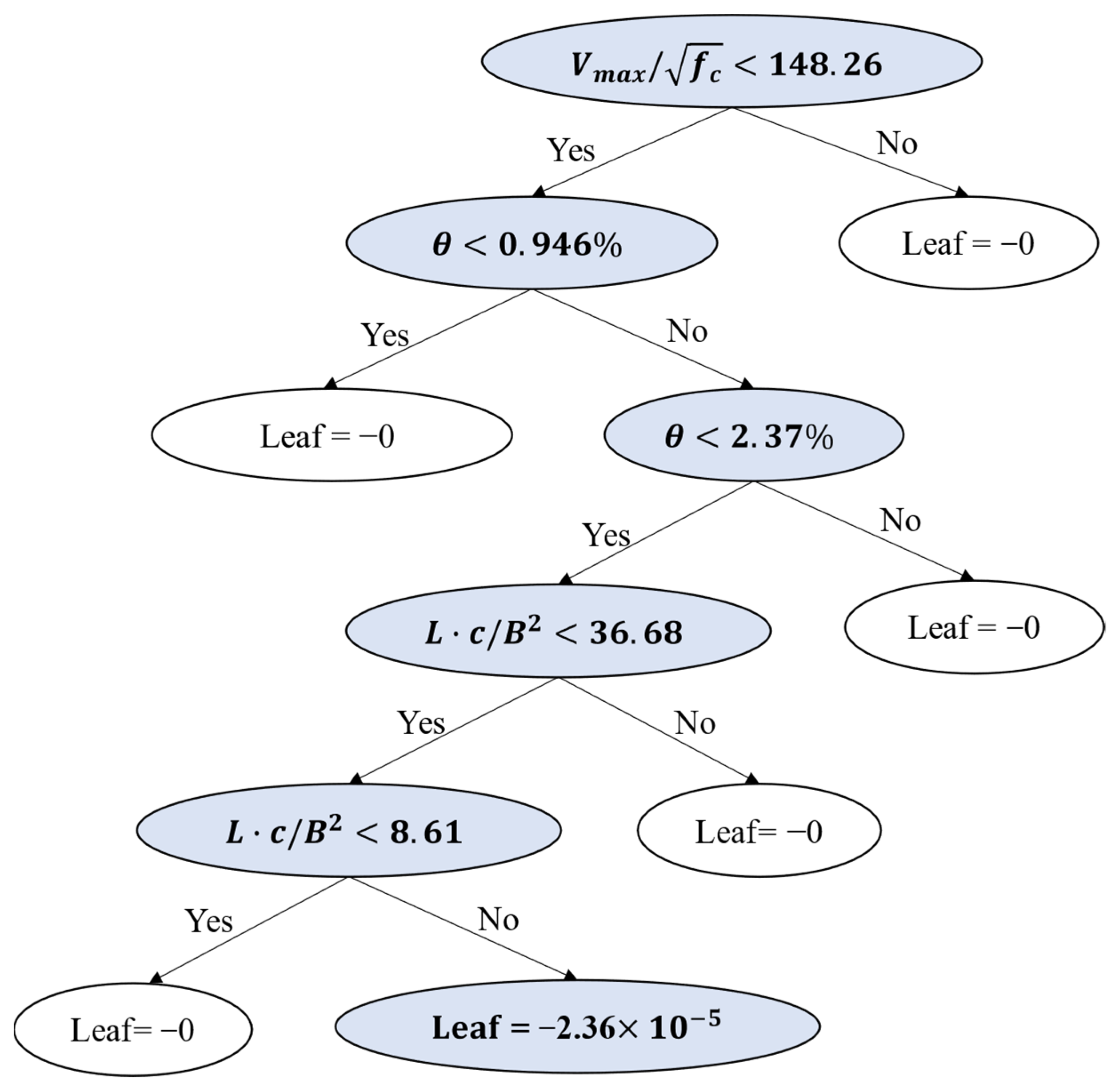
Additionally, we remove two samples after pre-training because of the outlier degree, which exerts a negative effect on accuracy. An example of the final XGBoost model weight tree for this study is shown in Figure 7.
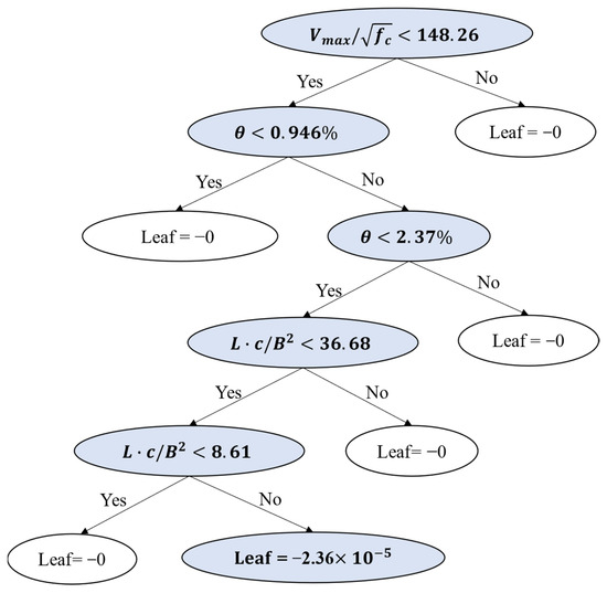
Figure 7.
XGBoost model weight tree.
4.5. Model Training with Hyperparameter Tuning and Cross-Validation
After selecting the model training algorithm, it is necessary to adopt reasonable methods for training and prediction and to optimize the selection of hyperparameters. It effectively enhances the generalization ability while reducing the likelihood of overfitting during the training process. This involves hyperparameter selection and model training methods. In this study, k-fold cross-validation (CV), ratio sampling, and grid searching are combined to train the final model with the optimal combination of model parameters.
This study uses the following methods to optimize the model. We apply a random split with 20% data for testing and 10-fold cross-validation to process a single round of training and prediction, whereby single rounds are repeated 100 times via random ratio sampling. To obtain the best output from the final model, grid search is applied to tune hyperparameters. Eight hyperparameters are considered for tuning, and they are listed in Table 4. We built and evaluated every combination of these factors. The combination with relatively higher value of and lower values in RMSE and WAPE is selected. To alleviate the inherent randomness of selecting training and testing samples, a k-fold cross-validation process is employed [42]. Finally, under conditions of very small error variability, the overall performance is improved. The of the original model increases from 0.819 to 0.884, marking an improvement of 8%. The statistical performance of the final XGBoost model is listed in Table 5. Additionally, as a variant of the coefficient of determination, the adjusted R-squared value considers the influence of the number of features on the complexity of the model and is used to perform feature selection or reduction during training.
Table 4.
Hyperparameters adopted in XGBoost model of this study.
Table 5.
Statistical performance of XGBoost model.
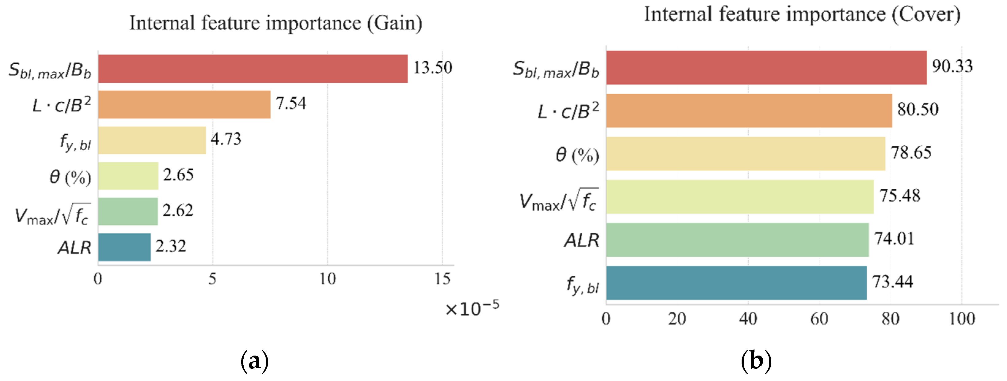
While training, a model-based or internal method is seen as a means of performing feature selection, providing direct assessment of the importance of features according to the current model, and offering instruction for feature adjustments. The gain (Gini importance) and cover of the XGBoost model offer a more holistic view of the feature’s contribution. Gain (Gini importance) refers to the average optimization of information gain (objective function) brought by the feature corresponds to the reduction in prediction error after the feature is split during node splitting. The higher the value of this feature, the greater its contribution to enhancing the performance of the model. Cover refers to the number of samples covered by the leaf nodes of a feature divided by the number of times the feature is used for splitting in tree models during splitting. The closer the split is to the root, the larger the cover value, indicating that the feature covers a larger scale of node splits in the model. This can be used to complement and verify the ranking results of Gain. Determined based on distinct objectives, external importance analysis is employed to comprehensively discern the influence of individual features within the model on the final outcomes with greater confidence in the results. In this study, two ways of ranking external importance are given to reflect the points of different emphasized in later sections, namely, the SHAP method and the permutation importance method.
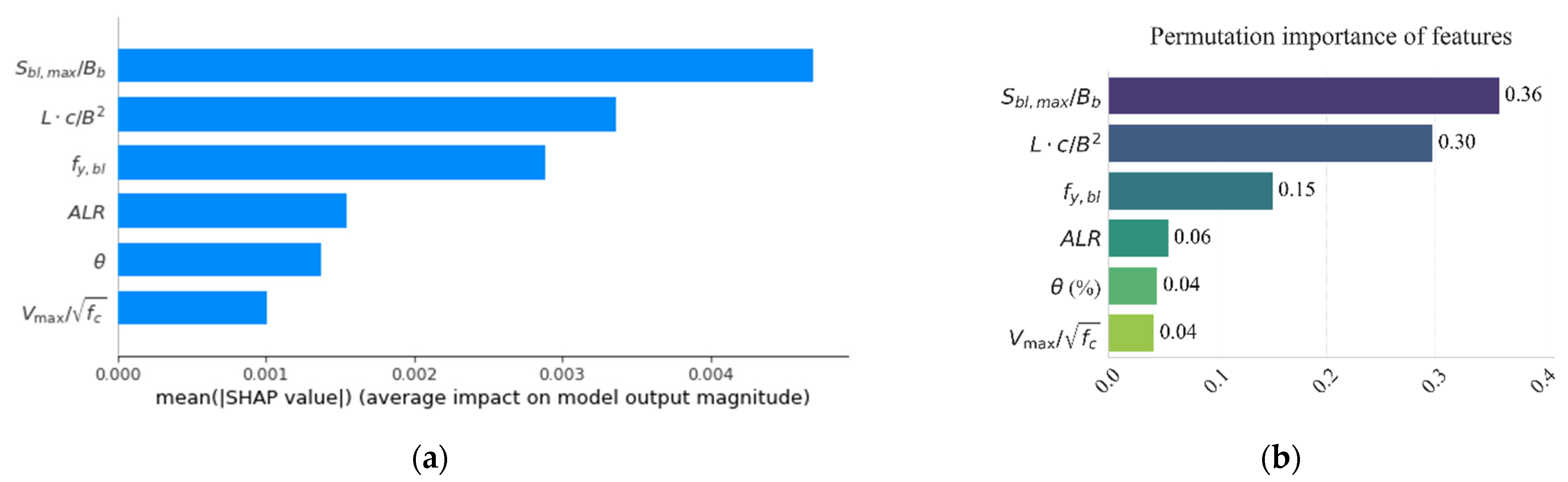
Internal importance rankings of features are obtained, as shown in Figure 8. The greater enhancement of a feature means that it makes a more important contribution to the performance improvement of the model, where gain refers to the reduction in prediction error due to segmentation using this feature. Additionally, external methods are applied to provide more perspectives of relationship between features and the model, as shown in Figure 9. Permutation importance reflects the degree of depreciation of the target after the corresponding feature is scattered, while the SHAP value shows the marginal effect of the feature being removed. , , and display the highest feature importance values on most occasions. In both internal and external methods, and emerge as the predominant features. Their significance suggests that they play a crucial role in enhancing model performance, including in the presence of disturbances. and score higher in internal ranking (cover), but behave relatively worse in external ranking, showing that the disturbance to the model is weaker when each of these two features changes. The performance of the model is more sensitive to changes in and as they have higher scores in external ranking.
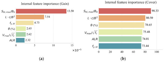
Figure 8.
Feature importance of XGBoost model based on internal ranking: (a) gain; and (b) cover.
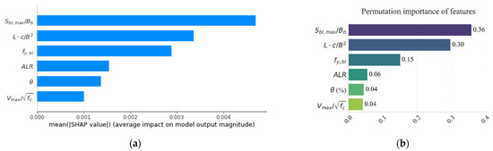
Figure 9.
Feature importance of XGBoost model based on external methods: (a) SHAP method; and (b) permutation importance method.
4.6. Interpretation of XGBoost Transverse Reinforcement Model
To understand the behavior of the proposed XGBoost model, tools for global explanation, local explanation, and error analysis are used to obtain greater understanding and interpretation. On the basis of robust statistical indicators and small errors, the trend of the feature’s impact is explained by SHAP values and a partial dependence plot (PDP).
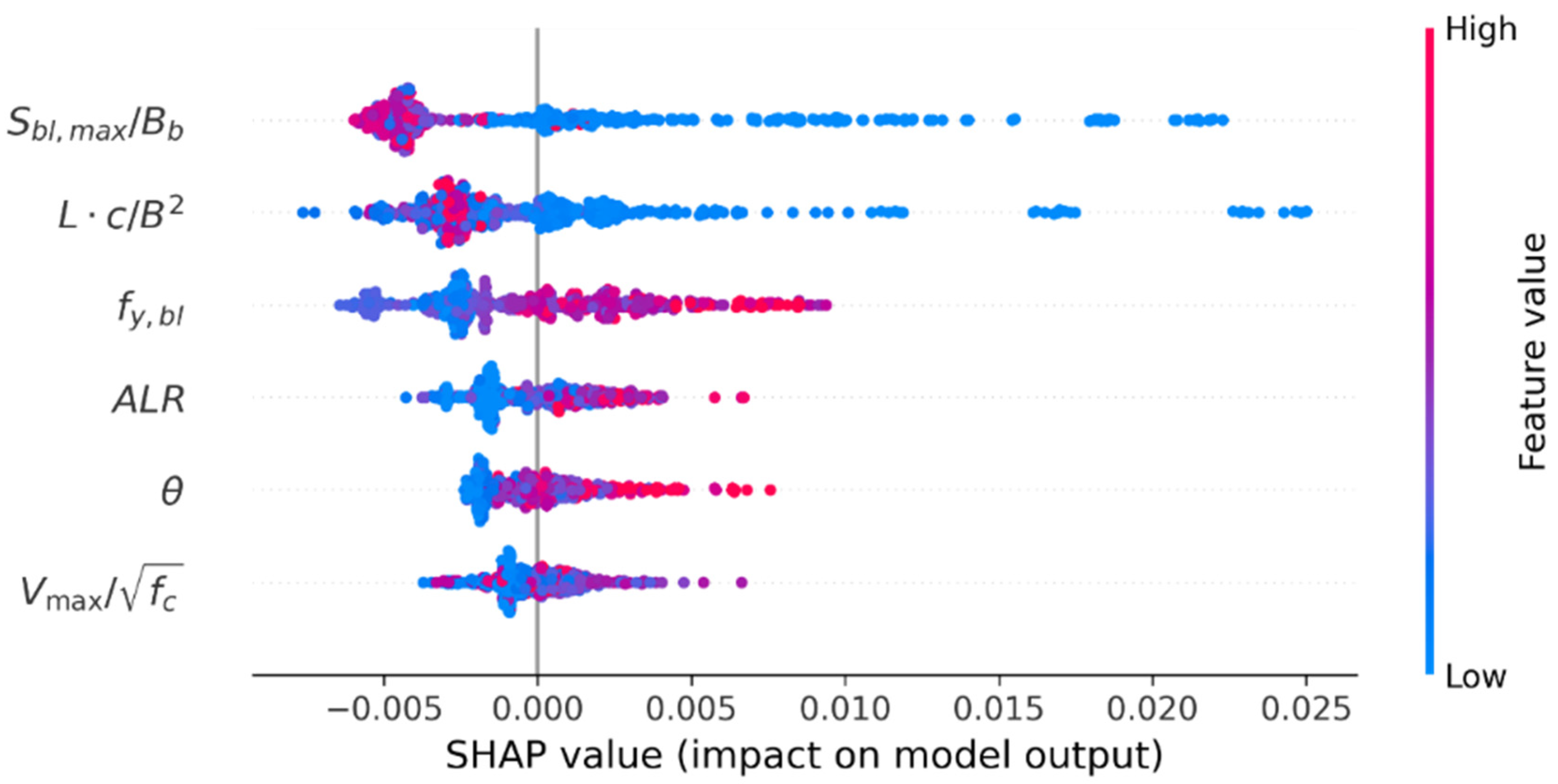
SHAP values, proposed by Lundberg and Lee [50], are computed to obtain a global explanation of the prediction trend affected by features. Figure 10 presents the SHAP summary plot for an XGBoost model trained on 501 samples. It illustrates the impact of each feature on the output, as conveyed by SHAP values derived from the XGBoost model. The horizontal axis, representing the SHAP values, reveals their influence on the predicted variable. Features are placed in order on the vertical axis based on their SHAP importance. SHAP values closer to zero suggest a less significant impact on the prediction, while values further from zero imply a more pronounced influence. The dots symbolize samples from the database. Their color, transitioning from blue to red, indicates the progression of feature values from low to high. The dot density represents the concentration region of a particular feature. When interpreting the impact trend of individual features, (1) the progression of the corresponding row from left to right and the distinct change in the dot color from blue to red indicates that an increase in the feature value is favorable for enhancing transverse reinforcement. The trend is the opposite when the change is from red to blue. (2) The broader the range provided by the SHAP values and the sparser the dots, the more sensitive the predicted variable is to alterations in feature values. Furthermore, (3) in areas where dots are predominantly clustered in blue and located on the left of the zero axis, it is possible to surmise that that for most classifications with small feature values, a smaller value of this feature is unfavorable for transverse reinforcement. The interpretations for other scenarios are analogous.
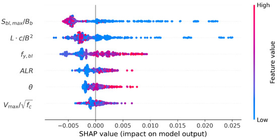
Figure 10.
Impact of features for transverse reinforcement on XGBoost model.
In this model, exhibits the greatest predictive power, followed by and then . It should also be observed that high and values are associated with lower boundary transverse reinforcement. For and , the opposite conclusions are drawn. This aligns with a multitude of experimental findings suggesting that boundary longitudinal reinforcement with a higher yield strength, greater ductility demand, and larger design axial load ratio increases the transverse reinforcement in the boundary element. The influence trend for is not evident. Simultaneously, both and exhibit a broader SHAP value range, and smaller values display a more pronounced impact. This suggests that the prediction of transverse reinforcement is sensitive to the abovementioned features, rendering them unsuitable for referencing in boundary transverse reinforcement design, even if they possess greater importance. In contrast, the ductility demand () used in this study displays a narrow SHAP value range. As the value increases, the SHAP value changes uniformly, and the negative impact is minimal, causing less perturbation to the model. The concentrated values for both and are for larger feature values, whereas the other four features are for smaller values.
Additionally, a partial dependence plot (PDP) [49,51,52] is a visualization tool that displays the marginal effect of one or two features on the average prediction of a machine learning model. PDP plots are typically represented graphically, where the x-axis represents the values of the feature and the y-axis represents the predicted value of the model. Each light-colored line represents the result line of one sample. For easier viewing, only 100 individual sample result lines are displayed, while the dark-colored line is the average line of all samples. It can help to understand how the model predictions change when the feature values increase or decrease. Figure 11 displays the one-way PDPs of predicted boundary transverse reinforcement with different features in the XGBoost model. The trends that correspond to different features are essentially consistent with the patterns presented in the SHAP plot. This provides a reliable basis for the identified patterns and visually demonstrates the degree of change in prediction for different value segments. Among these trends, both and exhibit a distinct negative relationship with the prediction, especially within the intervals , and . exhibits a clear positive relationship with the prediction, although a negative relationship is evident in the range . The relationship between the change in and the predicted transverse reinforcement is complex. Overall, it is a positive relationship, especially in the intervals and . However, when the axial load ratio increases (i.e., ), a negative relationship is instead revealed. The impact of on the prediction is not pronounced (it is positively correlated when , and essentially unchanged when ). displays a clear positive relationship with the prediction (it is positively correlated when and , and negatively correlated when ). It is worth noting that, with the changes in , , and , the average predicted value range is between 1% and 2.5%. With the fluctuations in , , and , the predicted value primarily hovers between 1% and 2%.
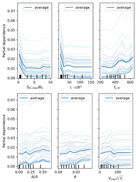
Figure 11.
One-way partial dependence plots of features.
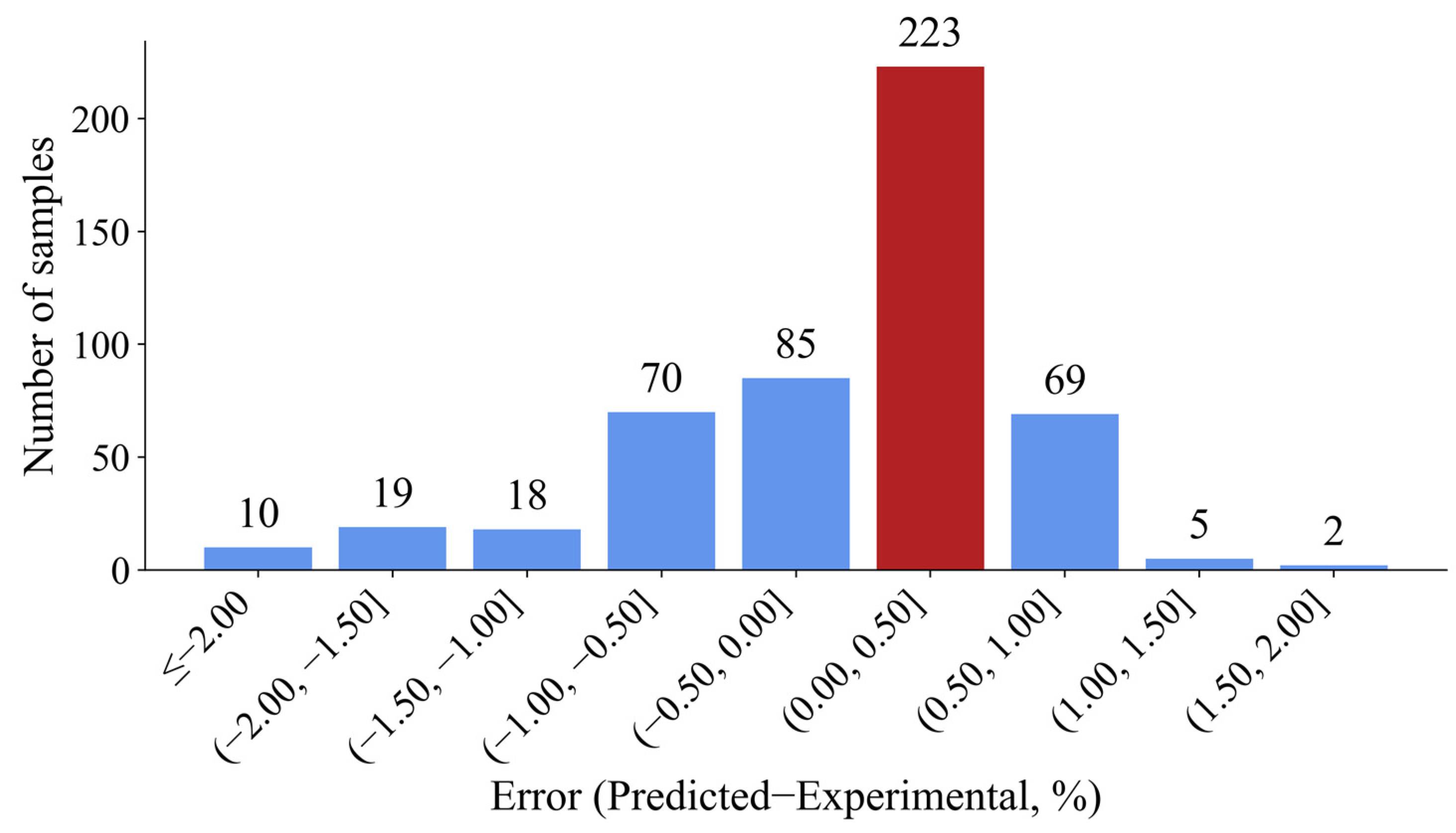
In addition, residual analysis is also used to reflect the specific errors in the trained model based on the selected algorithm. A variant of the coefficient of determination, known as adjusted R-squared, considers the influence of the number of features on the complexity of the model, and is used to feature selection or reduction during training. A histogram of errors for the XGBoost model is shown in Figure 12. As illustrated in Figure 12, there are more samples with positive error (predicted value greater than the experimental value, approximately 3/5). Approximately 90 percent of the sample error is within 1% of the absolute value, including the interval with the largest error between 0 and 0.5%.
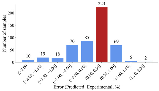
Figure 12.
Histogram of errors for the XGBoost model.
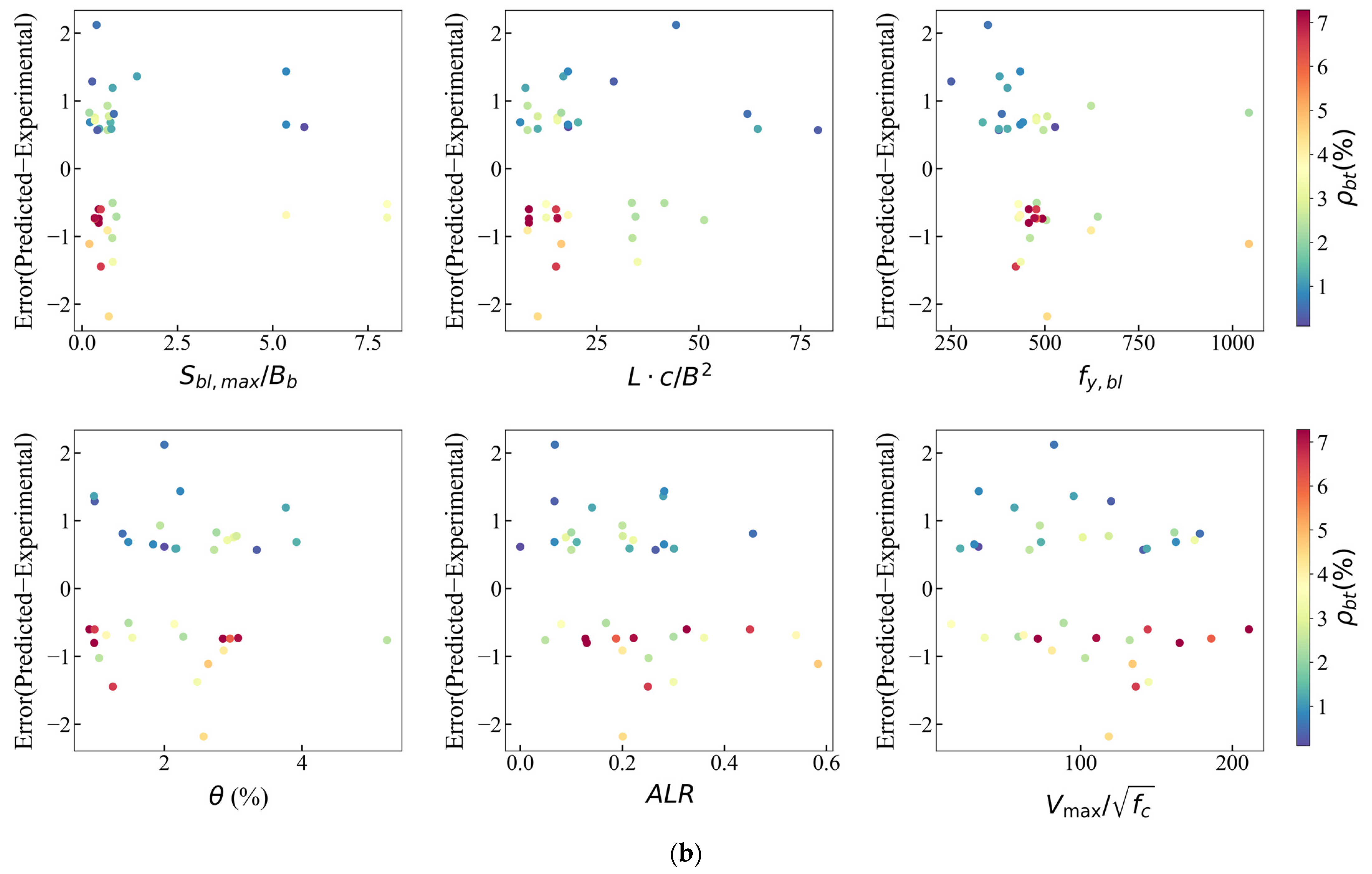
In order to further investigate the relationship between the error distribution and features and quantify the scope of application of each feature in the model with relatively lower error, error scatter plots are plotted, as shown in Figure 13. Figure 13a displays the error points for samples with smaller or larger experimental boundary transverse reinforcement, and they tend to be symmetrical. After further investigation of the data points with the highest (>0.5%) absolute error values, Figure 13b is displayed. It is observed that most of the higher errors appear to be concentrated in the lower values of , , (), and . The error distribution has no obvious trend with the change in .
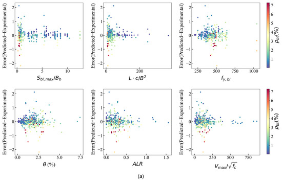
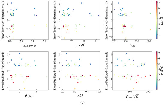
Figure 13.
Variation of error for XGBoost model: (a) all samples; (b) error.
4.7. Comparison of Empirical Equations and Codes
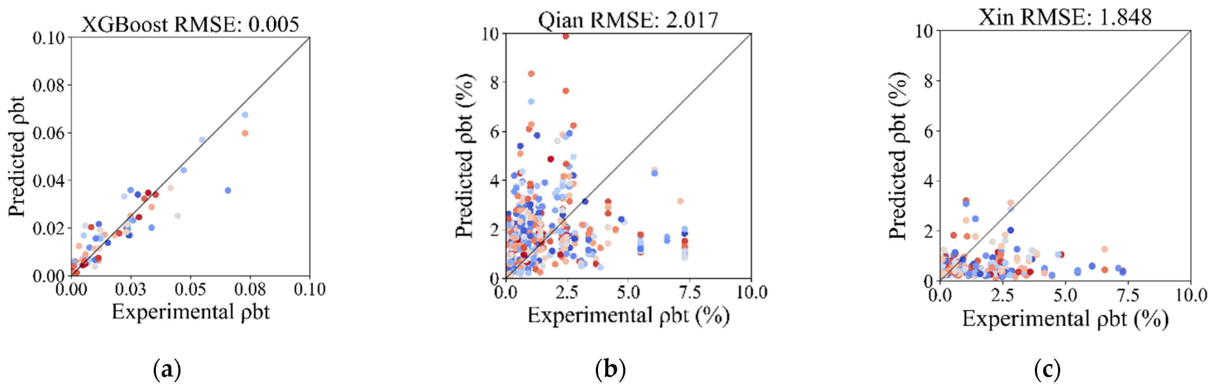
In order to validate the applicability and potential superiority of the proposed XGBoost model, traditional empirical models proposed by researchers and codes are used to predict the transverse reinforcement ratio and test the performance with the same data utilized in this study. GB1–3 correspond to three different combinations of seismic degrees and seismic precautionary intensity in the Chinese code [10], indicating decreasing severity. Methods in the US code (ACI 318-19) [11] and the European code (Eurocode 8) [12] are also included. The results are displayed in Figure 14 and listed in Table 6.
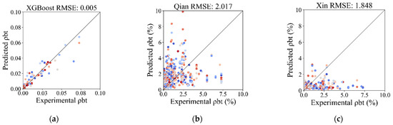
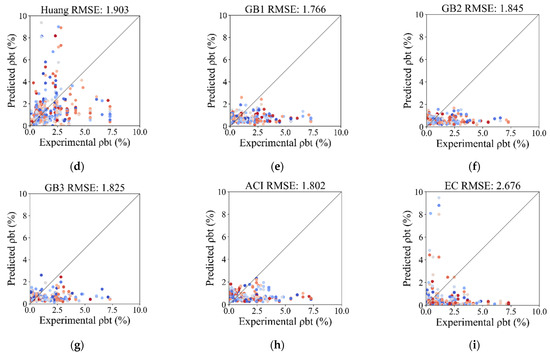
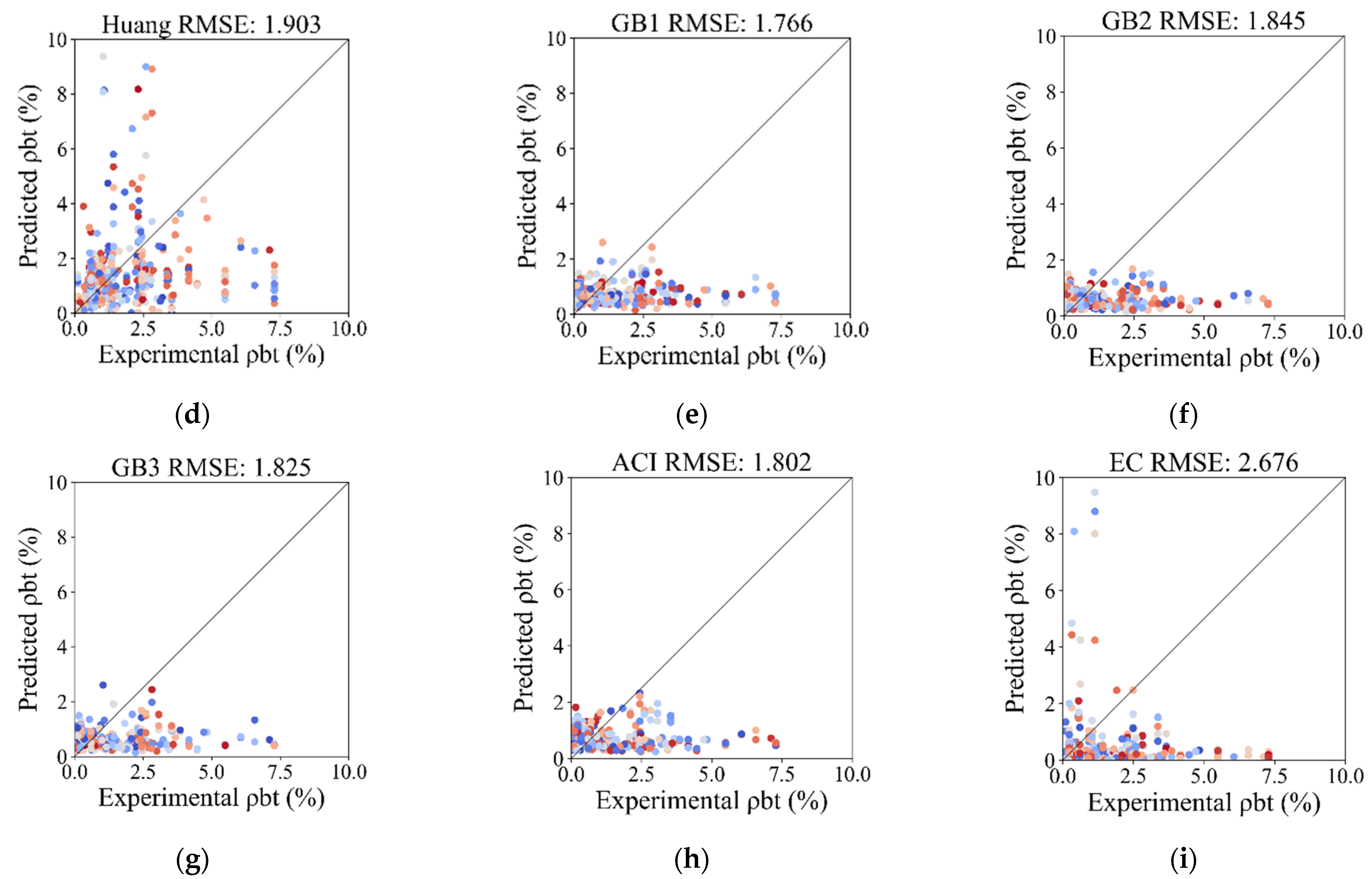
Figure 14.
Comparison of predicted and experimental transverse reinforcement ratio with empirical models: (a) XGBoost model; (b) Qian et al. [7]; (c) Ma et al. [8]; (d) Huang et al. [9]; (e) GB1; (f) GB2; (g) GB3; (h) ACI 318-19; (i) EC (2006).
Table 6.
Comparing performance among XGBoost model and empirical models in studies and codes.
Figure 14 and Table 6 show that the predictive performance of the proposed ML model is more accurate, robust, and stable than that exhibited by its competitors. In Figure 14, the root mean square errors (RMSEs) of the empirical formulas of Qian et al. [7], Ma et al. [8], and Huang et al. [9] are 2.017, 1.848, and 1.903, respectively, while the RMSE of the XGBoost model on the testing set is 0.005. The standard deviation values of the error between the experimental and predicted transverse reinforcement ratios of the empirical formulas of Qian et al. [7], Ma et al. [8], and Huang et al. [9] are 1.997, 1.620, and 1.881, respectively, while that of the XGBoost model on the testing set is 0.005. The figures show greater sensitivity and lesser accuracy in empirical formulas than those produced using the XGBoost model. This also reflects the robustness and stability of the ML model in prediction compared with empirical methods, because RMSE is sensitive to outliers and penalizes large errors more severely. In Table 6, the lowest weighted absolute percentage error (WAPE) of three types in the Chinese code (GB 50010-2015) [10], ACI 318-19 [11], and Eurocode 8 [12] is 0.772, which is obviously higher than that of the XGBoost model, with a value of 0.246. This shows that the overall predictive performance of the XGBoost model is better, because WAPE is a summary statistic that provides a holistic, global error assessment which focuses on the overall degree of prediction error.
The primary reasons for and advantages of the superiority of the XGBoost model can be attributed to the following facts: (1) Empirical formulas are derived based on a limited number of original shear wall specimens, which implies that the accuracy and applicability might be constrained by the scope (e.g., cross-sectional shape and level of confinement) and diversity of the initial experimental data (e.g., axial load ratio). They may not be fully applicable to new situations or a broader range of shear wall types that significantly differ from the original data. However, this could be improved in XGBoost models based on the richness of the newly built database. (2) The ability of ML methods, especially tree-based algorithms, to dig out complex and nonlinear relationships is stronger than that of traditional linear regression formulas. (3) Empirical formulas might neglect, overestimate, or underestimate parameters that contribute to the transverse reinforcement ratio, due to the restriction of computing and analysis abilities.
Qian et al. [7] model:
Ma et al. [8] model:
Hang et al. [9] model:
4.8. Safety Analysis
Figure 15 displays the histogram and empirical cumulative distribution of the error between the experimental and predicted transverse reinforcement ratio of the XGBoost model when applied to testing sets. The vertical line at error = 0 indicates that the predicted value is equal to the experimental value. Errors less than 0 indicate safety, whereas errors larger than 0 indicate insecurity. Most of the transverse reinforcement ratios predicted by the XGBoost model are very close to the experimental values, with a safety probability of 57%.
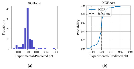
Figure 15.
Distribution of the error between experimental and predicted transverse reinforcement ratio on testing set: (a) histogram; (b) cumulative distribution function.
When applied in engineering practice, factoring in safety, structural stability, and reliability, the prediction model should be sufficiently conservative to ensure the safe design of RC structures. Acceptance criteria (AC) [50] provide limiting values of properties, such as drift, strength demand, and inelastic deformation. These are used to determine the acceptability of a component at a given performance level. ASCE 41-17 [44] provides a procedure for defining AC based on experimental data. However, for more severe performance objectives related to safety and structural stability, considerations for the selection of AC should reflect the probability of exceeding a threshold behavioral state (i.e., life safety, LS, and collapse prevention, CP) [41,53], corresponding to the onset of lateral-strength degradation or axial failure. This method is more appropriate and consistent with the performance objectives of columns in ACI 369-17 [54] by Ghannoum and Matamoros [53].
As primary components, shear walls must resist seismic forces and accommodate deformations if they are to achieve the selected performance level. Additionally, acceptance criteria with a fixed probability are recommended by Wallace and Abdullah [41]. When assessing a member critical to the stability of a structure, its ability to satisfy the AC for LS would indicate an 80% level of confidence that the member under consideration has not initiated lateral strength degradation [41]. On this basis, an additional value of 0.24% should be added to the value predicted by the XGBoost model established in this study. Furthermore, in order to meet different demands, several additional values with guaranteed rates are provided in Table 7.
Table 7.
Guarantee rate and related additional value of transverse reinforcement ratio.
5. Summary and Conclusions
This paper presented a machine learning (ML)-driven transverse reinforcement prediction model for application to reinforced concrete (RC) shear walls with boundary elements (BEs) based on the ductility demand. Using 501 shear wall samples, our research provided a valuable quantitative reference for both new and existing buildings.
- A new database of 291 shear wall samples was established with more detailed sample information and label categorization, offering available data and references for related research;
- A stable XGBoost model with = 0.884 was developed based on the feature subset (, , , , , ). This technique provides superiority in prediction, with higher accuracy, robustness, and lower variability than empirical formulas and standards;
- The developed model underwent feature monitoring and comprehensive analysis via the internal feature ranking (gain and cover) of XGBoost algorithms and by being subjected to external feature ranking methods (SHAP method and permutation importance). Both during and after training, the results indicate that the most influential factors on predictions are and . Simultaneously, and exhibit a negative relationship with boundary transverse reinforcement, while , , and show a positive relationship. This is in accordance with empirical findings, validating the reliability of the established model. The impact of is less pronounced in this model;
- Safety validation was conducted before application to ensure its practical value. Additionally, the source code of the model was converted into C code for deployment in structural analysis software to facilitate real-world engineering verification.
Author Contributions
Conceptualization, J.D. and C.X.; Methodology, J.D., J.L., C.X. and B.Q.; Software, J.D. and B.Q.; Validation, J.D.; Formal analysis, J.D.; Investigation, J.D.; Resources, J.D.; Data curation, J.D.; Writing—original draft, J.D.; Writing—review & editing, J.L. and B.Q.; Visualization, J.D.; Supervision, J.L., C.X. and B.Q.; Project administration, J.L. and C.X.; Funding acquisition, J.L. and C.X. All authors have read and agreed to the published version of the manuscript.
Funding
This work was supported by the Beijing Natural Science Foundation (No. 8212019) and the Special Funding of China Academy of Building Research (No.20220118330730013).
Data Availability Statement
The data presented in this study are available on request from the corresponding author. The data are not publicly available due to the ongoing data collection and organization, and the incomplete annotation verification work..
Conflicts of Interest
The authors declare that there are no conflicts of interest.
Notation
| =experimental drift ratio () | |
| =lateral roof displacement at the ultimate load with 15% degradation from the peak strength | |
| =total length of the wall in the direction of the applied load | |
| =volumetric transverse reinforcement ratio in boundary element | |
| =design value of axial compressive strength of concrete in Chinese code | |
| =yield/ultimate stress of vertical reinforcement in web | |
| =yield/ultimate stress of horizontal reinforcement in web | |
| =yield/ultimate stress of longitudinal reinforcement in boundary element | |
| =yield/ultimate stress of transverse reinforcement in boundary element | |
| =height of wall (height to loading point) | |
| =height of wall (not including loading beam) | |
| =web thickness | |
| , | =aspect ratio corresponding to different heights |
| =effective depth of the cross-section in the loading direction (0.8 for RC shear walls) | |
| Section | =shape of section in RC shear walls |
| =cover thickness in web | |
| =ratio of web horizontal reinforcement | |
| =characteristic value of web horizontal reinforcement () | |
| =ratio/characteristic value of web vertical reinforcement | |
| =ratio/characteristic value of boundary longitudinal reinforcement | |
| =width of boundary element (including twice the thickness of the concrete cover) | |
| =depth of boundary element (parallel to the longitudinal direction of the wall) | |
| =diameter of boundary longitudinal reinforcement/transverse reinforcement | |
| =maximum spacing of boundary longitudinal reinforcement | |
| =spacing of boundary transverse reinforcement | |
| =maximum total lateral force reported by researcher | |
| =lateral roof displacement at the yield load | |
| =experimental drift ratio of wall () | |
| =width of the boundary element plus half the wall thickness | |
| =ductility factor | |
| =shear stress demand (maximum experimental shear stress normalized by the square root of the design value of axial compressive strength of concrete in Chinese code) | |
| =maximum spacing of boundary longitudinal reinforcement normalized by the depth of boundary element | |
| =ratio of transverse reinforcement spacing to longitudinal bar diameter | |
| =width of boundary element normalized by wall length | |
| =ratio of tested tensile-to-yield strength of the boundary longitudinal reinforcement | |
| =relative height of compressive zone | |
| =representing the ratio of the constrained concrete area to the boundary element (derived from ACI 318-19) | |
| =confinement effectiveness factor, derived from Euro Code 8 | |
| =design value of tension steel strain at yield, derived from Euro Code 8 | |
| =ratio of gross cross-sectional width and the width of confined core (to the leftline of the hoops), derived from Euro Code 8 | |
| =slenderness parameter identified by Adullah and Wallace | |
| =peak strain of unconstrained concrete (taken as 0.002 according to the literature [9]) | |
| =peak strain of constrained concrete | |
| =ultimate compressive strain of confined concrete | |
| =coefficient corresponding to seismic design degree | |
| =relative height of equivalent compression zone | |
| =characteristic value of distributed reinforcement | |
| =damage index corresponding to different states of shear walls | |
| =H/L |
Appendix A
Table A1.
Statistical metrics of input and output numerical variables in Table 2.
Table A1.
Statistical metrics of input and output numerical variables in Table 2.
| Classification | Variable | Mean | Std | Min | 25% | 50% | 75% | Max |
|---|---|---|---|---|---|---|---|---|
| Material | 409.56 | 106.41 | 208.74 | 345.00 | 401.80 | 462.64 | 1044.00 | |
| 546.18 | 121.99 | 281.80 | 480.30 | 542.43 | 624.00 | 1092.00 | ||
| 532.85 | 137.14 | 283.80 | 450.00 | 513.50 | 618.00 | 1200.00 | ||
| Geometry | 1698.14 | 1099.88 | 215.00 | 700.00 | 1620.00 | 2250.00 | 5486.00 | |
| 102.90 | 52.87 | 10.00 | 67.00 | 100.00 | 150.00 | 300.00 | ||
| 10.17 | 10.59 | 0.50 | 2.00 | 8.00 | 17.97 | 57.00 | ||
| 182.19 | 115.36 | 30.00 | 100.00 | 170.00 | 226.00 | 1100.00 | ||
| 5.72 | 3.06 | 0.00 | 4.00 | 6.00 | 8.00 | 13.00 | ||
| 66.83 | 34.93 | 10.00 | 40.00 | 60.00 | 90.00 | 223.00 | ||
| Experiment | 399.34 | 409.41 | 14.60 | 14.60 | 15.00 | 18.80 | 45.00 | |
| 8.34 | 9.86 | 0.05 | 2.49 | 6.00 | 10.00 | 99.95 | ||
| 32.39 | 35.55 | 0.22 | 7.08 | 22.46 | 44.06 | 326.00 | ||
| 0.02 | 0.01 | 0.00 | 0.01 | 0.01 | 0.02 | 0.07 | ||
| Chinese code | 0.19 | 0.21 | 0.00 | 0.00 | 0.14 | 0.29 | 1.56 | |
| Composite (Literature) | 233.20 | 130.15 | 45.00 | 135.00 | 225.00 | 292.00 | 1200.00 | |
| 101.31 | 108.85 | 2.34 | 28.57 | 74.46 | 137.27 | 870.52 | ||
| 3.72 | 3.39 | 0.19 | 0.63 | 2.88 | 7.14 | 12.50 | ||
| 0.26 | 0.16 | 0.05 | 0.11 | 0.22 | 0.35 | 0.98 | ||
| 43.86 | 53.29 | 1.75 | 12.56 | 23.75 | 52.80 | 370.50 | ||
| Output variable | 1.47% | 1.56% | 0.04% | 0.23% | 1.00% | 2.31% | 7.28% |
References
- Wallace, J.W. New Methodology for Seismic Design of RC Shear Walls. J. Struct. Eng. 1994, 120, 863–884. [Google Scholar] [CrossRef]
- Thomsen, J.; Wallace, J.W. Displacement-Based Design of Slender Reinforced Concrete Structural Walls-Experimental Verification. J. Struct. Eng. 2004, 130, 618–630. [Google Scholar] [CrossRef]
- Qian, J.; Lv, W.; Fang, E. Seismic design of shear wall based on displacement ductility. J. Build. Struct. 1999, 20, 42–49. [Google Scholar]
- Zhang, H. Research on Seismic Design Method Based on Shear Wall Structure. Ph.D. Thesis, Tongji University, Shanghai, China, 2007; 177p. [Google Scholar]
- Oh, Y.H.; Han, S.W.; Lee, L.H. Effect of boundary element details on the seismic deformation capacity of structural walls. Earthq. Dyn. 2002, 31, 1583–1602. [Google Scholar] [CrossRef]
- Dazio, A.; Katrin, B.; Hugo, B. Quasi-static cyclic tests and plastic hinge analysis of RC structural walls. Eng. Struct. 2009, 31, 1556–1571. [Google Scholar] [CrossRef]
- Qian, J.; Xu, F. Design method of displacement-based deformation capacity of reinforced concrete shear wall. J. Tsinghua Univ. (Nat. Sci. Ed.) 2007, 47, 305–308. [Google Scholar]
- Ma, K.; Liang, X.; Deng, M.; Zhang, Y. Analysis of deformation capacity of reinforced concrete shear wall based on performance. J. Xi’an Univ. Archit. Technol. (Nat. Sci. Ed.) 2010, 42, 241–245. [Google Scholar]
- Huang, Z.; Lv, X.; Zhou, Y. Deformation capacity of reinforced concrete shear wall and performance-based seismic design. Earthq. Eng. Eng. Vib. 2009, 29, 86–93. [Google Scholar]
- GB50010-2010 (2015); Code for Design of Concrete Structures. China Building Industry Press: Beijing, China, 2011; 427p.
- American Concrete Institute. Building Code Requirements for Structural Concrete (ACI 318-19) and Commentary (ACI 318R-19); American Concrete Institute: Farmington Hills, MI, USA, 2019; 624p. [Google Scholar]
- EN1998-1: 2004; Eurocode 8. Design of Structures for Earthquake—Part 1: General Rules, Seismic Actions and Rules for Buildings. European Committee for Standardization: Brussels, Belgium, 2004; 229p.
- NZS 3101-1: 2006; Concrete Structures Standard: Part 1-The Design of Concrete Structures. Standards New Zealand: Wellington, New Zealand, 2006; 324p.
- Lu, Y.; Huang, L. Design method of reinforced concrete seismic wall constraint stirrup based on quantitative ductility. Earthq. Eng. Eng. Vib. 2016, 36, 110–117. [Google Scholar]
- Huang, L.; Lu, Y. Design method of restraining stirrup of RC seismic wall based on displacement angle of bending failure. Earthq. Eng. Eng. Vib. 2016, 36, 22–29. [Google Scholar]
- Hittawe, M.M.; Sidibé, D.; Beya, O.; Mériaudeau, F. Machine vision for timber grading singularities detection and applications. J. Electron. Imaging 2017, 26, 063015. [Google Scholar] [CrossRef]
- Hittawe, M.M.; Sidibé, D.; Mériaudeau, F. A machine vision based approach for timber knots detection. In Proceedings of the Twelfth International Conference on Quality Control by Artificial Vision, Le Creusot, France, 3–5 June 2015. [Google Scholar]
- Sun, H.; Burton, H.V.; Huang, H. Machine learning applications for building structural design and performance assessment: State of the art review. J. Build. Eng. 2021, 33, 101816. [Google Scholar] [CrossRef]
- Tapeh, A.T.G.; Naser, M.Z. Artificial Intelligence, Machine Learning, and Deep Learning in Structural Engineering: A Scientometrics Review of Trends and Best Practices. Arch. Comput. Methods Eng. 2022, 30, 115–159. [Google Scholar] [CrossRef]
- Thai, H.-T. Machine learning for structural engineering: A state-of-the-art review. Structures 2022, 30, 448–491. [Google Scholar] [CrossRef]
- Mangalathu, S.; Jang, H.; Hwang, S.-H.; Jeon, J.-S. Data-driven machine-learning-based seismic failure mode identification of reinforced concrete shear walls. Eng. Struct. 2020, 208, 110331. [Google Scholar] [CrossRef]
- Deger, Z.T.; Taskin, K.G. Glass-box model representation of seismic failure mode prediction for conventional reinforced concrete shear walls. Neural Comput. Appl. 2022, 34, 13029–13041. [Google Scholar] [CrossRef]
- Zhang, H.; Cheng, X.; Li, Y.; Du, X. Prediction of failure modes, strength, and deformation capacity of RC shear walls through machine learning. J. Build. Eng. 2022, 50, 104–145. [Google Scholar] [CrossRef]
- Xiong, Q.; Xiong, H.; Kong, Q.; Ni, X.; Li, Y.; Yuan, C. Machine learning-driven seismic failure mode identification of reinforced concrete shear walls based on PCA feature extraction. Structures 2022, 44, 1429–1442. [Google Scholar] [CrossRef]
- Barkhordari, M.S.; Massone, L.M. Failure Mode Detection of Reinforced Concrete Shear Walls Using Ensemble Deep Neural Networks. Int. J. Concr. Struct. Mater. 2022, 16, 33. [Google Scholar] [CrossRef]
- Feng, D.; Wang, W.; Mangalathu, S.; Taciroglu, E. Interpretable XGBoost-SHAP Machine-Learning Model for Shear Strength Prediction of Squat RC Walls. Struct. Eng. 2021, 147, 04021173. [Google Scholar] [CrossRef]
- Keshtegar, B.; Nehdi, M.L.; Kolahchi, R.; Trung, N.T.; Bagheri, M. Novel hybrid machine leaning model for predicting shear strength of reinforced concrete shear walls. Eng. Comput. 2021, 238, 3915–3926. [Google Scholar] [CrossRef]
- Feng, D.; Wu, G. Interpretable machine learning-based modeling approach for fundamental properties of concrete structures. J. Build. Struct. 2022, 43, 228. (In Chinese) [Google Scholar]
- Guo, W.; Zhang, J. Study on the shear bearing capacity of RC shear walls using artificial neural networks. J. Civ. Environ. Eng. 2021, 43, 137–144. [Google Scholar]
- Chen, X.L.; Fu, J.P.; Yao, J.L.; Gan, J.F. Prediction of shear strength for squat RC walls using a hybrid ANN–PSO model. Eng. Comput. 2018, 34, 367–383. [Google Scholar] [CrossRef]
- Keshtegar, B.; Nehdi, M.L.; Trung, N.T.; Kolahchi, R. Predicting load capacity of shear walls using SVR–RSM model. Appl. Soft Comput. 2021, 112, 107739. [Google Scholar] [CrossRef]
- Aladsani, M.A.; Burton, H.; Abdullah, S.A.; Wallace, J.W. Explainable Machine Learning Model for Predicting Drift Capacity of Reinforced Concrete Walls. ACI Struct. J. 2022, 119, 191–204. [Google Scholar]
- Değer, Z.T.; Taskin, K.G.; Wallace, J.W. Estimate Deformation Capacity of Non-Ductile RC Shear Walls using Explainable Boosting Machine. arXiv 2023, arXiv:2301.04652. [Google Scholar] [CrossRef]
- Topaloglu, B.; Taskin Kaya, G.; Sutcu, F.; Deger, Z.T. Machine learning-based estimation of energy dissipation capacity of RC shear walls. Structures 2022, 45, 343–352. [Google Scholar] [CrossRef]
- Deger, Z.T.; Taskin Kaya, G. A Novel GPR-Based Prediction Model for Cylic Backbone Curves of Reinforced Concrete Shear Walls. Eng. Struct. 2022, 255, 113874. [Google Scholar] [CrossRef]
- Yuan, C.; Xiong, Q.; Kong, Q. Multivariate temporal depth neural network prediction of seismic hysteresis performance of reinforced concrete shear wall. Eng. Mech. 2022, 40, 1–12. [Google Scholar]
- Yaghoubi, S.; Deger, Z.T.; Taşkın, G.; Sutcu, F. Machine learning-based predictive models for equivalent damping ratio of RC shear walls. Bull. Earthq. Eng. 2022, 27, 293–318. [Google Scholar] [CrossRef]
- Zhou, Y.; Lu, X. Shear Wall Database from Tongji University. 2010. Available online: https://datacenterhub.org/resources/1269 (accessed on 2 September 2010).
- NEES. Nees: Shear Wall Database. 2017. Available online: https://datacenterhub.org/resources/260 (accessed on 1 August 2017).
- Usta, M.; Pujol, S.; ACI Subcommittee 445B; Puranam, A.; Song, C.; Wang, Y. ACI 445B Shear Wall Database; Purdue University Research Repository: West Lafayette, IN, USA, 2017. [Google Scholar] [CrossRef]
- Abdullah, S.A. Reinforced Concrete Structural Walls: Test Database and Modeling Parameters. Ph.D. Thesis, University of California, Los Angeles, CA, USA, 2019; 304p. [Google Scholar]
- Xiao, C.; Qiao, B.; Li, J.; Yang, Z.; Ding, J. Prediction of Transverse Reinforcement of RC Columns Using Machine Learning Techniques. Adv. Civ. Eng. 2022, 2022, 2923069. [Google Scholar] [CrossRef]
- T/CECS 392-2021; Standard for Anti-Collapse Design of Building Structures. China Planning Press: Beijing, China, 2021; 153p.
- ASCE Standards ASCE/SEI 41-17; Seismic Evaluation and Retrofit of Existing Buildings. American Society of Civil Engineers: Reston, VA, USA, 2017; 576p.
- Kazemi, F.; Shafighfard, T.; Yoo, D.Y. Data-Driven Modeling of Mechanical Properties of Fiber-Reinforced Concrete: A Critical Review. Arch. Comput. Methods Eng. 2024, 31. [Google Scholar] [CrossRef]
- Wright, S. Correlation and Causation. J. Agric. Res. 1921, 20, 557–585. [Google Scholar]
- Chicco, D.; Warrens, M.J.; Jurman, G. The coefficient of determination R-squared is more informative than SMAPE, MAE, MAPE, MSE and RMSE in regression analysis evaluation. PeerJ Comput. Sci. 2021, 7, e623. [Google Scholar] [CrossRef]
- Chen, T.; Guestrin, C. XGBOOST: A scalable tree boosting system. In Proceedings of the 22nd ACM SIGKDD International Conference on Knowledge Discovery and Data Mining, San Francisco, CA, USA, 13–17 August 2016; pp. 785–794. [Google Scholar]
- Friedman, H.J. Greedy function approximation: A gradient boosting machine. Ann. Stat. 2001, 29, 1189–1232. [Google Scholar] [CrossRef]
- Lundberg, S.M.; Lee, S. A Unified Approach to Interpreting Model Predictions. arXiv 2017, arXiv:1705.07874. [Google Scholar]
- Molnar, C. Interpretable Machine Learning: A Guide for Making Black Box Models Explainable Paperback; 2022; 328p. Available online: https://christophm.github.io/interpretable-ml-book/ (accessed on 8 January 2024).
- Greenwell, B.M.; Boehmke, B.C.; McCarthy, A.J. A simple and effective model-based variable importance measure. arXiv 2018, arXiv:1805.04755. [Google Scholar]
- Ghannoum, W.M.; Matamoros, A. Nonlinear modeling parameters and acceptance criteria for concrete columns. ACI Spec. Publ. 2014, 297, 1–24. [Google Scholar]
- American Concrete Institute. Standard Requirements for Seismic Evaluation and Retrofit of Existing Concrete Buildings (ACI 369-17) and Commentary; American Concrete Institute: Farmington Hills, MI, USA, 2017; 110p. [Google Scholar]


Disclaimer/Publisher’s Note: The statements, opinions and data contained in all publications are solely those of the individual author(s) and contributor(s) and not of MDPI and/or the editor(s). MDPI and/or the editor(s) disclaim responsibility for any injury to people or property resulting from any ideas, methods, instructions or products referred to in the content. |
© 2024 by the authors. Licensee MDPI, Basel, Switzerland. This article is an open access article distributed under the terms and conditions of the Creative Commons Attribution (CC BY) license (https://creativecommons.org/licenses/by/4.0/).