Enhancing Day-Ahead Cooling Load Prediction in Tropical Commercial Buildings Using Advanced Deep Learning Models: A Case Study in Singapore

Abstract

Commercial buildings in hot and humid tropical climates rely significantly on cooling systems to maintain optimal occupant comfort. A well-accurate day-ahead load profile prediction plays a pivotal role in planning the energy requirements of cooling systems. Despite the pressing need for effective day-ahead cooling load predictions, current methodologies have not fully harnessed the potential of advanced deep-learning techniques. This paper aims to address this gap by investigating the application of innovative deep-learning models in day-ahead hourly cooling load prediction for commercial buildings in tropical climates. A range of multi-output deep learning techniques, including Deep Neural Networks (DNNs), Convolutional Neural Networks (CNNs), Recurrent Neural Networks (RNNs), and Long Short-Term Memory networks (LSTMs), are employed to enhance prediction accuracy. Furthermore, these individual deep learning techniques are synergistically integrated to create hybrid models, such as CNN-LSTM and Sequence-to-Sequence models. Experiments are conducted to choose the time horizons from the past that can serve as input to the models. In addition, the influence of various categories of input parameters on prediction performance has been assessed. Historical cooling load, calendar features, and outdoor weather parameters are found in decreasing order of influence on prediction accuracy. This research focuses on buildings located in Singapore and presents a comprehensive case study to validate the proposed models and methodologies. The sequence-to-sequence model provided better performance than all the other models. It offered a CV-RMSE of 7.4%, 10%, and 6% for SIT@Dover, SIT@NYP, and the simulated datasets, which were 2.3%, 3%, and 1% less, respectively, than the base Deep Neural Network model.

1. Introduction

Tropical climate is characterized by its all-year-round elevated temperature and humidity. Air conditioning systems play a pivotal role in maintaining occupant comfort in the built environment in tropical regions. As the rise in atmospheric temperature becomes a major concern about global warming, the energy demand for buildings is expected to increase drastically. Successively, global warming and energy demand fuel each other’s growth. At the same time, CO₂ emission from buildings is increasing at an alarming rate and is likely to soon account for one-third of the overall CO₂ emissions [1]. Reducing the energy demand of buildings is particularly important in these circumstances.

Heating, Ventilation, and Air Conditioning (HVAC) systems account for 60% of the energy usage of buildings in tropical climates [1,2]. Central chilled water plants produce the chilled water required for air conditioning in large commercial or public buildings. Studies report that predictive control can enhance the energy efficiency of such central cooling systems. An accurate cooling load forecast is a crucial part of this predictive control. Predictions at various time horizons cater to different purposes. While short-term load predictions on an hourly basis or at a more reduced time granularity help to dynamically control the chilled water flow rates of the chiller, long-term load predictions, such as day-ahead forecasts, help to plan the next day’s energy demands. Using day-ahead cooling load predictions, additional demands can be satisfied easily, resources can be managed efficiently, or a proper demand-response system can be activated [3].

Cooling load predictions can be done in two ways: by physical or data-driven models. First-principle approaches govern physical models and hence require detailed information about a building, its internal environment, and various external factors. These systems can be complex and less tolerant of errors. Data-driven models, on the other hand, utilize historical data to derive the relationship between input variables and the cooling load. They are easy to develop and might unravel the hidden patterns in data. The upsurge in sensor technologies makes data availability no longer an issue in built environments. Advanced Building Automation Systems (BAS) are available in many buildings nowadays. Big data techniques foster the storage and analysis of substantial amounts of data. These facts have fueled the development of more data-driven techniques for cooling load prediction of buildings.

Statistical, machine learning and deep learning methods are the three important categories of data-driven techniques utilized in cooling load prediction. Deep learning techniques often improve prediction accuracies compared to statistical and machine learning methods. This success is attributed to the architectural trait of deep learning algorithms. Deep learning techniques are vigorous in learning the hidden non-linear characteristics of the data. The term ‘deep’ indicates that the data transforms multiple layers before reaching the output layer. They are derived from the Neural Network architecture, but the layered deep architecture sequentially extracts higher-level features from the input data. A few drawbacks associated with data-driven models can be listed as follows: (1) Data of good quantity and quality is needed to develop reliable data-driven models, and (2) Often, data-driven models are less interpretable compared to physical models.

This paper is an endeavor to harness the potential of deep learning techniques to predict the hourly cooling load of the next day. The following day’s hourly cooling load is predicted 12 h ahead. Inherently, multi-output deep learning algorithms are used here, and a performance comparison is conducted among them. Six different deep-learning models are utilized in this study. Deep Neural Networks (DNN), Convolutional Neural Networks (CNN), Recurrent Neural Networks (RNN), and Long Short-Term Memory Networks (LSTM) are used as standalone models first. Then, their coactive strength is experimented with by combining them into hybrid models. CNN-LSTM and sequence-to-sequence models are assayed in this manner. Performance comparisons show that the sequence-to-sequence model could provide the best performance. Historical time horizons to be provided as input to the models have been selected based on performance comparisons. External weather parameters, calendar information, and historical cooling loads are treated as input parameters. Although occupancy data is crucial for cooling load predictions, this paper could not explore its potential as the case buildings do not collect the information [4]. Occupancy counts can be collected directly or indirectly through different methods. Maintaining occupancy sensors in the building and collecting this information through the Building Management System is the most direct method. However, such methods often raise privacy concerns. In this work, calendar features are added to substitute the occupancy data, as this replacement is reported to be somewhat effective.

2. Literature Survey

Day-ahead load prediction can be of two types: predicting a single value, the anticipated peak load for the next day [5], or predicting multiple values, which are the anticipated load for each hour of the next day. The second problem is called the multi-step prediction task, which is more challenging than the first one. Machine learning and deep learning approaches are prevalent for multi-step prediction compared to statistical methods.

In the literature, multi-step prediction is done in three different ways: recursive, direct, and multi-output. In recursive and direct approaches, the multi-output problem is transformed into multiple single-output problems [6,7]. The recursive approach initially predicts a single value, which is given as input to the next prediction, and so on, until it predicts the complete time horizon. The accumulation of prediction errors is the problem identified with this approach, especially when the length of the output series increases. On the other hand, a direct approach creates one independent model for each target time step. A disadvantage of the direct approach is that the interdependency among the target variable values is not considered, as each model predicts independently. This approach requires more resources and might increase the prediction time as well. Support Vector Regression (SVR) is an example of an inherently single-output algorithm that is often used in multi-output prediction tasks. SVR used in multi-step load prediction tasks can be found in [3,5,8,9]. The third approach uses inherently multi-output algorithms; hence, interdependency among the target variable values can also be considered in model development. This method can overcome the problems of recursive and direct approaches and is, hence, more suitable for multi-step prediction.

Conventional cooling load prediction methods use statistical time-series regression techniques. These algorithms include Multiple Linear Regression (MLR), Auto-Regression (AR), Auto-Regressive Integrated Moving Average (ARIMA), Auto-Regression with Exogenous Inputs (ARX), etc. [10,11,12,13]. They are simpler methods but often are less accurate compared to their machine learning and deep learning counterparts in terms of load prediction [5]. Decision Tree (DT)-based methods encompassing Random Forest (RF) and XGBoost (version 2.0.3) are prevailing techniques in day-ahead load prediction. Dudek [14] discussed day-ahead load curve prediction using Random Forest. Rule-based feature selection for improvising the prediction results of Random Forest was proposed by Lahouar et al. [15]. An online learning method is followed to predict the next 24 h load. XGBoost is an ensemble of decision trees that uses boosting techniques to enhance performance. XGBoost is inherently designed as a single-output model but can also be transformed into a multi-output case. This ensemble method used for day-ahead load prediction can be found in [3,16]. Another ensemble decision tree method named bagged regression trees is employed for day ahead load prediction in [17]. The skill of artificial neural networks (ANN) in unveiling the non-linear relationships in the data makes them specifically suitable for load forecasting problems. Performance can be further upgraded by combining other machine learning techniques with ANN. For example, k-means clustering was applied for clustering the patterns, then ANN sub-models were used for prediction in [18]. A similar performance improvement materialized in [19] by integrating self-organizing maps (SOM) with ANN. SOM functions as a preprocessing technique for daily electric load forecasting. A two-step approach where Wavelet Transform (WT) blended with ANN is discussed in [20]. WT decomposes the input signal before applying ANN for the next day’s load prediction. Then, the results are refined by a fuzzy inference system in the second step. Many recent ventures can be seen where deep learning techniques are exerted for building a load forecast, but they are prevalently used for short-term load forecasts like an hour-ahead or half-hour-ahead predictions where a single step is predicted.

A summary of the literature reviewed on deep learning techniques used for multi-step ahead load forecasting can be seen in

Table 1. Summary of the literature review on deep-learning techniques used in multi-step ahead load forecasting.

Learning Model	Prediction Type	Climate Region	Building Type	Time Series Type	Reference
RNN and sequence-to-sequence	Day-ahead	Non-tropical	Commercial	Cooling load	[3]
CNN and RNN	Day-ahead	Non-tropical	Academic and commercial	Electricity load	[26]
CNN	24 h ahead	Non-tropical	-	Provincial load	[27]
Sequence-to-sequence	1, 4, and 10 h ahead	-	Commercial	Energy consumption	[22]
Sequence-to-sequence	Hour ahead	Non-tropical	Commercial	Electricity load	[21]
RNN	24 h ahead	Sub-tropical	Commercial	Cooling load	[28]
Recursive, multi-input multi-output	Multi-step ahead	Sub-tropical	Academic	Cooling load	[7]
Encoder–decoder	Daily and monthly	-	-	Electricity price and sales	[23]
RNN	24 h ahead	Tropical and non-tropical	Commercial	Electrical load	[29]
CNN and multilayer bidirectional GRU	Hour ahead	Non-tropical	Residential	Electrical energy	[30]
CNN-GRU	Hourly	Non-tropical	Residential	Electricity consumption	[31]
Sequence-to-sequence and CNN	Daily	Non-tropical	Office	Energy consumption	[24]
LSTM	Short, mid, and long term	Tropical	Academic	Energy consumption	[32]

. As the table shows, papers discussing deep learning-based multi-step cooling load prediction are rare in the literature. Sequence-to-sequence architecture is an advanced deep learning architecture that has been tried for load forecasting problems like electricity load forecasting and building energy consumption forecasting [21,22,23,24]. Chalapathy et al. [3] compared the performance of shallow machine learning techniques against deep learning architectures in the context of day-ahead cooling load prediction. Only RNN and sequence-to-sequence models are considered in the deep learning category in this paper. In the context of 24 h cooling load prediction, a deep neural network (DNN) architecture tried as a feature selector and predictor can be found in [8]. However, the DNN architecture is just a deep artificial neural network. This paper reports that the DNN enhanced performance when used as a feature selector. Li et al. [25] reported the merit of sequence-to-sequence architecture in short-term, one-step-ahead cooling load prediction. However, multi-step prediction is not considered in this work.

This literature review identifies the following research gaps: (1) Extensive comparison among deep learning architectures in the context of day-ahead hourly cooling load prediction has not been done. (2) Cooling load prediction papers considering buildings in tropical climates are fewer. (3) An explicit comparison of the prediction performance offered by different categories of inputs is not done. (4) The importance of selecting historical time horizons as input to the models has not been studied.

Day-ahead cooling load prediction in the tropics involves some inherent challenges. Tropical climate is marked by its year-round high temperature and humidity. The tropical climate of Singapore is more distinct, with no seasonal variations throughout the year, low diurnal temperature variations, and high temperatures even during night hours. The diurnal temperature variation is just around 5 to 7 °C, which is low compared to other climate regions [33]. Due to these distinctive features, the cooling load is less dependent on temperature variations. From a machine learning perspective, this limits the prediction capability of temperature and humidity variables when used as input to cooling load prediction models. Occupancy information becomes more important in such circumstances, but many buildings still lack explicit occupancy measurements. These challenges make cooling load prediction in tropical climates specific, with hidden and complex patterns in the cooling load. Inherently, multi-output models are necessary to fully capture the cooling load dependencies in such scenarios. Deep learning architectures become the natural choice here as they are more robust in learning deep, hidden relationships and can produce multiple outputs inherently.

This paper explores deep-learning architectures for day-ahead cooling load profile prediction in tropical climates. DNN, CNN, RNN, and LSTM models are used as standalone models, then combined to form hybrid architectures as well. A multi-input, multi-output approach is followed in model development. Only inherently multi-output algorithms are selected in this study for comparison. Because it might not be reasonable to compare the performance of multi-output approaches against direct and recursive approaches as they follow entirely different working principles. The importance of input parameters has been assessed, and the parameters are chosen based on their influence on the target variable. In addition, the contribution of each category of input variables to the prediction performance has been assessed. The best-performing model is chosen based on the comparison studies done as part of the experiments. A performance analysis is conducted based on the selection of historical time horizons. It is observed that the choice of the time horizon affects prediction accuracy.

3. Materials and Methods

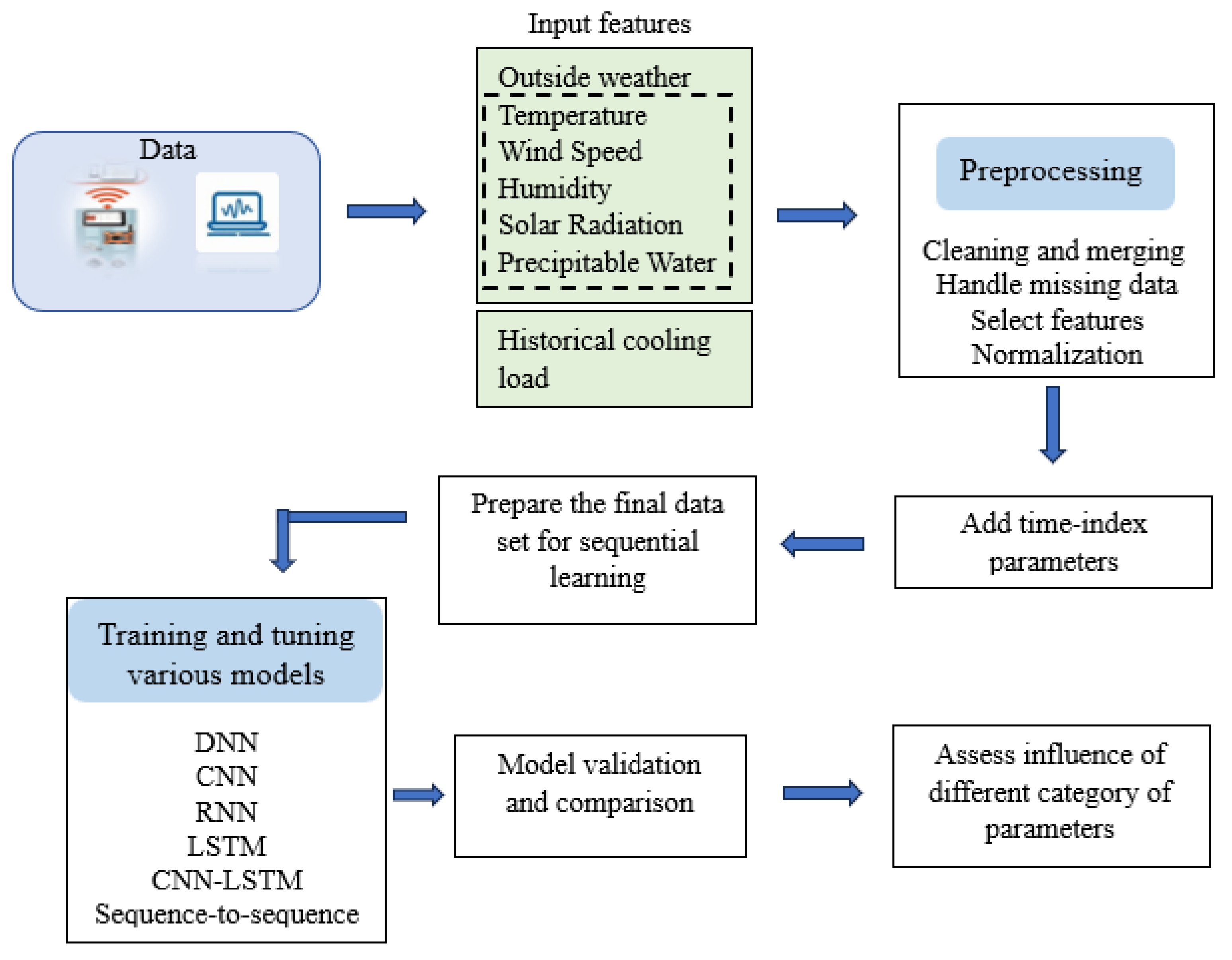
The overall research methodology is depicted in Figure 1. The first step comprises data collection from various sources like building management systems, simulations, and external weather sources. External weather parameters, including temperature, relative humidity, wind speed, solar radiation, and precipitable water, are collected from the Solcast website [34]. As data from diverse sources had different time scales, cleaning and merging them to make an hourly dataset constitutes the first step in data preprocessing [35]. Due to instrumental faults, a few days had missing entries in the real-world datasets. Removing those days from the respective datasets makes 0.7% of the data missing for the SIT@Dover dataset and 0.95% of the data missing for the SIT@NYP dataset. Since this percentage is very low, removing the corresponding days from the dataset has a negligible effect on prediction. Historical cooling load is calculated by extracting the building management system’s flow rates, chilled water supply, and return temperatures.

3.1. Feature Selection

After cleaning, merging, and handling missing data, an exhaustive analysis is performed to select the features required for prediction. A correlation analysis is performed to understand the importance of different input parameters on cooling load. The total parameters available for the analysis are outdoor temperature (Temp), relative humidity (Hum), wind speed (wSpeed), solar radiation (sRad), precipitable water (pWater), and cooling load (cLoad). The cross-correlation coefficient is used to quantify the influence of the lag of different input parameters on cooling load prediction. This measure gives an important inference on the variables to be selected for prediction and the historical time horizons that are more important in prediction. Figure 2 shows the cross-correlation values computed for different parameters for the three available datasets—SIT@Dover, SIT@NYP, and the simulated dataset.

As can be observed from these figures, precipitable water has very little influence on cooling load, with negligible cross-correlation values. All the other features are selected from the outdoor weather features category. The cross-correlation graph shown as ‘cLoad’ in these figures represents the lag effect and influence of the cooling load parameter on itself. This parameter has the highest cross-correlation values and is the most important in cooling load prediction.

Time index parameters are added to the dataset after this analysis. Hour-of-the-day and day-of-the-week are time index parameters, termed calendar features in this work. Previous studies reported that calendar features can substitute occupancy information when explicit occupancy data is unavailable. Different combinations of these parameters are tried for feature selection. The analysis is wound up with the parameters chosen for prediction, as enclosed in

Table 2. Parameters selected after analysis.

Category	Features
Outside weather features	Temperature, solar radiation, wind speed, relative humidity
Calendar features	Hour-of-the-day, day-of-the-week
Cooling load	Historical cooling load

. The subsequent experiments and comparisons are performed by using this selected feature set.

3.2. Normalization and Data Preparation

As can be observed from Table 2, a total of seven input features are selected for the prediction task. This refined dataset is passed through a normalization process. Normalization brings all the features to a standard scale of 0 to 1, making prediction model convergence easy and fast. This process is done as per Equation (1).

$$x_i^{\prime }=\frac{x_i-x_{min}}{x_{max}-x_{min}}$$

(1)

where $x_i$ is the ith sample, $x_{min}$ and $x_{max}$ are the minimum and maximum values for that feature and $x_i^{\prime }$ is the normalized value.

The next step entails preparing the dataset for different learning tasks, as each might need a slightly different treatment of the input data. For example, Deep Neural Networks require input data in a two-dimensional shape. Data can be fed in format (x,y) where x is the input feature vector of shape Nxd and y is the output vector of shape Nxh. Here, N denotes the number of samples in the dataset, d is the dimension of the input, and h is the number of hours of the next day being predicted. Data is converted to three-dimensional input and complementary target samples to cater to deep learning models. The input dataset has the shape NxTxd, and the target dataset has the shape Nxhx1, where T denotes the number of historical hours given as input to the model. For example, if 12 h of data from the daytime of the previous two days is given as input to the model, then $T=24$.

3.3. Prediction Models

To perform an extensive comparison of the ascendancy of various deep learning models in day-ahead cooling load prediction, four standalone models and two hybrid models are implemented in this work. DNN, CNN, RNN, and LSTM are the standalone models, while CNN-LSTM and sequence-to-sequence are the hybrid models. A brief description of each of these learning algorithms is given in the sub-sections below.

3.3.1. Deep Neural Network

Deep neural networks have a layered architecture. It is like Artificial Neural Networks in terms of their functioning and architecture, but the difference mainly comes from the number of layers added to make the network ‘deep’. Each layer helps the network to extract higher-level features. Unlike conventional neural networks, DNNs can add more densely connected layers, each of which can use different activation functions if required. Its agility in adding dropout layers makes it superior to the ANN architecture [8]. This feature makes it capable of randomly dropping a percentage of neurons from any layer, consequently avoiding overfitting. The input layer accepts the input, hidden layers process the input to extract higher-level features, and finally, the output layer provides the output. This network can be used as a multi-output model. Depending on the number of neurons in the output layer, the multi-output feature can be easily tailored to this architecture.

3.3.2. Convolutional Neural Network

A convolutional neural network is a kind of deep learning network with a feed-forward structure. They use kernels or filters to process the input, which slide over the input and compute the cross-correlation between the kernel and each part of the input. This way, highly correlated input parts get more weightage. This method was originally built for image processing tasks but nowadays found successful in time series regression problems like load prediction [26,36,37]. In addition to the input, convolution, and pooling layers, CNN can have dense layers at the network’s end. This architecture makes it suitable for prediction tasks. With a suitably designed dense layer at the end, multi-output prediction is also possible with this network. Upon removal of the eventual dense layer, the same architecture serves the purpose of a feature extractor. Higher-level features can be extracted from the input depending on the size of the kernels used in filtering.

When used as a standalone model, CNN follows its conventional architecture with a dense layer at the end. Convolution layers can be one-dimensional or two-dimensional, the selection commensurate with the shape of the filter. One dimensional convolution layer requires only the length of the filter to be mentioned, whereas the width is automatically set equal to the width of the input data set. Width, in this case, refers to the number of features in the dataset. Conversely, a two-dimensional convolution layer works with a two-dimensional kernel, usually mentioned as 2 × 2, 3 × 3, or 5 × 5. Convolution layers extract higher-level features from the input data, which helps to provide better predictions.

3.3.3. Recurrent Neural Network

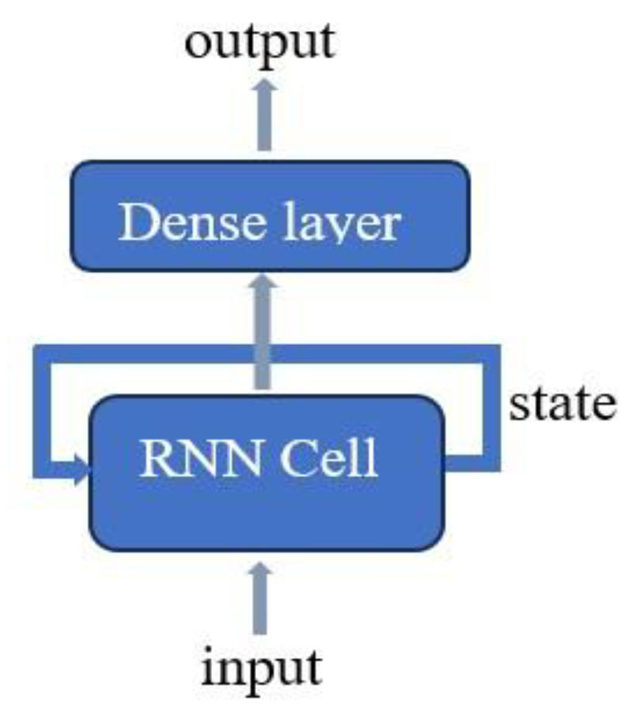
Recurrent neural networks have a structure different from the feed-forward neural networks. In feed-forward networks, input flows in the forward direction only, whereas, in recurrent neural networks, recurrent connections are possible, which means that output from an internal node can impact the subsequent input to the same node. These recurrent connections make this network suitable for learning from sequential data like time series. The basic architecture of an RNN is depicted in Figure 3.

A recurrent neural network cell has multiple fixed numbers of hidden units, one for each time step of the network processes. Each unit can maintain an internal hidden state, representing the unit’s memory regarding the sequential data. This hidden state is updated at each timestep to reflect the changes in the sequential data. Hidden state update is done as per Equation (2).

$$h_t=f(W_h{h}_{t-1}+W_x{X}_t+b_h)$$

(2)

where $h_t$ is the vector representing h, the hidden state at time t, W_x denotes the weights associated with inputs, W_h is the weights associated with hidden neurons, X_t is the input vector, $b_h$ is the bias vector at the hidden layer. $f$ denotes the activation function used at the hidden layer. Based on the number of inputs and outputs, RNN can be configured as one-to-one, one-to-many, many-to-one, or many-to-many. In this work, the RNN takes multiple time steps as input and produces multiple time steps as output. Hence, it is used as a many-to-many network.

3.3.4. Long Short-Term Memory

Long short-term memory (LSTM) is an advanced, recurrent neural network specially designed to contend with the problem of vanishing gradients [38]. With the help of a cell and three gates as the basic building blocks, it enhances the memorizing capability of recurrent neural networks. These three gates are termed input, output, and forget gates. LSTM network can memorize thousands of time steps, making it suitable for handling time series problems. The gates regulate the flow in and out of the cell state. The input gate regulates the input flow to the memory cell and decides what latest information will be added to the current state. The output gate determines what information from the memory cell will be passed to the output. Conversely, the forget gate helps to decide what information is to be discarded or forgotten from the current state. The LSTM network efficiently forgets the old or irrelevant information with the forget gate. In short, LSTM can discriminatively maintain or discard information as the data flows through the network, which makes it suitable for learning long sequences. LSTM performs its work with the following four steps.

Step 1: Output of the forget gate, $f_t$ is calculated in the first step.

$$f_t=\sigma \left(w_f\left[X_t,Y_{t-1}\right]+b_f\right)$$

(3)

where $w_f$ and $b_f$ denote the weight and bias vectors at the forget gate, respectively. $X_t$ is the input at the current iteration, $Y_{t-1}$ is the output from the previous iteration, and σ is the activation function.

Step 2: The cell state output $C_t^{\prime }$ and the output of the input gate $i_t$ are calculated.

$$C_t^{\prime }=a_i\left(w_c\left[X_t,Y_{t-1}\right]+b_c\right)$$

(4)

$$i_t=\sigma \left(w_i\left[X_t,Y_{t-1}\right]+b_i\right)$$

(5)

Here, $a_i$ is the input activation function, $w_c$ and $b_c$ are the weight and bias vectors of the cell state, $w_i$ and $b_i$ are the weight and bias vectors at the input gate.

Step 3: The cell state value $C_t$ is updated in this step.

$$C_t=i_t.C_t^{\prime }+f_t.C_{t-1}$$

(6)

Step 4: The output of the output gate, cap O sub t, s calculated in this step. This gate combines previous iterations’ output $Y_{t-1}$ and the current input $X_t$, using $b_o$ as the bias and $w_o$ as the weight vector. Finally, the output $Y_t$ is computed.

$$O_t=\sigma \left(w_o\left[X_t,Y_{t-1}\right]+b_o\right)$$

(7)

$$Y_t=O_t.a_o\left(C_t\right)$$

(8)

3.3.5. CNN-LSTM

Convolutional neural networks and long short-term memory are connected sequentially to make a hybrid structure [39]. The structure of this hybrid model is shown in Figure 4. CNN is used as a feature extractor here. During the initial feature selection process, it was identified that the historical cooling load is the most influential parameter in prediction. Hence, extensive experiments are conducted to analyze what combination of inputs to CNN and LSTM enhances the results. Through experiments, it is concluded that the hybrid model provides maximum performance when the inputs, excluding cooling load, are given as input to the CNN. More informative features are extracted from these input parameters using CNN. Then, the extracted features are combined with the original cooling load features before being provided as input to the LSTM model. This process is shown in Figure 4.

The outputs of the LSTM network are processed by a dense layer to finally obtain the desired multi-step prediction. One-dimensional and two-dimensional convolution layers are tried on CNN. The LSTM can consider the sequential behavior of historical cooling load as the cooling load is given in raw form to the LSTM network, without passing through the CNN. The configuration of the CNN-LSTM model used for processing the SIT@Dover dataset in this work is shown in

Table 3. Configuration of CNN-LSTM network.

Layer	Size
Input1	T × (D − 1)
Input2	T × 1
Convolution1, 2	Feature size = 16, kernel size = 2 activation = tanh
Convolution 3, 4, 5, 6	Feature size = 16, kernel size = 3 activation = tanh
Convolution 7	Feature size = 48, kernel size = 3 activation = tanh
Reshape	T × -
Concatenate	Output of Reshape and Input2
LSTM	Number of units = 128, activation = tanh
Dense	Number of units = h

. The number of features and the kernel size at each convolution layer are set in an ascending order, as depicted in the table. One-dimensional convolution gives better performance compared to two-dimensional convolution.

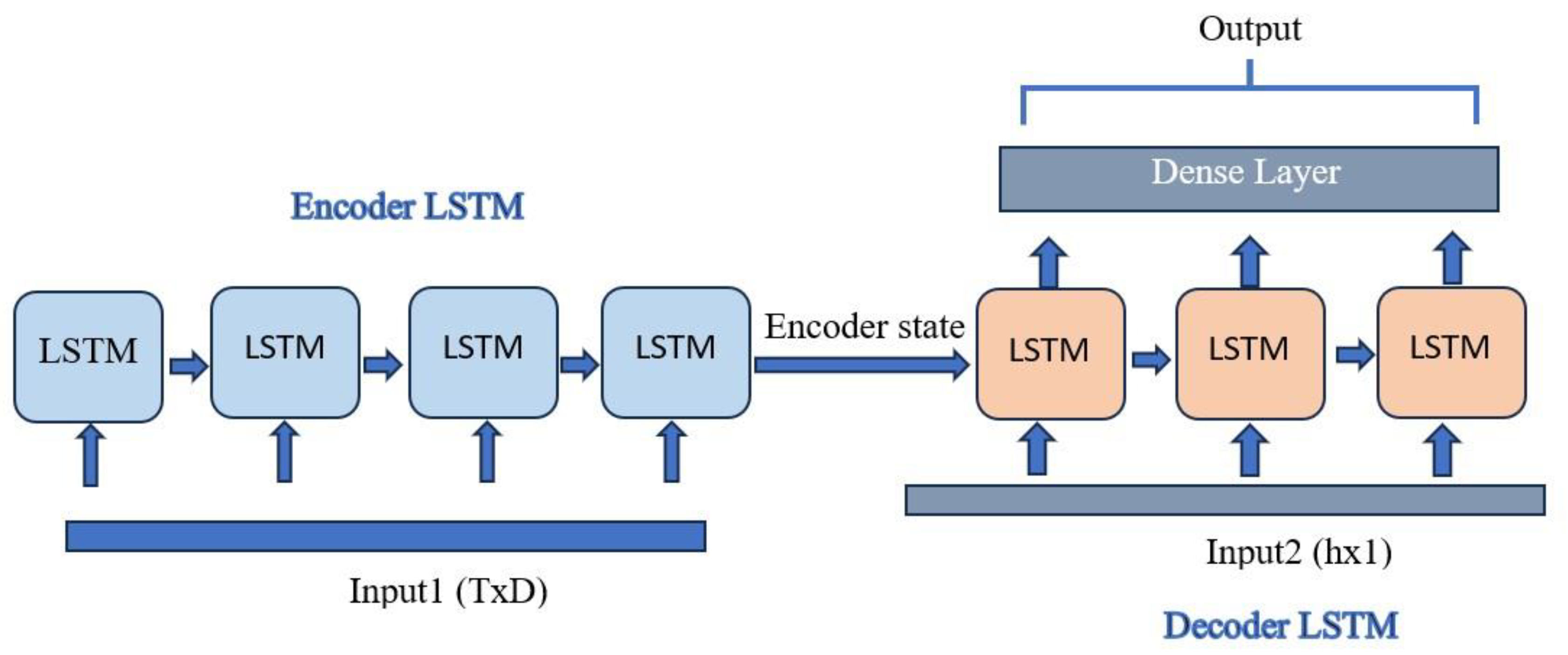
3.3.6. Sequence-to-Sequence

The sequence-to-sequence model, also known as the encoder–decoder model, combines two LSTM networks, the first for encoding the information in the input sequence and the second for generating the output sequence. A dense layer is connected at the end of the LSTM network to take multi-step prediction as output. Encoder LSTM passes its hidden and cell states to the decoder; hence encoded information. The encoder and decoder can have diverse configurations, including the number of hidden units, activation functions, and other parameters. Both LSTM networks use 64 hidden neurons and ‘tanh’ as the activation function in this work. The final dense layer has ‘h’ neurons and ‘linear’ activation is used. The encoder’s return state is set to true to retrieve the hidden state information from the encoder.

In addition to the state information retrieved from the encoder, decoder LSTM can take separate input from outside, noted as input2 in Figure 5. Generally, on the decoder side, the output of previous LSTM units can be given as input to the consequent LSTM unit. Another alternative option is to provide ground truth information as input to the decoder. This method is known as teacher forcing and is usually prevalent in language processing models. Teacher forcing ensures fast and effective training of the model. A problem associated with this method is that it might cause errors while using a model trained this way in real scenarios for prediction. The model might confront unforeseen sequences in real prediction scenarios. In this work, providing the ground truth as input to the decoder is not realistic; hence, an alternate option is adopted. The most similar day’s load sequence is given as input to the decoder from the historical cooling load series. During correlation analysis, it is observed that the time lags resemble the target load sequence, the previous day’s load sequence and the previous week’s same day’s load sequence. Experiments revealed that the previous week’s and the same day’s load sequences give better results instead of the previous day’s load sequence. Hence, this load sequence is given as input to the decoder model.

To summarize, this section overviews the deep learning algorithms used in this study. The formation of hybrid models is discussed in detail. A dense neural network layer is added as the last layer in all the above-mentioned deep learning networks. This layer enables the models to provide multiple outputs naturally. The whole multi-step prediction is treated as a single independent problem, which is solved in a non-recursive way. Inferences drawn from the correlation analysis are used to customize the models by deciding the input combinations suitable at various stages of the models. The CNN-LSTM model is improvised by dividing the input features into two separate sets—the first set, including all features except cooling load, is given to the CNN for extracting higher-order features, and the second set, including these extracted features and the cooling load series, is given to the LSTM network. The default sequence-to-sequence model is improvised by providing the previous week’s same-day cooling load series as the teacher forcing input at the decoder stage.

3.4. Performance Metrics

The performance evaluation metrics are carefully chosen to epitomize an extensive validation and comparison of the developed models. To ensure the reliability of results, 10 trial runs are conducted for each experiment, and the performance measures are averaged over these trials. Root Mean Squared Error (RMSE), Coefficient of variation of Root Mean Squared Error (CV-RMSE), Mean Absolute Percentage Error (MAPE), and Mean Absolute Error (MAE) are the performance metrics selected in this work. The computation of these metrics can be found in Equations (9) to (12).

$$\mathrm{R}\mathrm{M}\mathrm{S}\mathrm{E}=\sqrt{\frac{1}{\mathrm{N}}{\displaystyle {\sum }_{\mathrm{i}=1}^{\mathrm{N}}}{\left({\mathrm{y}}_{\mathrm{i}}^{\prime }-{\mathrm{y}}_{\mathrm{i}}\right)}^2}$$

(9)

$$\mathrm{C}\mathrm{V}-\mathrm{R}\mathrm{M}\mathrm{S}\mathrm{E}=\frac{\sqrt{\frac{1}{\mathrm{N}}{\displaystyle {\sum }_{\mathrm{i}=1}^{\mathrm{N}}}{\left({\mathrm{y}}_{\mathrm{i}}^{\prime }-{\mathrm{y}}_{\mathrm{i}}\right)}^2}}{\frac{1}{\mathrm{N}}{\displaystyle {\sum }_{\mathrm{i}=1}^{\mathrm{N}}}{\mathrm{y}}_{\mathrm{i}}^{\prime }}$$

(10)

$$\mathrm{M}\mathrm{A}\mathrm{P}\mathrm{E}=\frac{1}{\mathrm{N}}{\displaystyle {\sum }_{\mathrm{i}=1}^{\mathrm{N}}}\frac{\left|{\mathrm{y}}_{\mathrm{i}}^{\prime }-{\mathrm{y}}_{\mathrm{i}}\right|}{{\mathrm{y}}_{\mathrm{i}}}\times 100\mathrm{\%}$$

(11)

$$\mathrm{M}\mathrm{A}\mathrm{E}=\frac{1}{\mathrm{N}}{\displaystyle {\sum }_{\mathrm{i}=1}^{\mathrm{N}}}\left|{\mathrm{y}}_{\mathrm{i}}^{\prime }-{\mathrm{y}}_{\mathrm{i}}\right|$$

(12)

where N is the number of samples in the test set, $y_i^{\prime }$ is the predicted value and $y_i$ is the original value of the i^th sample in the test set.

4. Results and Discussion

Experiments are conducted on a Windows 11 machine with an Intel(R) Core (TM) i7-12650H Processor and 64 GB physical memory. PyCharm Integrated Development Environment is used for implementing prediction models, whereas the Keras deep learning library on the TensorFlow platform (version 2.12.0) functioned as the supporting software platform.

4.1. Data

Three datasets are used in the experiments; two of them are authentic building datasets, and the third one is a simulated dataset. The buildings are educational institution buildings in Singapore. The first dataset pertains to a single office floor in the SIT@Dover building, referred to as the SIT@Dover dataset in this paper. Attributable to the fact that this dataset is limited to a single office floor, the range of cooling load values is comparatively narrower. The maximum recorded cooling load value in this dataset is 43 kW. This building has a 75F building management system implemented, making data collection easier. The data spans from 1 January 2023 to 7 July 2023 and was recorded at 1 h intervals. Holidays are not considered while preparing the dataset. Since this office works only during the daytime, the data between 7 a.m. and 6 p.m. is considered here, making a total of 1524 samples in this dataset.

The second real dataset, the ‘SIT@NYP dataset’, is collected from another institutional building in Singapore, the SIT@NYP building. This dataset has a wider range of cooling load values, spanning an entire building with seven floors. The highest cooling load recorded within this dataset is 1525 kW. Considering the working hours of the building, holidays are excluded, and only the data from 8 a.m. to 6 p.m. is selected for experiments. Datasets are aggregated into hourly data to prepare for training. The dataset spans 1 May 2022 to 30 September 2022, encompassing 1144 individual samples.

The Integrated Environmental Solution Virtual Environment (IESVE) software (version 2022) simulates the third dataset. The simulated space corresponds to the Co-Innovation and Translation Workshop Room on the 16th floor of the innovative Super Low-Energy Building, overseen by the Building Construction Authority in Singapore. The simulation model incorporates input variables encompassing outdoor and indoor design conditions, including location, space, and weather data. Temperature, relative humidity, internal heat gain, and the factors attributed to occupants, lighting, and computers are the input attributes considered. This dataset comprises one year of data collected at 1 h intervals, but only day hours from 9 a.m. to 6 p.m. are considered; hence, it totals 3650 samples. A summary of the datasets is given in

Table 4. Summary of the datasets.

	SIT@Dover Dataset	SIT@NYP Dataset	Simulated Dataset
Duration	6.5 months	5 months	1 year
The time interval of data	hourly	hourly	hourly
Number of samples	1524	1144	3650
Maximum load	40.58	1525	20.76
Minimum load	10.18	295	10.29
Mean	31.63	806	16.72
Standard deviation	5.15	168	1.97

. The maximum value, minimum value, mean, and standard deviation are given in kW.

Train and test sets are derived from the datasets by keeping the sequential order unperturbed. For the SIT@Dover dataset, data from 1 January to 15 June 2023 is considered the training set, and the rest is used to create the test set. Similarly, for the SIT@NYP dataset, the training set corresponds to the period from 1 May to 9 September 2023; for the simulated dataset, the training set corresponds to 1 January to 30 November 2022.

4.2. Tuning Hyperparameters of Models

For all the models, ‘Adamax’ performs the function of the optimizer. This conclusion is drawn after comparing it with the other optimizers like Adam, SGD, and RMSprop. A learning rate of 0.001 is chosen from the set [0.1, 0.01, 0.001]. Compared to mean squared error, mean absolute error is found to provide better results when used as a loss function in learning, and hence, the models are implemented with this loss function. Consistently among all the models, the number of hidden units used in the final dense layer is determined based on the number of hours of the next day to be predicted.

Experiments are conducted for the Deep Neural Network to compare the effect of increasing the number of hidden layers. It is found that a single hidden layer with 1024 hidden neurons provides better results. Increasing the number of neurons or hidden layers further did not improve the results. This may be attributed to the fact that when the number of layers or neurons increases, the total number of hyperparameters to be learned also increases, consequently leading to overfitting.

For convolutional neural networks, the number of convolution layers and the filter size are tuned based on the dimension of the input data. For the SIT@NYP and simulation datasets, six convolution layers are used, whereas for the SIT@Dover dataset, seven convolution layers are used. RNN and LSTM networks use single hidden layers with 64 neurons, a decision taken after comparing the performance rendered with more hidden layers and hidden units.

The CNN-LSTM hybrid model structure used in this paper necessitates tuning the number of layers and the filter size based on the dimension of the input data. It is done in the same way as discussed earlier for the standalone CNN model. The LSTM network in this hybrid model uses 64 hidden neurons. For the sequence-to-sequence model, both the encoder and decoder LSTM models have 64 hidden nodes.

4.3. Decision on Time Horizons to Be Given as Input

Depending on the time horizons selected as input from the historical data, the prediction accuracy of different models can vary. Identifying the most informative time horizons is found crucial. The cross-correlation coefficient is a statistical method that implies the correlation between the target variable and the time lags of the independent variables. It helps decide the time lags more correlated to the target variable, and the input selection enhances the prediction accuracies. The correlation analysis showed that the immediate previous one or two days and the similar two days of the previous week give relatively better scores for the correlation coefficient. However, providing too many historical time horizons might lead to overfitting and loss of generalizability of the model.

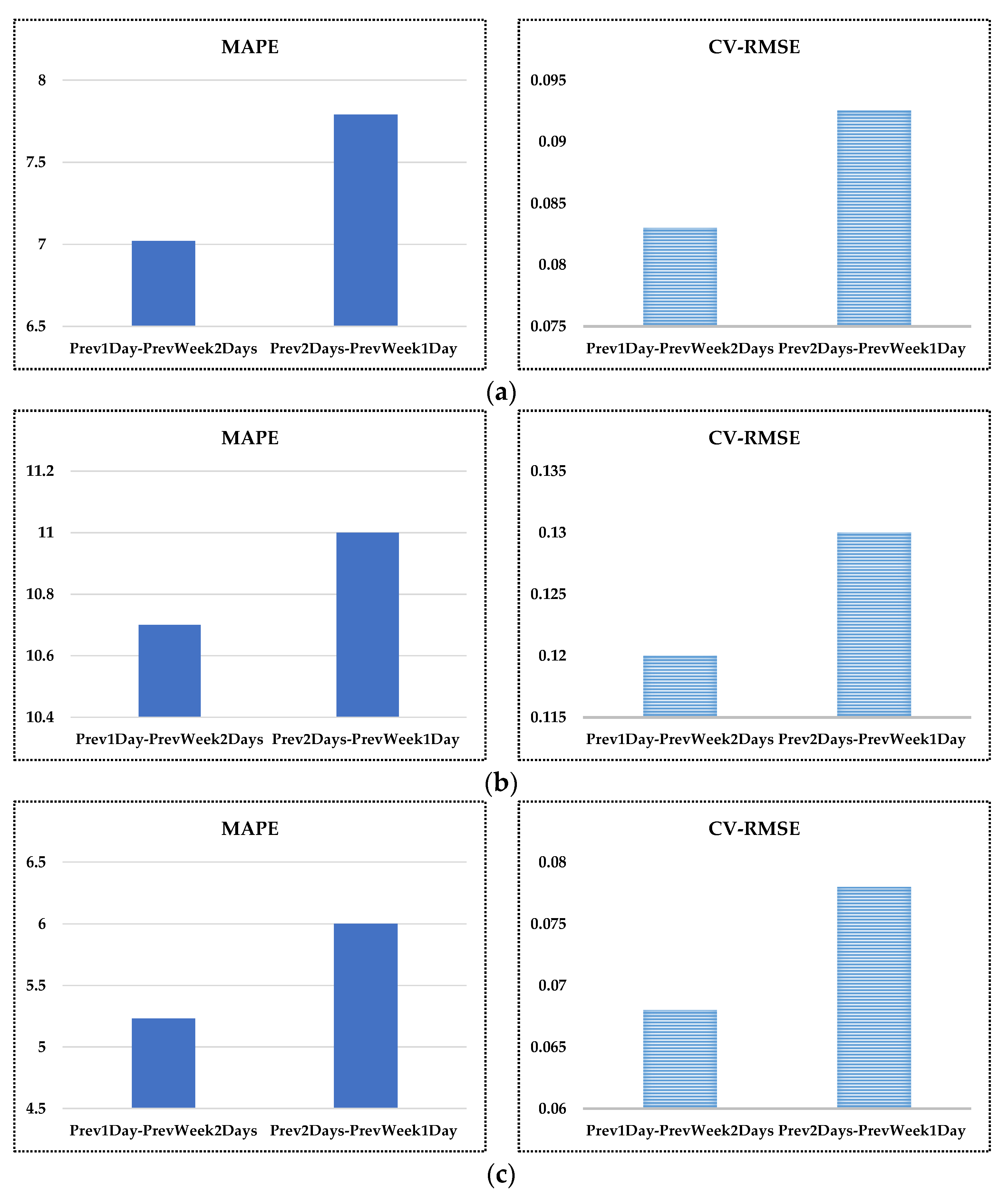
Hence, a study determined the relative performance of two sets of input time horizons. Two sets of experiments are carried out to choose the most relevant inputs from these time horizons. LSTM, one of the base models with all three datasets, has been selected to perform this comparison. In the first set of experiments, data from the previous day, the same day of the previous week, and the day before that are taken. This set is denoted as ‘Prev1Day-PrevWeek2Days’ in Figure 6. The second set of experiments considers the previous two days and the same day of the previous week, denoted as ‘Prev2Days-PrevWeek1Day’ in the figure. Performance comparison between these two sets of experiments is depicted in Figure 6. MAPE and CV-RMSE values obtained for different datasets can be seen in the figure. As can be observed from the figure, all the performance measures agree on the fact that the set ‘Prev1Day-PrevWeek2Days’ outperforms the other version. The improved performance of the selection ‘Prev1Day-PrevWeek2Days’ can be attributed to the fact that this set helps to capture the relation between the day to be predicted and the previous day using the previous week’s data. This information is lacking in the other set. Hence, the paper follows this time horizon selection as input to the model.

4.4. Results

The comparative performance of all six models is assessed through experiments. The datasets are transformed into samples with shapes suitable for different models. The input samples are formed by joining historical data samples, as discussed in the above section. Data from the previous day and the previous week’s two days make a total of 3 × h rows in each sample. Thus, the number of historical hours given as input to the model is T = 3 × h. This value comes out to be 36 for the SIT@Dover dataset, 33 for the SIT@NYP dataset, and 30 for the simulated dataset. DNN requires a flattened data structure as input to the model. Hence, T hours, each with seven features, make a total of 252 features for the SIT@Dover dataset, 231 features for the SIT@NYP dataset, and 210 features for the simulated dataset. In the cases involving deep learning models, the input samples must have a three-dimensional structure of shape N × T × D, where N is the number of samples, T is the number of hours, and D equals the number of input features. A comparison of the performance offered by various models on different datasets under consideration can be seen in

Table 5. Performance metrics computed for various models.

	Model	RMSE	CV-RMSE	MAPE	MAE
SIT@Dover	DNN	3.02	0.097	7.87	2.46
	CNN	2.88	0.090	7.64	2.38
	RNN	2.94	0.091	7.53	2.33
	LSTM	2.66	0.083	7.02	2.15
	CNN-LSTM	2.63	0.082	6.71	2.03
	Seq-to-seq	2.38	0.074	6.26	1.8
SIT@NYP	DNN	99.13	0.13	11.84	73.41
	CNN	103.84	0.13	12.26	73.92
	RNN	95.90	0.12	11.3	68.17
	LSTM	91.54	0.12	10.79	62.24
	CNN-LSTM	93.18	0.12	11.11	65.39
	Seq-to-seq	84.5	0.1	9.8	55.21
Simulated dataset	DNN	1.19	0.07	5.71	0.87
	CNN	1.1	0.069	5.34	0.82
	RNN	1.08	0.068	5.17	0.79
	LSTM	1.08	0.068	5.23	0.79
	CNN-LSTM	1.11	0.07	5.43	0.82
	Seq-to-seq	0.99	0.06	4.76	0.72

.

As the performance metrics quoted in Table 5 depict, the sequence-to-sequence model offered the best performance for all three datasets. When a second LSTM network is added to make a sequence-to-sequence architecture, and the most matching load sequence from the history is given as external input to the decoder LSTM, the performance gets boosted. An extensive examination is conducted to check the performance variations when providing various combinations of inputs at the encoder and decoder sides. The input, as mentioned above, selection is found to be the most reliable. DNN, CNN, and RNN offered the least relative performance on all the datasets. While comparing the performance of the base deep learning architectures—DNN, RNN, CNN, and LSTM—LSTM offered consistently better performance on all the datasets under consideration. This superior performance of LSTM is attributed to its competence in handling the vanishing gradients problem and memorizing long sequences.

While comparing CV-RMSE and MAPE values for all the models across all three datasets, it can be observed that the highest level of performance is achieved for the simulated dataset, followed by the SIT@Dover dataset and the SIT@NYP dataset. This performance trend can be attributed to the inherent differences in the dataset’s characteristics. The simulated dataset, generated by software, presents the least challenge due to its controlled nature. In contrast, SIT@NYP and SIT@Dover datasets are derived from real-world sources, with SIT@NYP posing a greater challenge than SIT@Dover. The SIT@NYP dataset has higher values and higher standard deviation for cooling load, rendering it more complex for predictive models compared to the other datasets.

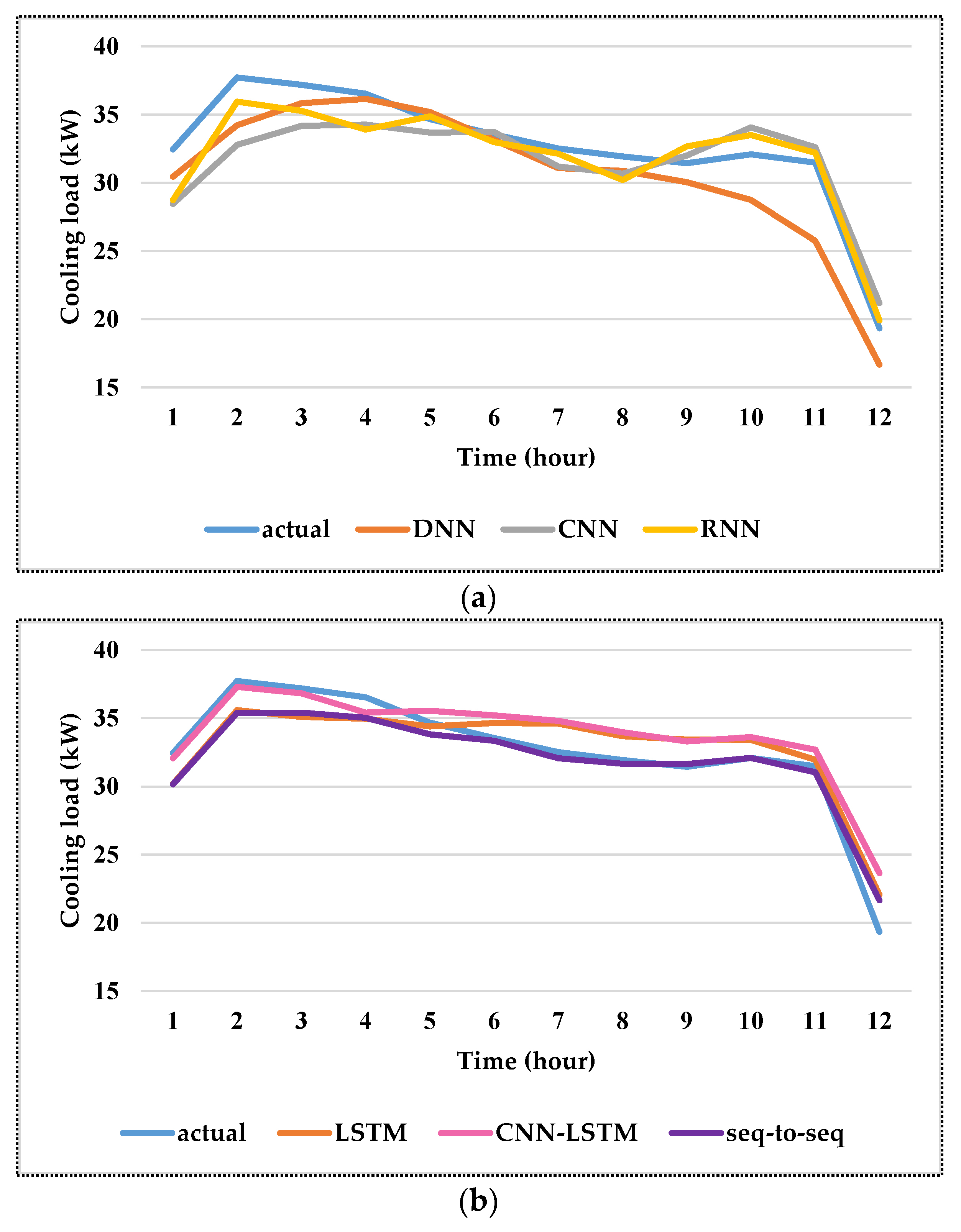
One of the datasets and a randomly selected date are chosen to show the cooling load predictions in detail. Due to space considerations and to avoid presenting repeating information, the other datasets are not considered here for presenting detailed cooling load and error plots. An example of 12 h cooling load predictions done by various models for the SIT@Dover dataset has been shown in Figure 7. The example day corresponds to Wednesday, 5 July 2023. A normal working day is chosen as the example day to show the predictions done by various deep learning models. Figure 7a depicts the DNN, CNN, and RNN predictions, while Figure 7b shows LSTM, CNN-LSTM, and sequence-to-sequence models. Overall, the second set of models, LSTM, and the two hybrid models derived from LSTM showed better performance than DNN, CNN, and RNN. In addition, while comparing the LSTM-derived models, the sequence-to-sequence model prediction better matched the actual load.

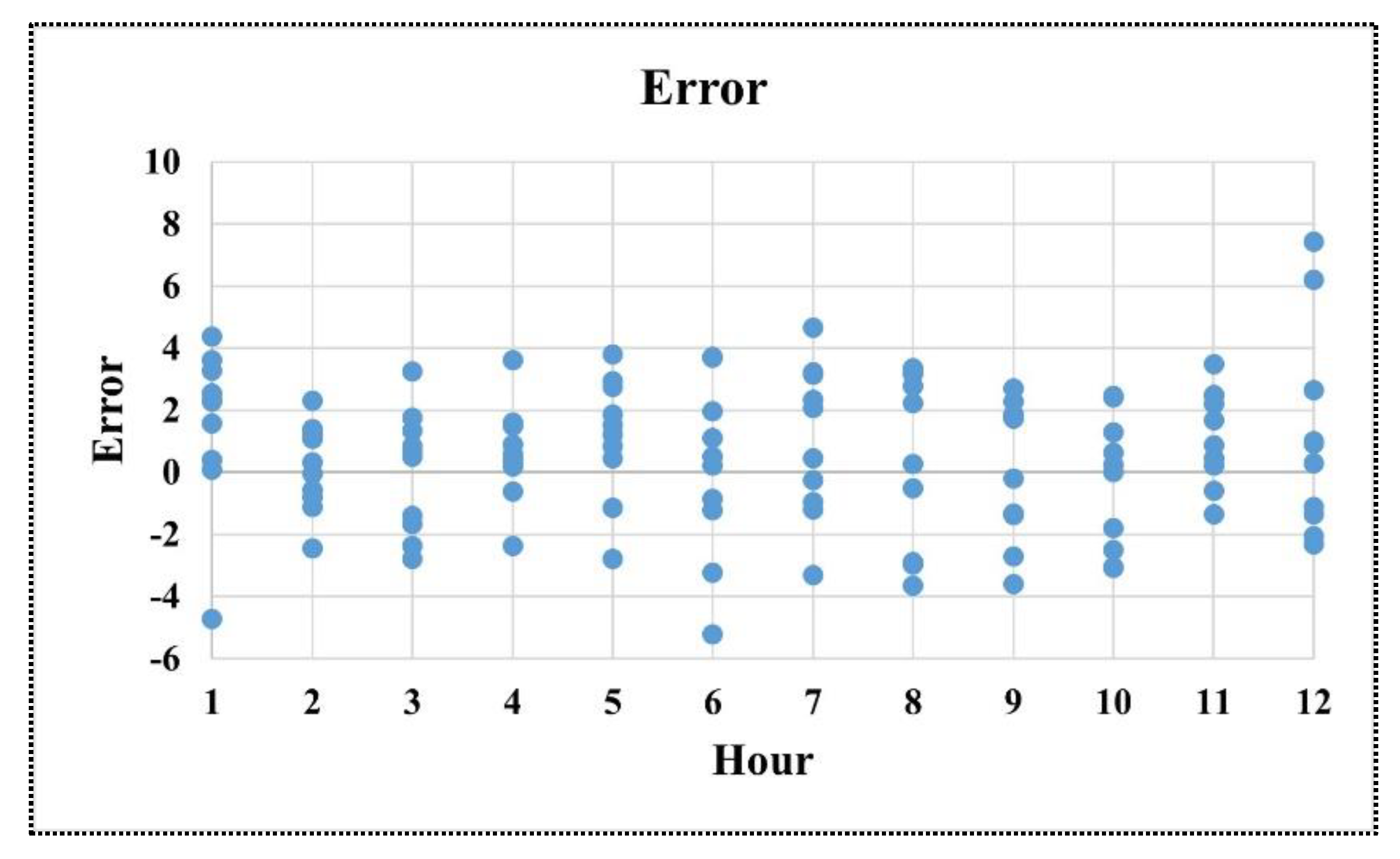
Figure 8 shows the error computed between the actual and predicted cooling loads by the sequence-to-sequence model for the SIT@Dover dataset. This figure shows that the first, last, and lunch hours have the highest errors. While analyzing the general trend in error distribution, it is observed that the highest error values occur during the hours when the load values are lower. In addition, while comparing the first half of the day with the second half, the error is more in the afternoon hours, and the same trend follows generally on all days. This error is mainly attributed to the fact that explicit occupancy information is missing in the dataset, and the general trend of people leaving the office in the afternoon hours can be captured only if the actual occupancy information is available. This emphasizes that occupancy data has an equivalent role in prediction accuracy as external weather parameters, and the absence of this information can be crucial in the prediction model’s performance. Even though calendar features can give hints on occupancy patterns, this information has limitations in real predictions.

4.5. Validating the Importance of Various Categories of Parameters

Experiments are conducted to assess the influence of various groups of parameters on prediction performance. Only those categories included in the final dataset are considered in this experiment. ‘Outdoor weather parameters’ is one such category that contains outdoor temperature, solar radiation, wind speed, and relative humidity. ‘Calendar features’ included day-of-the-week and hour-of-the-day. Historical cooling load is the third category of parameters. The prediction performance reported in Table 5 corresponds to the input combining all these parameter categories. Each category is excluded individually in the present set of experiments, and the performance is validated. Figure 9 shows the RMSE and MAPE values computed by the Sequence-to-sequence model for the three datasets, excluding each category of parameters. ‘All-param’ denotes the normal case in which all three categories of parameters are included. The names ‘No-calendar’, ‘No-weather’, and ‘No-Load’ correspond to the cases when calendar features, outdoor weather features, and historical cooling load are excluded from the input list.

As can be observed from the plots in Figure 9, the best performance is obtained from the sequence-to-sequence model when all three categories of input parameters are combined in the input parameter list. Historical cooling load among the input features has the most influence on prediction performance; hence, removing it degrades the performance more. Calendar features have the next highest influence, followed by outdoor weather features. These results emphasize that occupancy information has more influence on cooling load prediction than external weather features in tropical climates, as mentioned in the introduction.

5. Conclusions

Compared to short-term cooling load predictions, such as hour-ahead load prediction, deep learning techniques are less attempted in day-ahead cooling load predictions. Day-ahead cooling load prediction falls into the category of multi-step prediction, which is more challenging than short-term single-step prediction. This paper applies advanced deep-learning techniques to predict the next day’s cooling load. Six deep learning architectures, including four single standalone models and two hybrid architectures, are attempted for long-term cooling load prediction. The selected algorithms represent distinct categories of deep learning architectures, like deep neural networks, recurrent neural networks, convolutional neural networks, and long short-term memory. Hybrid architectures are formed by combining CNN with LSTM and LSTM with LSTM; the latter is called the sequence-to-sequence model.

Experiments and results concluded that long short-term memory provided better results relative to the other single standalone models. Input, output, and forget gates in LSTM architecture help decide what information to forget and how much information to forward to the next steps. LSTM can remember long sequences due to the presence of these gates, which is especially useful in day-ahead hourly load predictions. LSTM combined with another LSTM as an encoder–decoder architecture enhances the prediction accuracy further. The results supported the idea that the sequence-to-sequence model is the best-performing model among all the deep learning models tried in this paper. Future work includes extending the present sequence-to-sequence model with an attention mechanism. Attention helps the network to focus on specific input combinations based on correlation. In addition to enhancing the model’s accuracy, it is also useful for improving the interpretability. The current work considered only buildings in tropical climates; its ability to generalize to buildings in other climate regions must be assessed in future work.