
Investigation of Building Profiles for the Energy Simulation of a Factory Building: A Case Study in South Korea

Abstract
1. Introduction
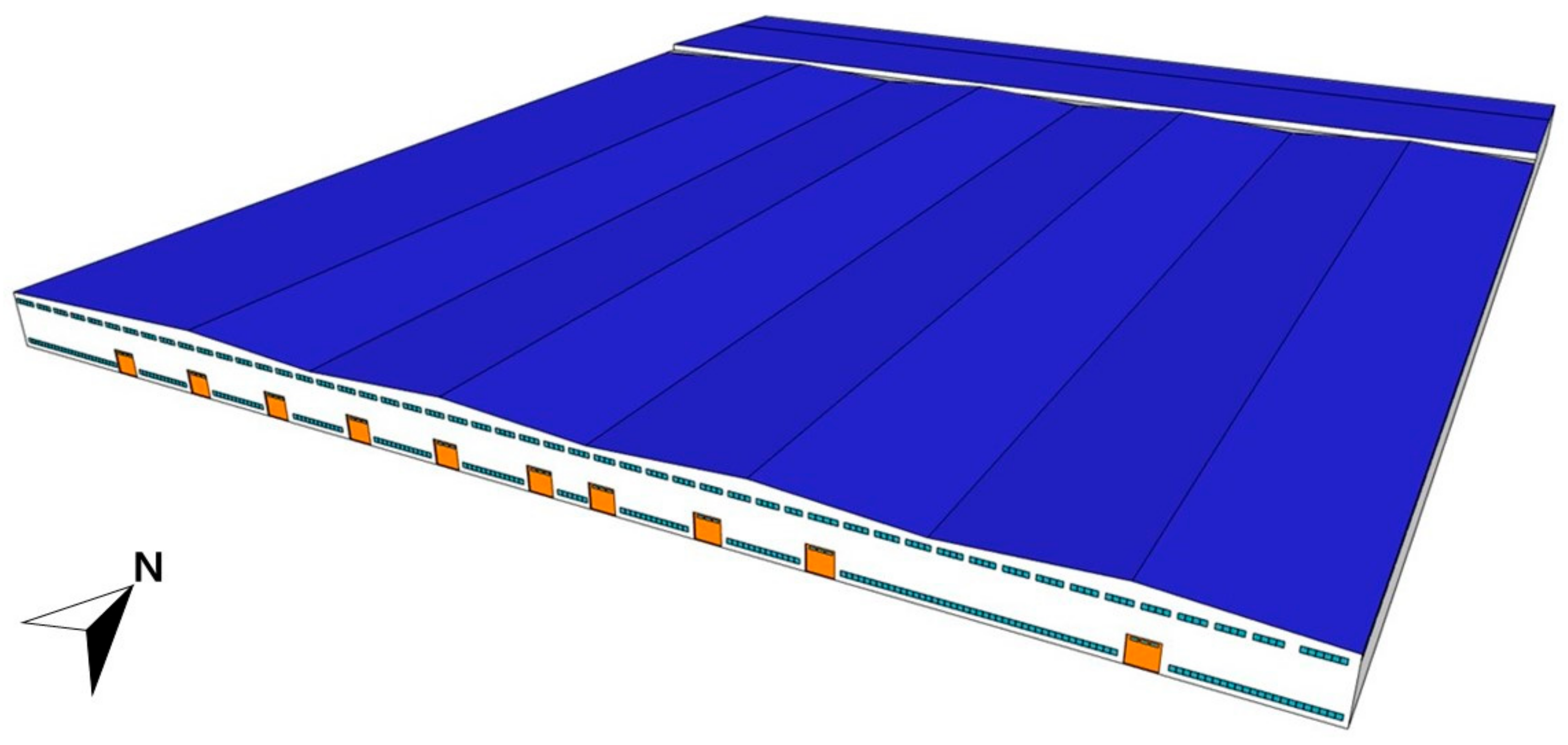
2. Target Factory Building
3. Building Profiles of the Factory Building
3.1. Field Data-Based Building Profiles
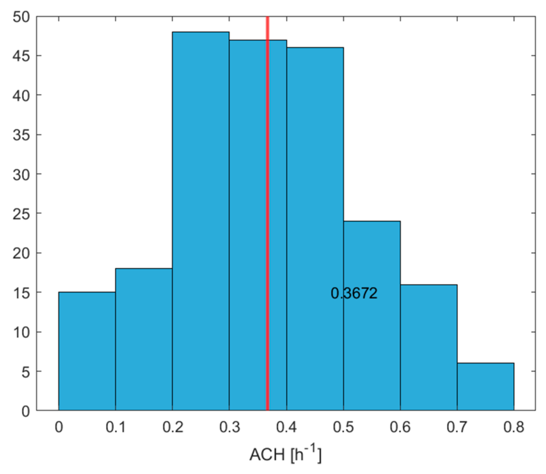
3.1.1. Air Change Rate
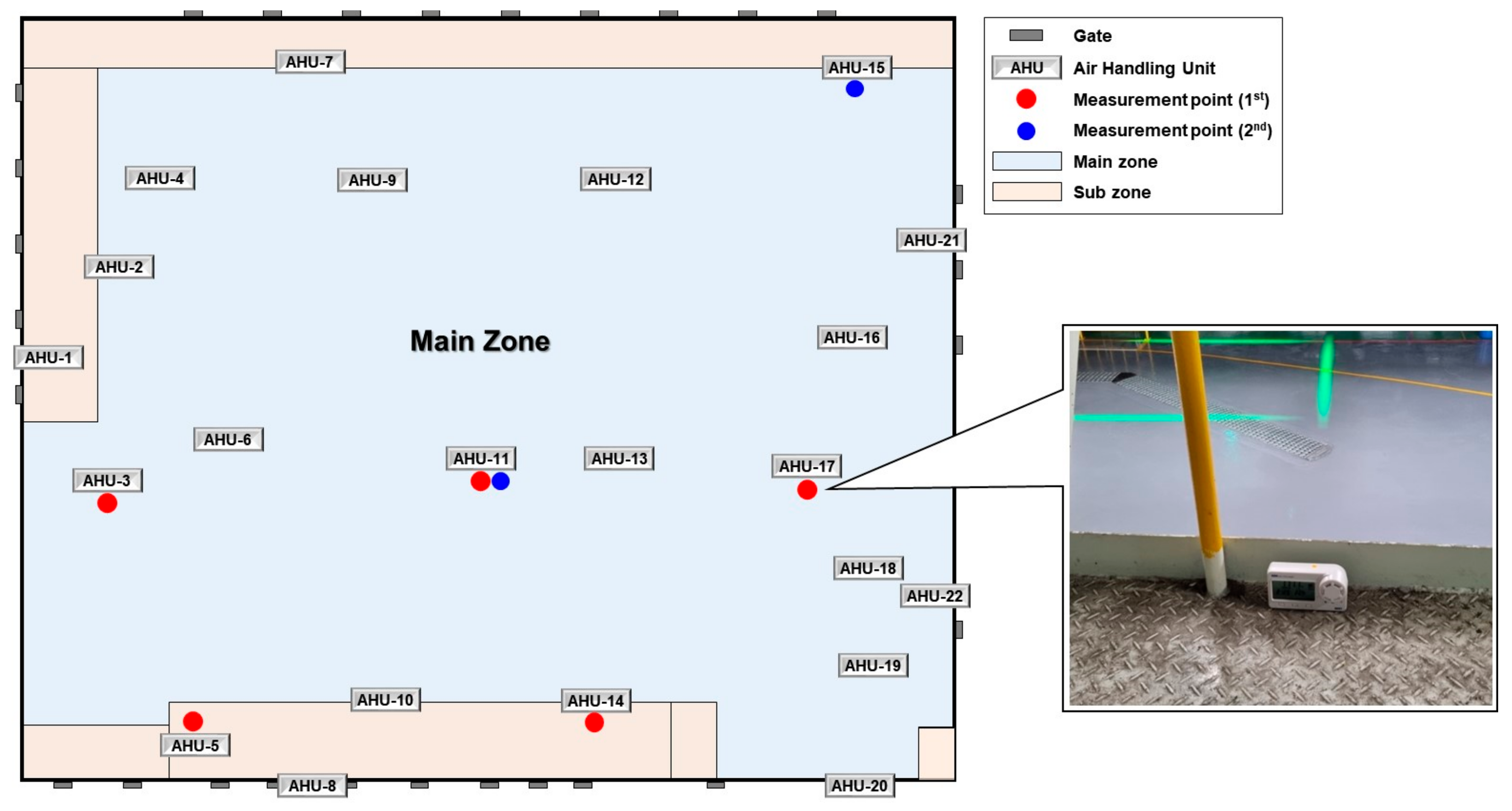
- Measurement setup
- 2.
- Analysis method
- 3.
- Air changes per hour
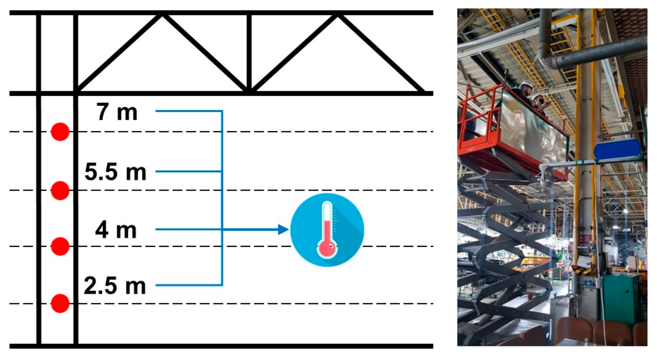
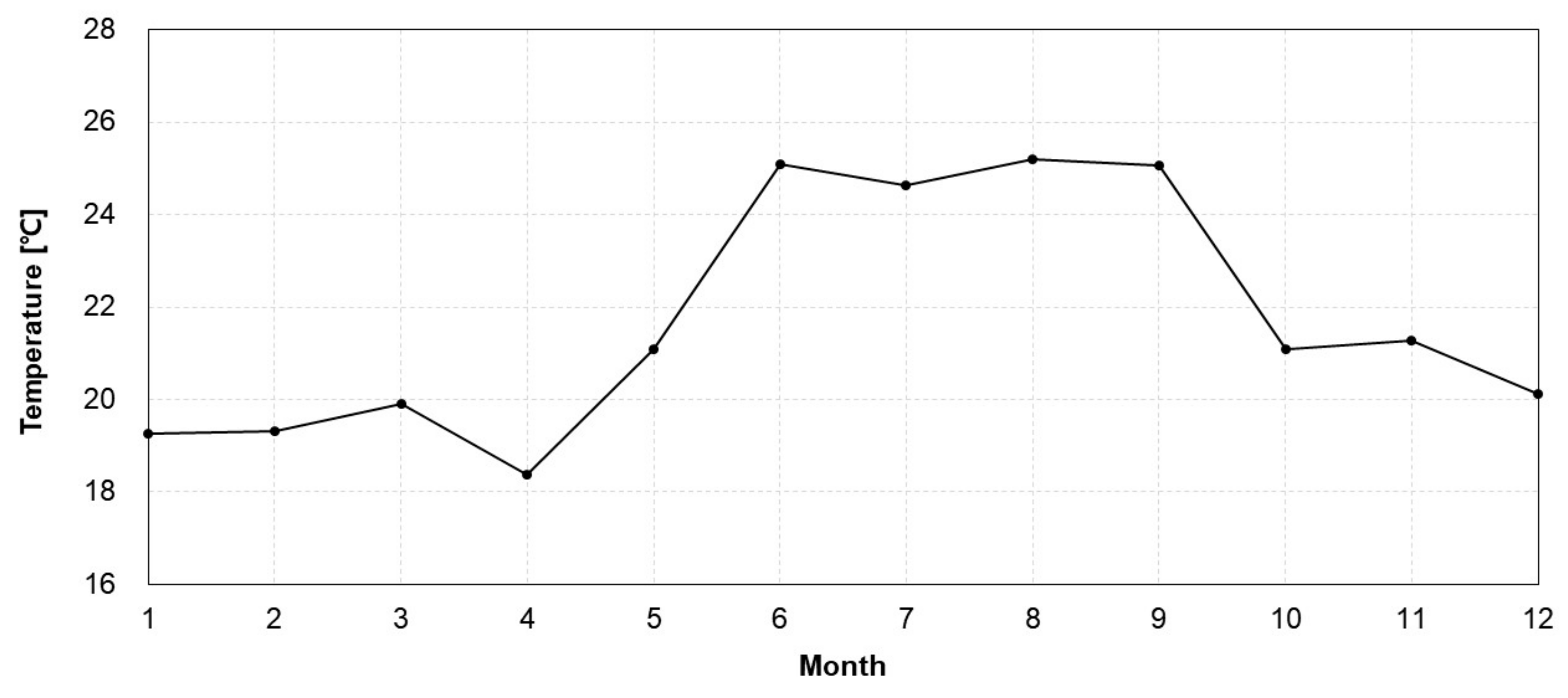
3.1.2. Zone Air Temperature
- Vertical zone air temperature distribution
- 2.
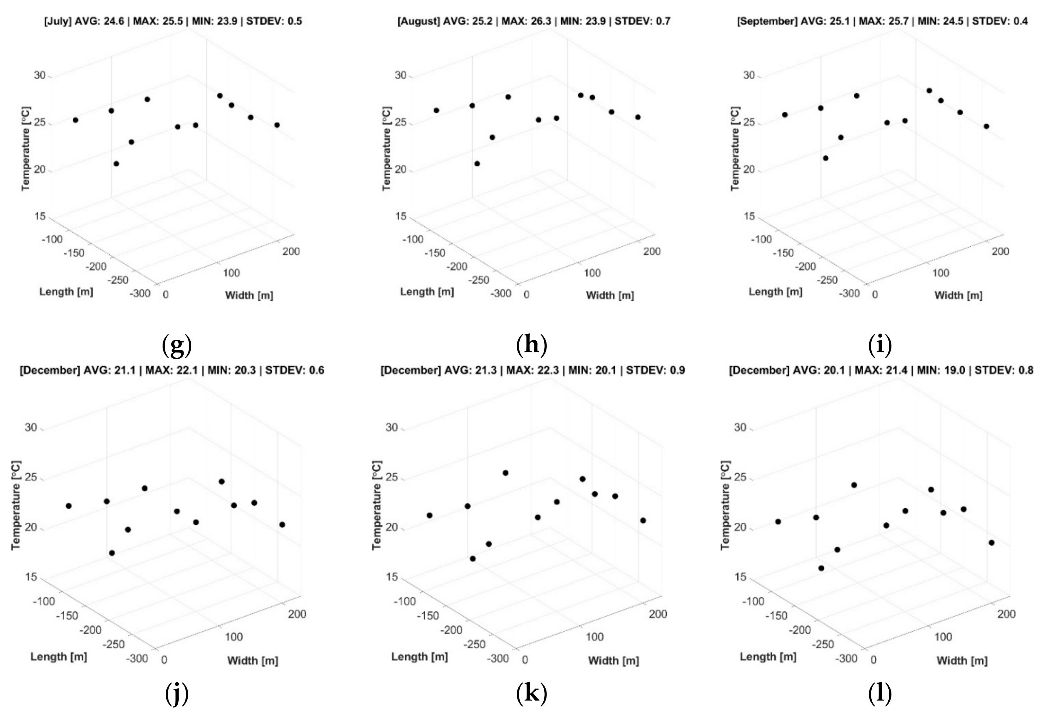
- Horizontal-zone air temperature distribution
3.2. Operation Data-Based Building Profiles
3.2.1. Operation Schedule
3.2.2. Internal Heat Gain
3.2.3. Hot Water Demand
4. Results and Discussion
4.1. Comparison of the Profiles Between the Office and the Factory
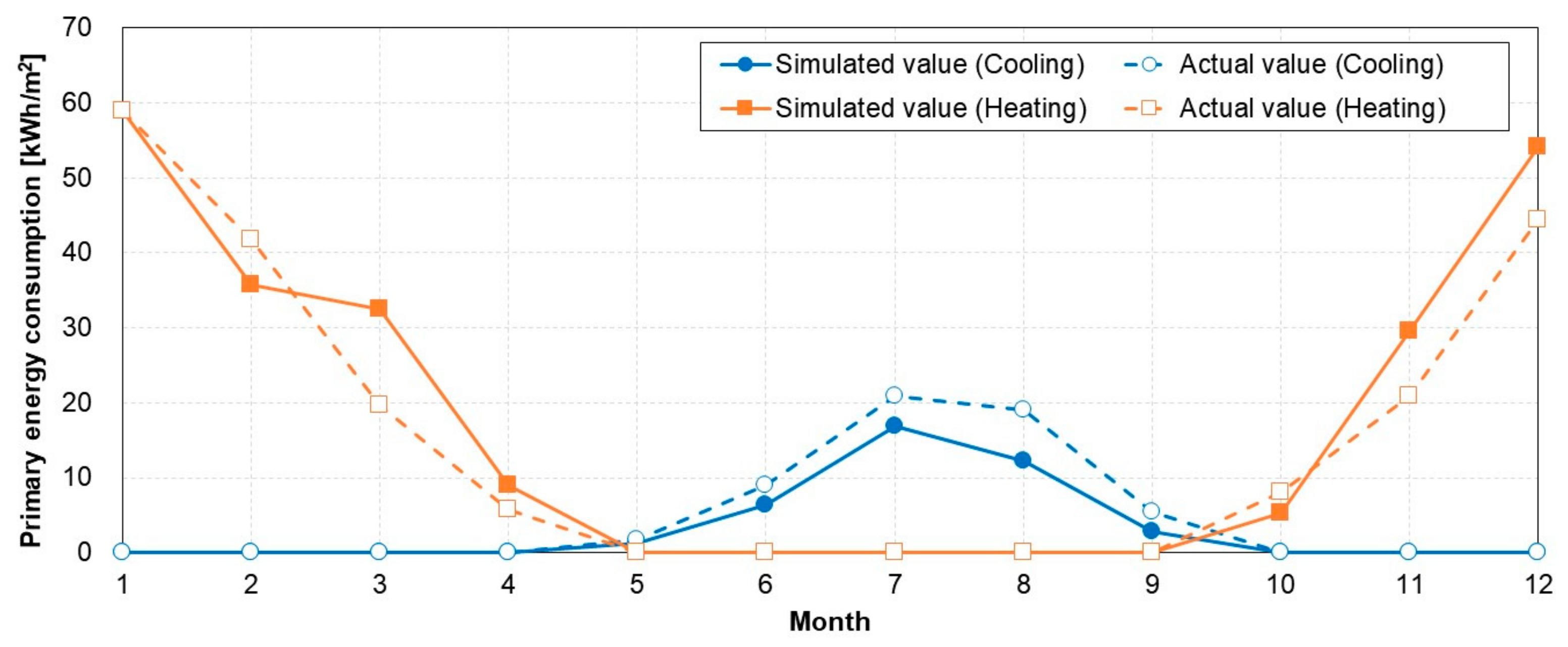
4.2. Energy Simulation Using the Investigated Building Profiles
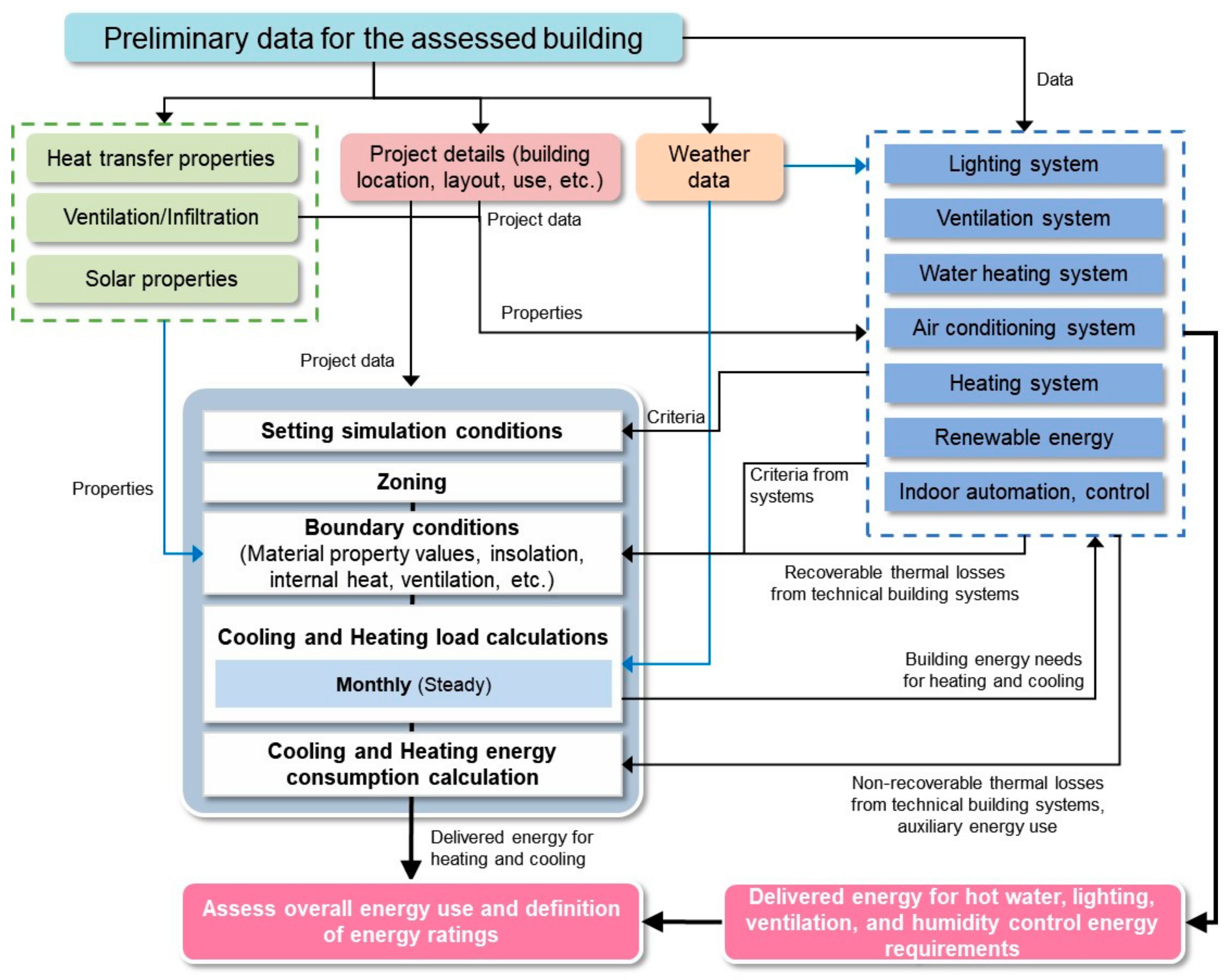
4.2.1. Energy Simulation Method
4.2.2. Performing Simulation and Results
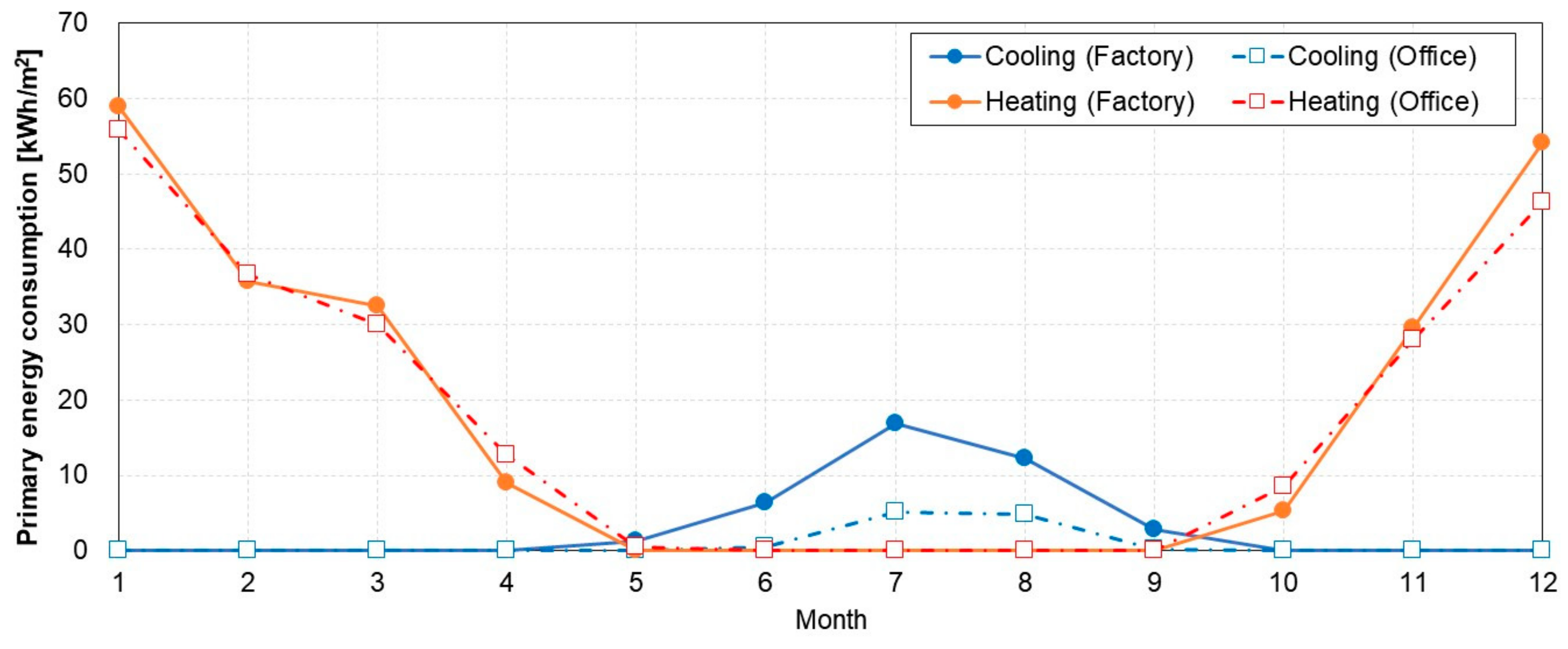
4.3. Energy Simulation of the Factory Based on Office Building Profiles
5. Conclusions
Author Contributions
Funding
Data Availability Statement
Conflicts of Interest
Nomenclature
| A | Total floor area [m2] |
| C | Concentration [PPM] |
| Cp | Specific heat [J/(kg·°C)] |
| G | CO2 generation rate [m3/h] |
| H | Height [m] |
| L | Length [m] |
| n | Number of measurement points [-] |
| N | Number of people [-] |
| p | Measurement point [-] |
| Q | Infiltration rate [m3/h] |
| Qhw | Hot water demand [Wh] |
| t | Time [h] |
| T | Temperature [°C] |
| V | Volume of zone [m3] |
| Vhw | Request amount of hot water [L/(day∙m2)] |
| W | Width [m] |
| Greek Symbols | |
| δC | Room mean square deviation of concentration |
| ω | Humidity ratio [kg/kga] |
| τ | Period [h] |
| Abbreviations | |
| ACH | Air changes per hour [h−1] |
| AHU | Air handling unit |
| Subscript | |
| hw | Hot water |
| OA | Outdoor air |
| RA | Room air |
| tap | Tap water |
| w | Water |
References
- The Government of the Republic of Korea. Fourth Biennial Update Report of the Republic of Korea (Report No. 11-1480906-000005-11). 2021. Available online: https://unfccc.int/documents/418616?gad_source=1&gclid=Cj0KCQiAuou6BhDhARIsAIfgrn4U2AcaaL--0RiMVx_jH9vGTf6XbdQSninrqWTd-HWUl7ROcnZaPv8aAtE6EALw_wcB (accessed on 4 November 2024).
- Tan, Y.; Luo, T.; Xue, X.; Shen, G.Q.; Zhang, G.; Hou, L. An Empirical Study of Green Retrofit Technologies and Policies for Aged Residential Buildings in Hong Kong. J. Build. Eng. 2021, 39, 102271. [Google Scholar] [CrossRef]
- Liu, G.; Tan, Y.; Li, X. China’s Policies of Building Green Retrofit: A State-of-the-Art Overview. Build. Environ. 2020, 169, 106554. [Google Scholar] [CrossRef]
- An, J.; Jung, D.; Jeong, K.; Ji, C.; Hong, T.; Lee, J.; Kapp, S.; Choi, J. Energy-Environmental-Economic Assessment of Green Retrofit Policy to Achieve 2050 Carbon-Neutrality in South Korea: Focused on Residential Buildings. Energy Build. 2023, 289, 113059. [Google Scholar] [CrossRef]
- Moynihan, G.P.; Triantafillu, D. Energy Savings for a Manufacturing Facility Using Building Simulation Modeling: A Case Study. Eng. Manag. J. 2012, 24, 73–84. [Google Scholar] [CrossRef]
- Wright, A.J.; Oates, M.R.; Greenough, R. Concepts for Dynamic Modelling of Energy-Related Flows in Manufacturing. Appl. Energy 2013, 112, 1342–1348. [Google Scholar] [CrossRef]
- Lee, B.; Trcka, M.; Hensen, J.L.M. Building Energy Simulation and Optimization: A Case Study of Industrial Halls with Varying Process Loads and Occupancy Patterns. Build. Simul. 2014, 7, 229–236. [Google Scholar] [CrossRef]
- Gourlis, G.; Kovacic, I. A Study on Building Performance Analysis for Energy Retrofit of Existing Industrial Facilities. Appl. Energy 2016, 184, 1389–1399. [Google Scholar] [CrossRef]
- Gourlis, G.; Kovacic, I. A Holistic Digital Twin Simulation Framework for Industrial Facilities: BIM-Based Data Acquisition for Building Energy Modeling. Front. Built Environ. 2022, 8, 918821. [Google Scholar] [CrossRef]
- Biscione, A.; Felice, A.D.; Gallucci, T. Energy Saving in Transition Economies: Environmental Activities in Manufacturing Firms. Sustainability 2022, 14, 4031. [Google Scholar] [CrossRef]
- Kazakova, E.; Lee, J. Sustainable Manufacturing for a Circular Economy. Sustainability 2022, 14, 17010. [Google Scholar] [CrossRef]
- Tayefeh, A.; Aslani, A.; Zahedi, R.; Yousefi, H. Reducing Energy Consumption in a Factory and Providing an Upgraded Energy System to Improve Energy Performance. Clean. Energy Syst. 2024, 8, 100124. [Google Scholar] [CrossRef]
- Banti, N. Existing Industrial Buildings—A Review on Multidisciplinary Research Trends and Retrofit Solutions. J. Build. Eng. 2024, 84, 108615. [Google Scholar] [CrossRef]
- Katunsky, D.; Korjenic, A.; Katunska, J.; Lopusniak, M.; Korjenic, S.; Doroudiani, S. Analysis of Thermal Energy Demand and Saving in Industrial Buildings: A Case Study in Slovakia. Build. Environ. 2013, 67, 138–146. [Google Scholar] [CrossRef]
- Chowdhury, S.; Shabbir, K.; Hamada, Y. Thermal Performance of Building Envelope of Ready-Made Garments (RMG) Factories in Dhaka, Bangladesh. Energy Build. 2015, 107, 144–154. [Google Scholar] [CrossRef]
- Weeber, M.; Ghisi, E.; Sauer, A. Applying Energy Building Simulation in the Assessment of Energy Efficiency Measures in Factories. Procedia CIRP 2018, 69, 336–341. [Google Scholar] [CrossRef]
- Hesselbach, J.; Herrmann, C.; Detzer, R.; Martin, L.; Thiede, S.; Lüdemann, B. Energy Efficiency through Optimized Coordination of Production and Technical Building Services. In Proceedings of the LCE2008-15th CIRP International Conference on Life Cycle Engineering, Sydney, Australia, 17–19 March 2008; pp. 624–628. [Google Scholar]
- Duflou, J.R.; Sutherland, J.W.; Dornfeld, D.; Herrmann, C.; Jeswiet, J.; Kara, S.; Hauschild, M.; Kellens, K. CIRP Annals—Manufacturing Technology Towards Energy and Resource Efficient Manufacturing: A Processes and Systems Approach. CIRP Ann.—Manuf. Technol. 2012, 61, 587–609. [Google Scholar] [CrossRef]
- Garwood, T.L.; Hughes, B.R.; Oates, M.R.; Connor, D.O. A Review of Energy Simulation Tools for the Manufacturing Sector. Renew. Sustain. Energy Rev. 2018, 81, 895–911. [Google Scholar] [CrossRef]
- ISO 52016-1; Energy Performance of Buildings—Energy Needs for Heating and Cooling, Internal Temperatures and Sensible and Latent Heat Loads—Part 1: Calculation Procedures. ISO: Geneva, Switzerland, 2017.
- ASTM E1827-11(2017); Standard Test Methods for Determining Airtightness of Buildings Using an Orifice Blower Door. ASTM: West Conshohocken, PA, USA, 2017.
- ASTM E741-11(2017); Standard Test Method for Determining Air Change in a Single Zone by Means of a Tracer Gas Dilution. ASTM: West Conshohocken, PA, USA, 2017.
- Park, S.; Choi, P.; Song, D.; Koo, J. Estimation of the Real-Time Infiltration Rate Using a Low Carbon Dioxide Concentration. J. Build. Eng. 2021, 42, 102835. [Google Scholar] [CrossRef]
- Men, C.; Wang, S.; Zou, Z. Experimental Study on Tracer Gas Method for Building Infiltration Rate Measurement. Build. Serv. Eng. Res. Technol. 2020, 41, 745–757. [Google Scholar] [CrossRef]
- Aronhime, S.; Calcagno, C.; Jajamovich, G.H.; Dyvorne, H.A.; Robson, P.; Dieterich, D.; Chatterji, M.; Fiel, M.I.; Rusinek, H.; Taouli, B. DCE-MRI of the Liver: Effect of Linear and Nonlinear Conversions on Hepatic Perfusion Quantification and Reproducibility. J. Magn. Reson. Imaging 2014, 40, 90–98. [Google Scholar] [CrossRef]
- Liu, H.; Shah, S.; Jiang, W. On-Line Outlier Detection and Data Cleaning. Comput. Chem. Eng. 2004, 28, 1635–1647. [Google Scholar] [CrossRef]
- Cui, S.; Cohen, M.; Stabat, P.; Marchio, D. CO2 Tracer Gas Concentration Decay Method for Measuring Air Change Rate. Build. Environ. 2015, 84, 162–169. [Google Scholar] [CrossRef]
- Open Weather Data of South Korea. Available online: https://www.weather.go.kr/w/index.do (accessed on 13 February 2023).
- American Society of Heating, Refrigerating and Air-Conditioning Engineers. Noneresidential Cooling and Heating Load Calculations; American Society of Heating, Refrigerating and Air-Conditioning Engineers: Peachtree Corners, GA, USA, 2013. [Google Scholar]
- Gourlis, G.; Kovacic, I. Passive Measures for Preventing Summer Overheating in Industrial Buildings under Consideration of Varying Manufacturing Process Loads. Energy 2017, 137, 1175–1185. [Google Scholar] [CrossRef]
- National Renewable Energy Laboratory. Domestic Hot Water Assessment Guidelines (Report No. FS-7A20-50118); National Renewable Energy Laboratory: Jefferson County, CO, USA, 2011.
- Korea Energy Agency. Building Energy Efficiency Rating Certification System Operating Regulations; Korea Energy Agency: Yongin-si, Republic of Korea, 2020. [Google Scholar]
- Korea Standard Assosiation. F 2603: Method for Measuring Amount of Room Ventilation (Carbon Dioxide Method); Korea Standard Assosiation: Seoul, Republic of Korea, 2016. [Google Scholar]
- DIN V 18599-1; Energy Efficiency of Buildings—Calculation of the Net, Final and Primary Energy Demand for Heating, Cooling, Ventilation, Domestic Hot Water and Lighting—Part 1: General Balancing Procedures, Terms and Definitions, Zoning and Evaluation. Deutsches Institut Fur Normung: Berlin, Germany, 2016.
- ISO 13790:2008; Energy Performance of Buildings—Calculation of Energy Use for Space Heating and Cooling. ISO: Geneva, Switzerland, 2008.
- DIN V 18599-5; Energy Efficiency of Buildings—Calculation of the Net, Final and Primary Energy Demand for Heating, Cooling, Ventilation, Domestic Hot Water and Lighting—Part 5: Final Energy Demand of Heating Systems. Deutsches Institut Fur Normung: Berlin, Germany, 2016.
- DIN V 18599-3; Energy Efficiency of Buildings—Calculation of the Net, Final and Primary Energy Demand for Heating, Cooling, Ventilation, Domestic Hot Water and Lighting—Part 3: Net Energy Demand for Air Conditioning. Deutsches Institut Fur Normung: Berlin, Germany, 2016.
- DIN V 18599-8; Energy Efficiency of Buildings—Calculation of the Net, Final and Primary Energy Demand for Heating, Cooling, Ventilation, Domestic Hot Water and Lighting—Part 8: Net and Final Energy Demand of Domestic Hot Water Systems. Deutsches Institut Fur Normung: Berlin, Germany, 2016.
- DIN V 18599-4; Energy Efficiency of Buildings—Calculation of the Net, Final and Primary Energy Demand for Heating, Cooling, Ventilation, Domestic Hot Water and Lighting—Part 4: Net and Final Energy Demand for Lighting. Deutsches Institut Fur Normung: Berlin, Germany, 2016.
- Nouri, A.; van Treeck, C.; Frisch, J. Sensitivity Assessment of Building Energy Performance Simulations Using MARS Meta-Modeling in Combination with Sobol’ Method. Energies 2024, 17, 695. [Google Scholar] [CrossRef]
- Sandels, C.; Brodén, D.; Widén, J.; Nordström, L.; Andersson, E. Modeling Office Building Consumer Load with a Combined Physical and Behavioral Approach: Simulation and Validation. Appl. Energy 2016, 162, 472–485. [Google Scholar] [CrossRef]
- Nageler, P.; Schweiger, G.; Pichler, M.; Brandl, D.; Mach, T.; Heimrath, R.; Schranzhofer, H.; Hochenauer, C. Validation of Dynamic Building Energy Simulation Tools Based on a Real Test-Box with Thermally Activated Building Systems (TABS). Energy Build. 2018, 168, 42–55. [Google Scholar] [CrossRef]
- Barone, G.; Buonomano, A.; Forzano, C.; Palombo, A. Building Energy Performance Analysis: An Experimental Validation of an in-House Dynamic Simulation Tool through a Real Test Room. Energies 2019, 12, 4107. [Google Scholar] [CrossRef]


| Start Time | End Time | |
|---|---|---|
| HVAC Schedule | 6:00 am | 1:00 am (+day1) |
| Occupant Schedule | 7:00 am | 0:00 am (+day1) |
| Building Profiles | Factory | Office (>30 m2) | |
|---|---|---|---|
| Operation schedule | Occupant | 7:00–24:00 | 9:00–18:00 |
| HVAC | 6:00–1:00 | 7:00–18:00 | |
| ACH [h−1] | 0.367 | 0.3 | |
| Minimum outdoor air flow rate per area [m3/(h∙m2)] | 5.13 | 6 | |
| Required hot water per area [Wh/(day∙m2)] | 1.47 | 30 | |
| Internal heat gain [Wh/(day∙m2)] | Occupant | 38 | 55.8 |
| Equipment | 414 | 126 | |
| Set point [°C] | Heating | 19.8 | 20 |
| Cooling | 25.0 | 26 | |
| Monthly day of use [days] | January | 24 | 22 |
| February | 20 | 19 | |
| March | 26 | 21 | |
| April | 25 | 22 | |
| May | 23 | 22 | |
| June | 26 | 20 | |
| July | 26 | 22 | |
| August | 19 | 21 | |
| September | 20 | 18 | |
| October | 26 | 21 | |
| November | 26 | 21 | |
| December | 26 | 21 | |
| Component | Materials | U-Value [W/m2·K] | G-Value |
|---|---|---|---|
| External wall with insulation |  | 0.48 | – |
| External wall without insulation |  | 2.40 | – |
| Floor |  | 3.16 | – |
| Roof | 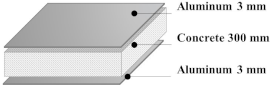 | 0.50 | – |
| Single-glazed window |  | 6.60 | 0.688 |
| Door | 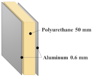 | 0.48 | – |
Disclaimer/Publisher’s Note: The statements, opinions and data contained in all publications are solely those of the individual author(s) and contributor(s) and not of MDPI and/or the editor(s). MDPI and/or the editor(s) disclaim responsibility for any injury to people or property resulting from any ideas, methods, instructions or products referred to in the content. |
© 2024 by the authors. Licensee MDPI, Basel, Switzerland. This article is an open access article distributed under the terms and conditions of the Creative Commons Attribution (CC BY) license (https://creativecommons.org/licenses/by/4.0/).
Share and Cite
Lim, H.; Park, G.-H.; Kim, S.; Kim, Y.; Yu, K.-H. Investigation of Building Profiles for the Energy Simulation of a Factory Building: A Case Study in South Korea. Buildings 2024, 14, 3767. https://doi.org/10.3390/buildings14123767
Lim H, Park G-H, Kim S, Kim Y, Yu K-H. Investigation of Building Profiles for the Energy Simulation of a Factory Building: A Case Study in South Korea. Buildings. 2024; 14(12):3767. https://doi.org/10.3390/buildings14123767
Chicago/Turabian StyleLim, Hansol, Guan-Ho Park, Seheon Kim, Yeweon Kim, and Ki-Hyung Yu. 2024. "Investigation of Building Profiles for the Energy Simulation of a Factory Building: A Case Study in South Korea" Buildings 14, no. 12: 3767. https://doi.org/10.3390/buildings14123767
APA StyleLim, H., Park, G.-H., Kim, S., Kim, Y., & Yu, K.-H. (2024). Investigation of Building Profiles for the Energy Simulation of a Factory Building: A Case Study in South Korea. Buildings, 14(12), 3767. https://doi.org/10.3390/buildings14123767