Optimal Cost Design of RC T-Shaped Combined Footings

Abstract

This paper shows the optimal cost design for T-shaped combined footings of reinforced concrete (RC), which are subjected to biaxial bending in each column to determine the steel areas and the thickness of the footings assuming a linear distribution of soil pressure. The methodology used in this paper is as follows: First, the minimum contact surface between the footing and the ground is investigated. The design equations for the combined footing are then used to determine the objective function and its constraints to obtain the lowest cost, taking into account the ACI code requirements. Flowcharts are shown for the lowest cost and the use of Maple 15 software. The current model for design is developed as follows: A footing thickness is proposed, and then it is verified that the thickness complies with the effects produced by moments, bending shears, and punching shears. Furthermore, four numerical examples are presented under the same loads and moments applied to each column, with different conditions applied to obtain the optimal contact surface and then the minimum cost design. The results show that the optimal cost design (lowest cost) is more economical and more accurate than any other model, and there is no direct proportion between the minimum contact surface and lowest cost for the design of T-shaped combined footings. In this way, the minimum cost model shown in this work can be applied to the design of rectangular and T-shaped combined footings using optimization techniques.

1. Introduction

Optimization is based on mathematically modeling the main characteristics that define the qualities of engineering problems and then, using an algorithm or mathematical model and with the help of a computer, finding the optimal solution.

Mathematical models for structure foundations have aroused great interest among researchers. The main contributions to the optimal design of RC foundations are as follows: Vrecl-Kojc presented an optimization method for anchored pile walls and the impacts of several parameters on costs using a nonlinear programming approach [1]. Wang and Kulhawy studied a design including construction economics, and their results presented foundations with minimal construction costs [2]. Kortnik optimized the planning procedure for high-security pillars for subterranean excavation of natural rock blocks [3]. Wang investigated a design perspective that includes economic design optimization with reliable methodologies developed to act rationally in the face of geotechnically related uncertainties [4]. Chagoyén et al. estimated the optimal design for foundations considering the minimum cost criterion [5]. Basudhar et al. proposed an optimal cost for a circular footing under generalized loads using the unconstrained sequential minimization technique together with Powell’s conjugate direction method [6]. Rizwan et al. presented a computational procedure to find the optimal cost design for RC combined footings (minimum cost); the software they used is based on the application of the Visual Basics Net programming language to develop the structural analysis, design, and optimization of the combined footings [7]. Jagodnik et al. reviewed the deformation of a Winkler’s soil-supported beam using Bernoulli theory via the mixed finite element method [8]. Al-Ansari formulated a model to estimate the optimal cost design for RC isolated footings by applying the design constraints of the ACI building code [9]. Jelusic and Zlender estimated an optimized model to obtain the safety factors of walls with different inclinations, the terrain slope angle, the length of the nails, and the diameter of the bore [10]. Al-Ansari presented an analysis and optimal cost design for casing footings with different proportions according to the ACI design code to minimize the cost of a foundation [11]. Sadoğlu studied an optimization problem on symmetrical gravity retaining walls of different heights for continuous functions [12]. El-Sakhawy et al. presented different foundation shapes that resemble the distribution of footing stresses on the underlying soft soils to minimize their effect; they used elliptical, trapezoidal, and inverted folded foundations as alternatives to conventional shallow flat footings [13]. Ukritchon and Keawsawasvong presented a practical method to optimize the design of a continuous footing under vertical and horizontal loads; their design problem, which was to estimate the optimal dimension of the footing and the minimum amount of reinforcing steel required, was formulated in a nonlinear minimization form [14]. Velázquez-Santillán et al. estimated an optimal cost design for RC rectangular combined footings [15]. Luévanos-Rojas et al. formulated a model to obtain the minimum dimensions and the equations for design of RC T-shaped combined footings [16,17]. Nigdeli et al. presented a methodology based on the cost optimization of RC footings by employing several classical algorithms recently developed to address non-linear optimization problems [18]. Islam and Rokonuzzaman developed an optimized foundation design process using genetic algorithms; the objective function of these algorithms is the reduction of construction costs, which include design parameters and design requirements such as optimization variables and constraints [19]. Using Excel, Rawat and Mittal studied a solution-based model which aims to provide a procedure that reduces construction costs by simultaneously integrating design parameters and requirements as optimization variables and constraints, respectively [20]. Chaudhuri and Maity estimated the optimal cost for an isolated foundation as per Indian Standard (IS) Code 456:2000 [21]. Nawaz et al. used a generalized reduced gradient method for the optimal cost design of isolated footings in cohesive soils [22]. Waheed et al. presented a parametric study using a practical metaheuristic tool for the optimal cost design of RC isolated footings [23]. Nigdeli and Bekdas investigated the orientation of a column located eccentrically with respect to the center of the footing in an optimal design [24]. Kashani et al. estimated the optimal cost design for combined footings using five swarm intelligence algorithms: particle swarm optimization (PSO), accelerated particle swarm optimization (APSO), whale optimization algorithm (WOA), ant lion optimizer (ALO), and moth flame optimization (MFO) [25]. Aishwarya and Balaji analyzed and designed a corner combined footing for eccentrically loaded rectangular columns which transfers the center of gravity of the loads to the center of gravity of the footing [26]. López-Machado et al. performed a comparison of the structural designs of two six-story RC buildings considering the soil–structure interaction [27]. Komolafe et al. studied square and circular footings resting on non-cohesive soils from geotechnical, structural, and construction cost perspectives [28]. Ekbote and Nainegali investigated asymmetrical close-spaced footings supported on reinforced soil [29]. Solorzano and Plevris formulated an optimal cost design for rectangular footings using genetic algorithms according to the American Concrete Institute (AC() design code [30]. Chaabani et al. analyzed the ultimate bearing capacity of continuous footings on a reinforced sand layer over clay with voids [31]. Gnananandarao et al. performed several loading tests of a T-shaped skirted footing by varying the skirt depth and the relative sand density [32]. Shaaban et al. investigated a general equation to determine the maximum pressure at the base of a trapezoidal and triangular footing under biaxial bending [33]. Al-Ansari and Afzal investigated a simplified analysis for the design of square, triangular, circular and trapezoidal reinforced concrete footings supporting a square column under biaxial bending [34]. Ranadive and Mahiyar experimentally studied several tests of T-shaped footings subjected to dynamic loading [35]. Khare and Thakare determined the ultimate bearing capacity of T-shaped footings assuming that the soil beneath the foundations is homogeneous [36]. Sivanantham et al. determined the influence of the filling in an RC frame supported on slopes subjected to lateral loads [37]. Helis et al. obtained the bearing capacity of circular footings rested on sandy soils using two reinforcement systems, the grid and the geogrid anchor [38].

After reviewing of the literature, there were two works closest to the topic of T-shaped combined: Luévanos-Rojas et al. developed a model to estimate the smallest contact area with the ground and the dimensions of the footing [16]. Luévanos-Rojas et al. presented the equations for the design of RC T-shaped combined footings [17]. These works do not show the complete minimum cost design. That is, only the equations for the design are presented, and the methodology by integration is presented to then determine the integration constant. The solved examples are obtained by trial and error, and this does not guarantee that it is the minimum cost design. Therefore, there are no works on the subject with the current knowledge on structural design to optimize RC T-shaped combined footings.

This paper presents the optimal cost design of RC T-shaped combined footings under biaxial bending at each column to obtain the thicknesses and steel areas of the footings. This paper shows the objective function and constraint functions for the design of T-shaped combined footings. The current design model is developed as follows: the thickness of the footings is proposed, and then it is verified that the thickness complies with the effects produced by moments, bending shears and punching shears. In addition, four numerical examples are presented under the same loads and moments applied on each column with different conditions to obtain the optimal contact surface and then the optimal cost design of RC T-shaped combined footings to observe the accuracy of the optimal model shown in this paper.

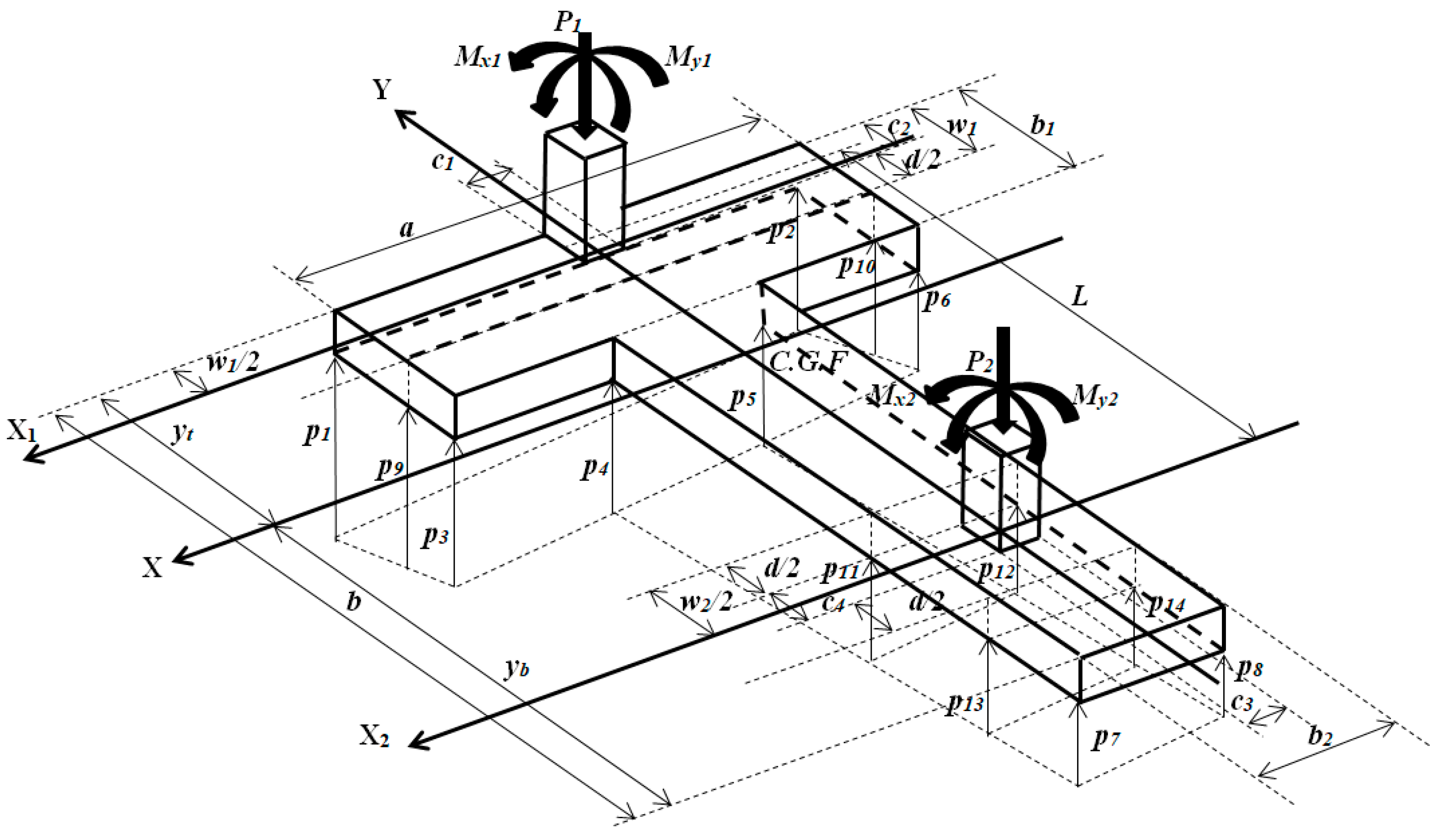
2. Mathematical Models

The p_aa (available allowable ground pressure) is estimated by the following equation [16,17]:

$$p_{aa}=p_a-{\gamma }_{wf}-{\gamma }_{ws},$$

(1)

$$p_{aa}=p_a-{\gamma }_{cd}\left(d+r\right)-{\gamma }_{sd}\left(H-d-r\right),$$

(2)

where: p_a = allowable ground pressure (kN/m²), γ_wf = footing weight (kN/m²), γ_ws = weight of soil fill (kN/m²), γ_sd = soil density (kN/m³), γ_cd = concrete density = 24 kN/m³, H = depth of the foundation measured from the base of the foundation to the free surface of the soil (m), r = coating of the foundation (m), d = effective depth of foundation (m).

If the load combinations include earthquake and/or wind, the allowable soil pressure should be increased by 33% [39].

Figure 1 shows a T-shaped combined footing supporting two rectangular columns of various dimensions (one interior column and one boundary column) under biaxial bending (two-way bending) at each column.

Table 1. Coordinates of the pressures on the footing for longitudinal analysis.

Pressures pn (kN/m2)	p1	p2	p3	p4	p5	p6	p7	p8
Coordinates	x1 = a/2	x2 = −a/2	x3 = a/2	x4 = b2/2	x5 = −b2/2	x6 = −a/2	x7 = b2/2	x8 = −b2/2
	y1 = yt	y2 = yt	y3 = yt − b1	y4 = yt − b1	y5 = yt − b1	y6 = yt − b1	y7 = −yb	y8 = −yb

presents the pressure coordinates at each vertex of the footing (X and Y axes).

Table 2. Coordinates of the pressures on the footing for the cross-sectional analysis.

Pressures pn (kN/m2)	Pressures Due to P1 pn (kN/m2)				Pressures Due to P2 pn (kN/m2)
	p1	p2	p9	p10	p11	p12	p13	p14
Coordinates	x1 = a/2	x2 = −a/2	x9 = a/2	x10 = −a/2	x11 = b2/2	x12 = −b2/2	x13 = b2/2	x14 = −b2/2
	y1 = w1/2	y2 = w1/2	y9 = −w1/2	y10 = −w1/2	y11 = w2/2	y12 = w2/2	y13 = −w2/2	y14 = −w2/2

shows the coordinates of the pressures at each vertex of the footing due to column 1 (X₁ and Y₁ axes), and the coordinates of the pressures at each vertex of the footing due to column 2 (X₂ and Y₂ axes).

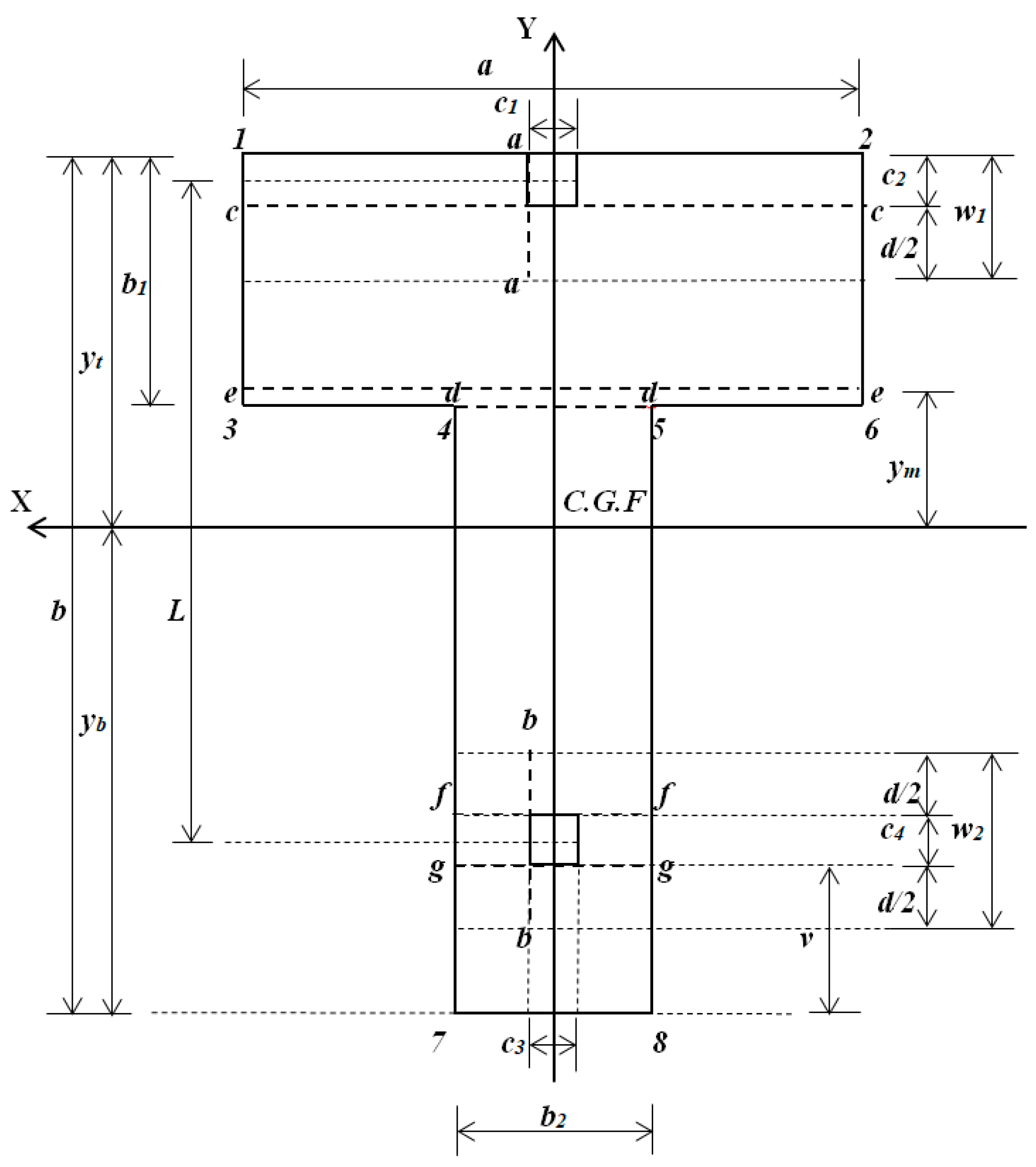
2.1. Minimum Contact Surface

In this subsection, it is assumed that the ground contact area works completely under compression to determine the smallest area.

The objective function to determine the minimum contact surface with the ground “S_min” is as follows [16]:

$$S_{min}=\left(a-b_2\right)b_1+b{b}_2.$$

(3)

The constraint functions are

$$p_n={\displaystyle \frac{R}{S}}+{\displaystyle \frac{M_{xT}{y}_n}{I_x}}+{\displaystyle \frac{M_{yT}{x}_n}{2I_y}},$$

(4)

$$R=P_1+P_2,$$

(5)

$$M_{xT}=M_{x1}+M_{x2}+R\left(y_t-{\displaystyle \frac{c_2}{2}}\right)-P_{2}L,$$

(6)

$$M_{yT}=M_{y1}+M_{y2},$$

(7)

$$y_t={\displaystyle \frac{\left(a-b_2\right){b_1}^2+b^2{b}_2}{2S}},$$

(8)

$$y_b={\displaystyle \frac{\left(2b-b_1\right)\left(a-b_2\right)b_1+b^2{b}_2}{2S}},$$

(9)

$$I_x={\displaystyle \frac{a^2{b_1}^4+2a{b}_1{b}_2\left(b-b_1\right)\left(2b^2-b{b}_1+{b_1}^2\right)+{b_2}^2{\left(b-b_1\right)}^4}{12S}},$$

(10)

$$I_y={\displaystyle \frac{b_1{a}^3+\left(b-b_1\right){b_2}^3}{12}},$$

(11)

$$0\le \left\{\begin{array}{c}{p}_1\\ p_2\\ \begin{array}{c}{p}_3\\ p_4\\ \begin{array}{c}\begin{array}{c}\begin{array}{c}{p}_5\\ p_6\end{array}\\ p_7\end{array}\\ p_8\end{array}\end{array}\end{array}\right\}\le p_{aa},$$

(12)

$${\displaystyle \frac{c_2}{2}}+L+{\displaystyle \frac{c_4}{2}}\le b,$$

(13)

where R = resultant force (kN); M_xT and M_yT = resultant moments about the X and Y axes (kN-m); x_n and y_n = coordinates of the point under study (m); I_x and I_y = moments of inertia about the X and Y axes (m⁴).

2.2. Minimum Cost Design

In this subsection, it is assumed that the contact area on the soil is known (Section 2.1) to obtain the lowest design cost due to the moments, bending shears and punching shears acting on the footing.

The factored soil pressures anywhere on the contact surface of the footing due to the factored load and the factored moments for the T-shaped combined footing are obtained as shown below.

The pressure in the main direction (Y axis) is

$$p_u\left(x,y\right)={\displaystyle \frac{R_u}{S}}+{\displaystyle \frac{M_{uxT}y}{I_x}}+{\displaystyle \frac{M_{uyT}x}{I_y}},$$

(14)

where R_u = factored resultant force, M_uxT and M_uyT = factored resultant moments in two directions (X and Y).

The pressure in the transverse direction to the main direction (X₁ axis) is

$$p_{{uP}_1}\left(x_1,y_1\right)={\displaystyle \frac{P_{u1}}{w_{1}a}}+{\displaystyle \frac{12\left[M_{ux1}+P_{u1}\left(w_1-c_2\right)/2\right]y}{{w_1}^{3}a}}+{\displaystyle \frac{12M_{uy1}x}{w_1{a}^3}},$$

(15)

where w₁ = width of analysis surface for column 1 of w₁ = c₂ + d/2, P_u1 = factored axial load in column 1, M_ux1 = factored moment in X₁ axis of column 1, M_uy1 = factored moment in Y₁ axis of column 1.

The pressure in the transverse direction to the main direction (X₂ axis) is

$$p_{{uP}_2}\left(x_2,y_2\right)={\displaystyle \frac{P_{u2}}{w_2{b}_2}}+{\displaystyle \frac{12\left[M_{ux2}+P_{u2}\left(w_2-c_4\right)/2\right]y}{{w_2}^3{b}_2}}+{\displaystyle \frac{12M_{uy2}x}{w_2{b_2}^3}},$$

(16)

where w₂ = width of analysis surface for column 2 in the transverse direction of w₂ = c₄ + d/2 + v (if d/2 ≤ v → v = d/2, and if d/2 ≥ v → v = b − L − (c₂ + c₄)/2), P_u2 = factored axial load in column 2, M_ux2 = factored moment in X₂ axis of column 2, M_uy2 = factored moment in Y₂ axis of column 2.

2.2.1. Moments

The factored moments according to the ACI code are shown on the axes: a, b, c, d, e, f and g (see Figure 2).

The factored moments applied to the footing on axes a and b (axes parallel to the Y axis) are obtained:

$$M_{ua}=-{\int }_{-{\displaystyle \frac{w_1}{2}}}^{{\displaystyle \frac{w_1}{2}}}{\int }_{{\displaystyle \frac{c_1}{2}}}^{{\displaystyle \frac{a}{2}}}{p}_{{uP}_1}\left(x_1,y_1\right)\left(x-{\displaystyle \frac{c_1}{2}}\right)dxdy,$$

(17)

$$M_{ua}=-{\displaystyle \frac{P_{u1}{\left(a-c_1\right)}^2}{8a}}-{\displaystyle \frac{M_{uy1}\left(2a+c_1\right){\left(a-c_1\right)}^2}{4a^3}},$$

(18)

$$M_{ub}=-{\int }_{-{\displaystyle \frac{w_2}{2}}}^{{\displaystyle \frac{w_2}{2}}}{\int }_{{\displaystyle \frac{c_3}{2}}}^{{\displaystyle \frac{b_2}{2}}}{p}_{{uP}_2}\left(x_2,y_2\right)\left(x-{\displaystyle \frac{c_3}{2}}\right)dxdy,$$

(19)

$$M_{ub}=-{\displaystyle \frac{P_{u2}{\left(b_2-c_3\right)}^2}{8b_2}}-{\displaystyle \frac{M_{uy2}\left(2b_2+c_3\right){\left(b_2-c_3\right)}^2}{4{b_2}^3}}.$$

(20)

The factored moments acting on the footing on the axes c, d, e, f and g (axes parallel to the X axis) are obtained:

$$M_{uc}={\displaystyle \frac{P_{u1}{c}_2}{2}}+M_{ux1}-{\int }_{y_t-c_2}^{y_t}{\int }_{-{\displaystyle \frac{a}{2}}}^{{\displaystyle \frac{a}{2}}}{p}_u\left(x,y\right)\left(y-y_t+c_2\right)dxdy,$$

(21)

$$M_{ud}=P_{u1}\left(b_1-{\displaystyle \frac{c_2}{2}}\right)+M_{ux1}-{\int }_{y_t-b_1}^{y_t}{\int }_{-{\displaystyle \frac{a}{2}}}^{{\displaystyle \frac{a}{2}}}{p}_u\left(x,y\right)\left(y-y_t+b_1\right)dxdy.$$

(22)

If the maximum positive moment M_ue is located in the interval y_t − c₂/2 ≥ y_m ≥ y_t − b₁:

$$M_{ue}=P_{u1}\left(y_t-y_m-{\displaystyle \frac{c_2}{2}}\right)+M_{ux1}-{\int }_{y_m}^{y_t}{\int }_{-{\displaystyle \frac{a}{2}}}^{{\displaystyle \frac{a}{2}}}{p}_u\left(x,y\right)\left(y-y_m\right)dxdy,$$

(23)

If the maximum positive moment M_ue is located in the interval y_t − b₁ ≥ y_m ≥ y_t − L − c₂/2:

$$M_{ue}=P_{u1}\left(y_t-y_m-b_1\right)+M_{ux1}-{\int }_{y_t-b_1}^{y_t}{\int }_{-{\displaystyle \frac{a}{2}}}^{{\displaystyle \frac{a}{2}}}{p}_u\left(x,y\right)\left(y-y_m\right)dxdy-{\int }_{y_m}^{y_t-b_1}{\int }_{-{\displaystyle \frac{b_2}{2}}}^{{\displaystyle \frac{b_2}{2}}}{p}_u\left(x,y\right)\left(y-y_m\right)dxdy,$$

(24)

$$\begin{gathered} M_{uf}=P_{u1}\left(L-{\displaystyle \frac{c_4}{2}}\right)+M_{ux1}-{\int }_{y_t-b_1}^{y_t}{\int }_{-{\displaystyle \frac{a}{2}}}^{{\displaystyle \frac{a}{2}}}{p}_u\left(x,y\right)\left(y-y_t+L+{\displaystyle \frac{c_2}{2}}-{\displaystyle \frac{c_4}{2}}\right)dxdy \\ -{\int }_{y_t-L-{\displaystyle \frac{c_2}{2}}+{\displaystyle \frac{c_4}{2}}}^{y_t-b_1}{\int }_{-{\displaystyle \frac{b_2}{2}}}^{{\displaystyle \frac{b_2}{2}}}{p}_u\left(x,y\right)\left(y-y_t+L+{\displaystyle \frac{c_2}{2}}-{\displaystyle \frac{c_4}{2}}\right)dxdy, \end{gathered}$$

(25)

$$\begin{gathered} M_{ug}=P_{u1}\left(L+{\displaystyle \frac{c_4}{2}}\right)+{\displaystyle \frac{P_{u2}{c}_4}{2}}+M_{ux1}+M_{ux2}-{\int }_{y_t-b_1}^{y_t}{\int }_{-{\displaystyle \frac{a}{2}}}^{{\displaystyle \frac{a}{2}}}{p}_u\left(x,y\right)\left(y-y_t+L+{\displaystyle \frac{c_2}{2}}+{\displaystyle \frac{c_4}{2}}\right)dxdy \\ -{\int }_{y_t-L-{\displaystyle \frac{c_2}{2}}-{\displaystyle \frac{c_4}{2}}}^{y_t-b_1}{\int }_{-{\displaystyle \frac{b_2}{2}}}^{{\displaystyle \frac{b_2}{2}}}{p}_u\left(x,y\right)\left(y-y_t+L+{\displaystyle \frac{c_2}{2}}+{\displaystyle \frac{c_4}{2}}\right)dxdy \end{gathered}$$

(26)

The positive maximum moment M_ue is obtained as follows: Case (1) Equation (23) is derived, and this equation is set equal to zero to find the position of the maximum moment y_m (if it falls within the interval y_t − c₂/2 ≥ y_m ≥ y_t − b₁), and then substituted into Equation (23); Case (2) Equation (24) is derived, and this equation is set equal to zero to find the position of the maximum moment y_m (if it falls within the interval y_t − b₁ ≥ y_m ≥ y_t − L − c₂/2), and then substituted into Equation (24).

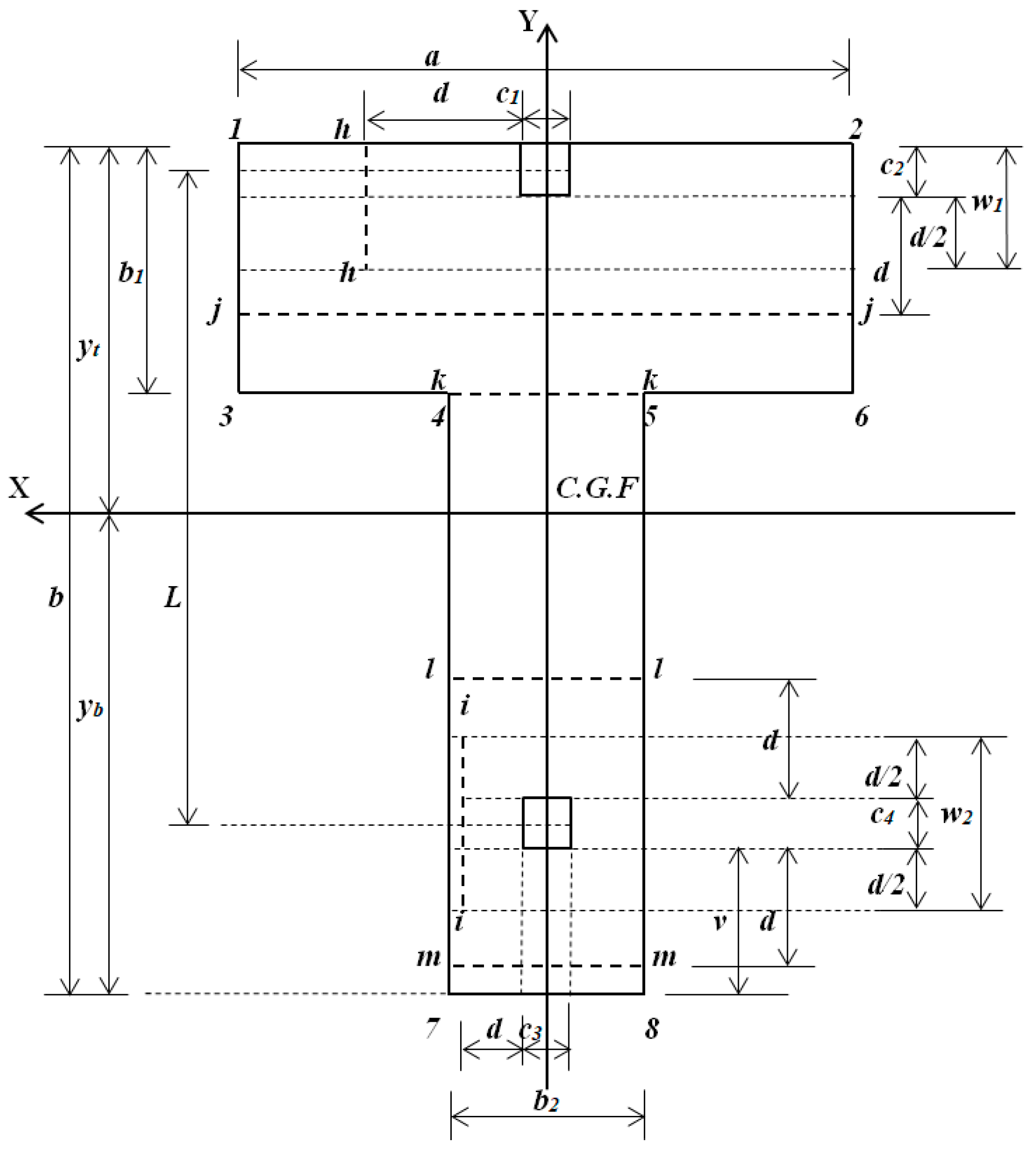
2.2.2. Bending Shears

The factored bending shears according to the ACI code are presented on the axes: h, i, j, k, l and m (see Figure 3).

The factored bending shears applied to the footing in the h and i axes (axes parallel to the Y axis) are obtained:

$$V_{ufh}=-{\int }_{-{\displaystyle \frac{w_1}{2}}}^{{\displaystyle \frac{w_1}{2}}}{\int }_{{\displaystyle \frac{c_1}{2}}+d}^{{\displaystyle \frac{a}{2}}}{p}_{{uP}_1}\left(x_1,y_1\right)dxdy,$$

(27)

$$V_{ufh}=-{\displaystyle \frac{P_{u1}\left(a-c_1-2d\right)}{2a}}-{\displaystyle \frac{3M_{uy1}\left[a^2-{\left(c_1+2d\right)}^2\right]}{2a^3}},$$

(28)

$$V_{ufi}=-{\int }_{-{\displaystyle \frac{w_2}{2}}}^{{\displaystyle \frac{w_2}{2}}}{\int }_{{\displaystyle \frac{c_3}{2}}+d}^{{\displaystyle \frac{b_2}{2}}}{p}_{{uP}_2}\left(x_2,y_2\right)dxdy,$$

(29)

$$V_{ufi}=-{\displaystyle \frac{P_{u2}\left(b_2-c_3-2d\right)}{2b_2}}-{\displaystyle \frac{3M_{uy2}\left[{b_2}^2-{\left(c_3+2d\right)}^2\right]}{2{b_2}^3}}.$$

(30)

where d = effective depth of the footing.

The factored bending shears applied to the footing on the j, k, l and m axes (axes parallel to the X axis) are obtained:

$$V_{ufj}=P_{u1}-{\int }_{y_t-c_2-d}^{y_t}{\int }_{-{\displaystyle \frac{a}{2}}}^{{\displaystyle \frac{a}{2}}}{p}_u\left(x,y\right)dxdy,$$

(31)

$$V_{ufk}=P_{u1}-{\int }_{y_t-b_1}^{y_t}{\int }_{-{\displaystyle \frac{a}{2}}}^{{\displaystyle \frac{a}{2}}}{p}_u\left(x,y\right)dxdy,$$

(32)

$$V_{ufl}=P_{u1}-{\int }_{y_t-b_1}^{y_t}{\int }_{-{\displaystyle \frac{a}{2}}}^{{\displaystyle \frac{a}{2}}}{p}_u\left(x,y\right)dxdy-{\int }_{y_t-L-{\displaystyle \frac{c_2}{2}}+{\displaystyle \frac{c_4}{2}}+d}^{y_t-b_1}{\int }_{-{\displaystyle \frac{b_2}{2}}}^{{\displaystyle \frac{b_2}{2}}}{p}_u\left(x,y\right)dxdy,$$

(33)

$$V_{ufm}=P_{u1}-{\int }_{y_t-b_1}^{y_t}{\int }_{-{\displaystyle \frac{a}{2}}}^{{\displaystyle \frac{a}{2}}}{p}_u\left(x,y\right)dxdy-{\int }_{y_t-L-{\displaystyle \frac{c_2}{2}}-{\displaystyle \frac{c_4}{2}}-d}^{y_t-b_1}{\int }_{-{\displaystyle \frac{b_2}{2}}}^{{\displaystyle \frac{b_2}{2}}}{p}_u\left(x,y\right)dxdy,$$

(34)

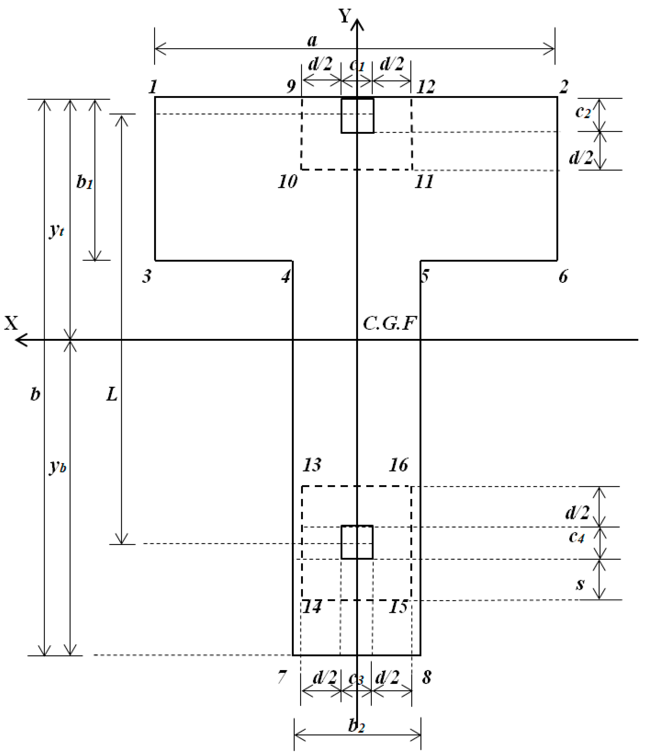
2.2.3. Punching Shears

The factored punching shears according to the ACI code are presented on the perimeter formed by points 9, 10, 11 and 12 for column 1 (boundary column), and by points 13, 14, 15 and 16 for column 2 (interior column) (see Figure 4).

The factored punching shears applied to the footing due to each column are obtained:

$$V_{up1}=P_{u1}-{\int }_{y_t-c_2-{\displaystyle \frac{d}{2}}}^{y_t}{\int }_{-{\displaystyle \frac{c_1}{2}}-{\displaystyle \frac{d}{2}}}^{{\displaystyle \frac{c_1}{2}}+{\displaystyle \frac{d}{2}}}{p}_u\left(x,y\right)dxdy,$$

(35)

$$V_{up2}=P_{u2}-{\int }_{y_t-L-{\displaystyle \frac{c_2}{2}}--{\displaystyle \frac{c_4}{2}}-s}^{y_t-L-{\displaystyle \frac{c_2}{2}}+{\displaystyle \frac{c_4}{2}}+{\displaystyle \frac{d}{2}}}{\int }_{-{\displaystyle \frac{c_3}{2}}-{\displaystyle \frac{d}{2}}}^{{\displaystyle \frac{c_3}{2}}+{\displaystyle \frac{d}{2}}}{p}_u\left(x,y\right)dxdy,$$

(36)

where s must satisfy the following relationships: if d/2 ≤ b − L − c₂/2 − c₄/2 → s = d/2, and if d/2 ≥ b − L − c₂/2 − c₄/2 → s = b − L − c₂/2 − c₄/2.

2.2.4. Objective Function for Minimum Cost

The minimum cost of the T-shaped combined footing is

$$C_{min}=V_c{C}_c+{V_s\gamma }_s{C}_s,$$

(37)

where C_min = minimum cost (dollars), V_c = volume of concrete (m³), C_c = cost of concrete including materials and labor (dollars/m³), V_s = volume of steel (m³), C_s = cost of steel (dollars/kN), γ_s = density of steel = 76.94 kN/m³, C_s = cost of steel (dollars/kN).

The volumes for the T-shaped combined footings are

$$V_s=\left(A_{syTb}+A_{syBb}\right)b+\left(A_{syT{b}_1}+A_{syB{b}_1}\right)b_1+\left(A_{sxTa}+A_{s{P}_{1}a}+A_{sxBa}\right)a+\left(A_{sxT{b}_2}+A_{s{P}_2{b}_2}+A_{sxB{b}_2}\right)b_2,$$

(38)

$$\begin{gathered} V_c=\left[\left(a-b_2\right)b_1+b{b}_2\right]t-\left(A_{syTb}+A_{syBb}\right)b-\left(A_{syT{b}_1}+A_{syB{b}_1}\right)b_1-\left(A_{sxTa}+A_{s{P}_{1}a}+A_{sxBa}\right)a \\ -\left(A_{sxT{b}_2}+A_{s{P}_2{b}_2}+A_{sxB{b}_2}\right)b_2, \end{gathered}$$

(39)

where t = total thickness of the footing (m), A_syTb = steel area at the top with width b₂ (Y-axis direction) (m²), A_syBb = steel area at the bottom with width b₂ (Y-axis direction) (m²), A_syTb1 = steel area at the top with a width (a − b₂) which is the excess part of width b₂ (Y-axis direction) (m²), A_syBb1 = steel area at the bottom with a width (a − b₂) which is the excess part of width b₂ (Y-axis direction) (m²), A_sxTa = steel area at the top with width b₁ (X-axis direction) (m²), A_sP1a = steel area at the bottom under column 1 with width w₁ (X-axis direction) (m²), A_sxBa = steel area in the X-axis direction at the bottom with a width (b₁ − w₁) which is the complementary part of width w₁ (m²), A_sxTb2 = steel area in the X-axis direction at the top with width (b − b₁) which is the complementary part of the width b₁ (m²), A_sP2b2 = steel area in the X-axis direction at the bottom under column 2 with width w₂ (m²), A_sxBb2 = steel area in the X-axis direction at the bottom with a width (b − b₁ − w₂) which is the complementary part of the width w₂ (m²).

Substituting Equations (38) and (39) into Equation (37) gives

$$\begin{gathered} C_{min}=C_c\left\{\left[\left(a-b_2\right)b_1+b{b}_2\right]t-\left(A_{syTb}+A_{syBb}\right)b-\left(A_{syT{b}_1}+A_{syB{b}_1}\right)b_1 \\ \hspace{1em}\hspace{1em}\hspace{1em}\hspace{1em}\hspace{1em}\hspace{1em}\hspace{1em}\hspace{1em}\hspace{1em}\hspace{1em}-\left(A_{sxTa}+A_{s{P}_{1}a}+A_{sxBa}\right)a-\left(A_{sxT{b}_2}+A_{s{P}_2{b}_2}+A_{sxB{b}_2}\right)b_2\right\} \\ \hspace{1em}\hspace{1em}\hspace{1em}\hspace{1em}\hspace{1em}+{\gamma }_s{C}_s\left[\left(A_{syTb}+A_{syBb}\right)b+\left(A_{syT{b}_1}+A_{syB{b}_1}\right)b_1 \\ \hspace{1em}\hspace{1em}\hspace{1em}\hspace{1em}\hspace{1em}\hspace{1em}\hspace{1em}\hspace{1em}\hspace{1em}\hspace{1em}+\left(A_{sxTa}+A_{s{P}_{1}a}+A_{sxBa}\right)a+\left(A_{sxT{b}_2}+A_{s{P}_2{b}_2}+A_{sxB{b}_2}\right)b_2\right]. \end{gathered}$$

(40)

Now, substituting γ_sC_s = αC_c (where α = γ_sC_s/C_c) into Equation (40) gives:

$$\begin{gathered} \hspace{1em}\hspace{1em}\hspace{1em}\hspace{1em}{C}_{min}=C_c\left\{\left[\left(A_{syTb}+A_{syBb}\right)b+\left(A_{syT{b}_1}+A_{syB{b}_1}\right)b_1+\left(A_{sxTa}+A_{s{P}_{1}a}+A_{sxBa}\right)a \\ \hspace{1em}\hspace{1em}\hspace{1em}\hspace{1em}+\left(A_{sxT{b}_2}+A_{s{P}_2{b}_2}+A_{sxB{b}_2}\right)b_2\right]\left(\alpha -1\right) \\ +\left[\left(a-b_2\right)b_1+b{b}_2\right]\left(d+r\right)\right\}. \end{gathered}$$

(41)

where r = concrete cover, t = d + r.

2.2.5. Constraint Functions

For moments:

$$\left|M_{ua}\right|,\left|M_{ub}\right|,\left|M_{uc}\right|,\left|M_{ud}\right|,\left|M_{ue}\right|,\left|M_{uf}\right|,\left|M_{ug}\right|\le {Ø}_f{f}_{y}d{A}_s\left(1-{\displaystyle \frac{0.59A_s{f}_y}{b_{w}d{f^{\prime }}_c}}\right),$$

(42)

where f_y = specified yield strength of steel reinforcement (MPa), f’_c = specified compressive strength of concrete at 28 days (MPa), the width of the study surface b_w for M_ua is c₂ + d/2, for M_ub is c₄ + d/2 + v (If d/2 ≤ v → v = d/2, and if d/2 ≥ v → v = b − L − c₂/2 − c₄/2), for M_uc is a, for M_ud, M_ue, M_uf, and M_ug is b₂ [39].

For bending shears:

$$\left|V_{ufh}\right|,\left|V_{ufi}\right|,\left|V_{ufj}\right|,\left|V_{ufk}\right|,\left|V_{ufl}\right|,\left|V_{ufm}\right|\le 0.17{\varnothing }_v\sqrt{{f\prime }_c}{b}_{ws}d,$$

(43)

where the width of the analysis surface b_ws for V_ufh is c₂ + d/2, for V_ufi is c₄ + d/2 + v (If d/2 ≤ v → v = d/2, and if d/2 ≥ v → v = b − L − c₂/2 − c₄/2), for V_ufj is a, for V_ufk, V_ufl and V_ufm is b₂ [39].

For punching shears:

$$\left|V_{up1}\right|,\left|V_{up2}\right|\le \left\{\begin{array}{c}0.17{\varnothing }_v\left(1+{\displaystyle \frac{2}{{\beta }_c}}\right)\sqrt{{f^{\prime }}_c}{b}_{0}d\\ 0.083{\varnothing }_v\left({\displaystyle \frac{{\alpha }_{s}d}{b_0}}+2\right)\sqrt{{f^{\prime }}_c}{b}_{0}d\\ 0.33{\varnothing }_v\sqrt{{f^{\prime }}_c}{b}_{0}d\end{array}\right.,$$

(44)

where β_c = ratio of the long side to the short side of the column, b₀ = perimeter for punching shear (m), α_s = 20 for corner columns, α_s = 30 for edge columns, and α_s = 40 for interior columns [39].

For steel percentages [39]:

$${\rho }_{P_{1}a},{\rho }_{P_2{b}_2},{\rho }_{yTb},{\rho }_{yBb}\le 0.75\left[{\displaystyle \frac{0.85{\beta }_1{f^{\prime }}_c}{f_y}}\left({\displaystyle \frac{600}{600+f_y}}\right)\right],\mathrm{w}\mathrm{h}\mathrm{e}\mathrm{r}\mathrm{e}:0.65\le {\beta }_1=\left(1.05-{\displaystyle \frac{{f^{\prime }}_c}{140}}\right)\le 0.85,$$

(45)

$${\rho }_{P_{1}a},{\rho }_{P_2{b}_2},{\rho }_{yTb},{\rho }_{yBb}\ge \left\{\begin{array}{c}{\displaystyle \frac{0.25\sqrt{{f^{\prime }}_c}}{f_y}}\\ {\displaystyle \frac{1.4}{f_y}}\end{array}\right..$$

(46)

For reinforcing steel areas [39]:

$$A_{s{P}_{1}a}={\rho }_{P_{1}a}{w}_{1}d,$$

(47)

$$A_{s{P}_2{b}_2}={\rho }_{P_2{b}_2}{w}_{2}d,$$

(48)

$$A_{sxTa}=0.0018b_{1}d,$$

(49)

$$A_{sxT{b}_2}=0.0018\left({b-b}_1\right)d,$$

(50)

$$A_{sxBa}=0.0018\left({b_1-w}_1\right)d,$$

(51)

$$A_{sxB{b}_2}=0.0018\left(b-{b_1-w}_2\right)d,$$

(52)

$$A_{syTb}={\rho }_{yTb}{b}_{2}d,$$

(53)

$$A_{syT{b}_1}=0.0018\left({a-b}_2\right)d,$$

(54)

$$A_{syBb}={\rho }_{yBb}{b}_{2}d,$$

(55)

$$A_{syB{b}_1}=0.0018\left({a-b}_2\right)d.$$

(56)

Figure 5 presents the Maple 15 software flowchart for the optimal design of RC T-shaped combined footings. Figure 6 presents the flowchart of the algorithm for optimal design of RC T-shaped combined footings.

3. Numerical Problems

The design of an RC T-shaped combined footing supporting two square columns is presented in Figure 1, with the following data: the two columns are of 40 × 40 cm, L = 6.00 m, H = 2.0 m, f’_c = 28 MPa, f_y = 420 MPa, q_a = 250.00 kN/m², γ_cd = 24 kN/m³, γ_sd = 15 kN/m³, r = 8 cm, α = 90. Loads and moments applied to the foundation are shown in

Table 3. Loads and moments applied to the foundation.

Column	PD kN	PL kN	MDx kN-m	MLx kN-m	MDy kN-m	MLy kN-m
1	600	600	160	140	120	80
2	500	500	80	70	120	80

.

Loads and moments applied to the T-shaped combined footing by the columns are as follows: P₁ = 1200 kN, P₂ = 1000 kN, M_x1 = 300 kN-m, M_x2 = 150 kN-m, M_y1 = 200 kN-m, M_y2 = 200 kN-m, R = 2200 kN, M_yT = 400 kN-m, and M_xT depends on Equation (6).

Four cases are presented to determine the minimum design cost considering the same loads applied to the RC T-shaped combined footings. Case 1 considers a ≥ 0 m, b ≥ 6.40 m, b₁ ≥ 1.00 m, b₂ ≥ 1.50 m, b ≥ b₁. Case 2 takes into account a ≥ 0 m, b ≥ 6.40 m, b₁ ≥ 1.00 m, b₂ ≥ 2.00 m, b ≥ b₁. Case 3 considers a ≥ 0 m, b ≥ 6.40 m, b₁ ≥ 1.00 m, b₂ ≥ 2.50 m, b ≥ b₁. Case 4 (rectangular combined footing) takes into account a ≥ 0 m, b ≥ 6.40 m, a = b₂, b = b₁.

To start the solution process, the minimum thickness proposed by the ACI code is 25 cm for all cases “p_aa = 217.75 kN/m²”.

The factored loads and the factored moments acting on the footing are obtained by U = 1.2D + 1.6L (D = dead load and L = live load) [38].

The factored loads and the factored moments acting on the footing are as follows: P_u1 = 1680 kN, P_u2 = 1400 kN, M_ux1 = 416 kN-m, M_ux2 = 208 kN-m, M_uy1 = 272 kN-m, M_uy2 = 272 kN-m. The factored resultant force and the factored resultant moments are R_u = 3080 kN, M_uyT = 544 kN-m, and M_uxT depends on Equation (6).

Table 4. Case 1.

First Iteration: Stage 1

paa

t

d

MxT

a

b

b1

b2

p1

p2

p3

p4

p5

p6

p7

p8

Smin

(kN/m2)

(cm)

(cm)

(kN-m)

(m)

(kN/m2)

(m2)

217.50

25.00

17.00

0

2.92

6.40

3.69

1.50

217.75

78.86

217.75

184.02

112.59

78.86

184.02

112.59

14.83

Proposed dimensions and properties: a = 3.00 m, b = 6.40 m, b1 = 3.70 m, b2 = 1.50 m, yt = 2.71 m, S = 15.15 m2, Ix = 45.51 m4, Iy = 9.08 m4

First iteration: Stage 2

MuxT

d

ρP1a

ρP2b2

ρyBb

ρyTb

AsP1a

AsP2b2

AsxBa

AsxBb2

AsxTa

AsxTb2

AsyBb

AsyBb1

AsyTb

AsyTb1

Cmin

(kN-m)

(cm)

(cm2)

−59.23

87.50

0.00333

0.00333

0.00333

0.00588

24.42

24.42

45.08

29.33

58.27

42.52

43.75

23.62

77.21

23.62

27.61Cc

Second iteration: Stage 1

paa

t

d

MxT

a

b

b1

b2

p1

p2

p3

p4

p5

p6

p7

p8

Smin

(kN/m2)

(cm)

(cm)

(kN-m)

(m)

(kN/m2)

(m2)

211.00

100

92.00

0

2.97

6.40

3.80

1.50

211.00

79.06

211.00

178.40

111.66

79.06

178.40

111.66

15.17

Proposed dimensions and properties: a = 3.00 m, b = 6.40 m, b1 = 3.80 m, b2 = 1.50 m, yt = 2.72 m, S = 15.30 m2, Ix = 45.67 m4, Iy = 9.28 m4

Second iteration: Stage 2

MuxT

d

ρP1a

ρP2b2

ρyBb

ρyTb

AsP1a

AsP2b2

AsxBa

AsxBb2

AsxTa

AsxTb2

AsyBb

AsyBb1

AsyTb

AsyTb1

Cmin

(kN-m)

(cm)

(cm2)

−27.69

88.04

0.00333

0.00333

0.00333

0.00583

24.66

24.66

46.91

27.89

58.64

41.20

44.02

23.77

76.97

23.77

27.92Cc

shows the solution for case I.

Table 5. Case 2.

First Iteration: Stage 1

paa

t

d

MxT

a

b

b1

b2

p1

p2

p3

p4

p5

p6

p7

p8

Smin

(kN/m2)

(cm)

(cm)

(kN-m)

(m)

(kN/m2)

(m2)

217.50

25.00

17.00

3.26

4.74

6.40

1.00

2.00

217.75

65.70

217.75

173.76

109.59

65.65

173.48

109.30

15.54

Proposed dimensions and properties: a = 4.80 m, b = 6.40 m, b1 = 1.00 m, b2 = 2.00 m, yt = 2.72 m, S = 15.60 m2, Ix = 60.67 m4, Iy = 12.82 m4

First iteration: Stage 2

MuxT

d

ρP1a

ρP2b2

ρyBb

ρyTb

AsP1a

AsP2b2

AsxBa

AsxBb2

AsxTa

AsxTb2

AsyBb

AsyBb1

AsyTb

AsyTb1

Cmin

(kN-m)

(cm)

(cm2)

−28.62

85.38

0.00441

0.00333

0.00333

0.00371

31.15

23.53

2.66

70.28

15.37

82.99

56.92

43.03

63.41

43.03

27.43Cc

Second iteration: Stage 1

paa

t

d

MxT

a

b

b1

b2

p1

p2

p3

p4

p5

p6

p7

p8

Smin

(kN/m2)

(cm)

(cm)

(kN-m)

(m)

(kN/m2)

(m2)

211.45

95

87.00

−51.39

4.91

6.40

1.00

2.00

210.67

64.87

211.45

168.24

108.92

65.71

172.77

113.45

15.71

Proposed dimensions and properties: a = 5.00 m, b = 6.40 m, b1 = 1.00 m, b2 = 2.00 m, yt = 2.69 m, S = 15.80 m2, Ix = 61.66 m4, Iy = 14.02 m4

Second iteration: Stage 2

MuxT

d

ρP1a

ρP2b2

ρyBb

ρyTb

AsP1a

AsP2b2

AsxBa

AsxBb2

AsxTa

AsxTb2

AsyBb

AsyBb1

AsyTb

AsyTb1

Cmin

(kN-m)

(cm)

(cm2)

−114.99

86.38

0.00448

0.00333

0.00333

0.00360

32.16

23.95

2.61

71.02

15.55

83.96

57.58

46.64

62.20

46.64

27.99Cc

presents the solution for case 2.

Table 6. Case 3.

First Iteration: Stage 1
paa	t	d	MxT	a	b	b1	b2	p1	p2	p3	p4	p5	p6	p7	p8	Smin
(kN/m2)	(cm)	(cm)	(kN-m)	(m)				(kN/m2)								(m2)
217.50	25.00	17.00	651.51	3.29	6.40	1.70	2.50	217.75	99.77	199.85	185.73	96.00	81.88	136.10	46.37	17.34
Proposed dimensions and properties: a = 3.30 m, b = 6.40 m, b1 = 1.70 m, b2 = 2.50 m, yt = 3.02 m, S = 17.36 m2, Ix = 61.86 m4, Iy = 11.21 m4
First iteration: Stage 2
MuxT	d	ρP1a	ρP2b2	ρyBb	ρyTb	AsP1a	AsP2b2	AsxBa	AsxBb2	AsxTa	AsxTb2	AsyBb	AsyBb1	AsyTb	AsyTb1	Cmin
(kN-m)	(cm)					(cm2)
896.97	74.63	0.00412	0.00333	0.00333	0.00433	23.79	19.23	12.45	52.75	22.84	63.14	62.19	10.75	80.73	10.75	27.55Cc
Second iteration: Stage 1
paa	t	d	MxT	a	b	b1	b2	p1	p2	p3	p4	p5	p6	p7	p8	Smin
(kN/m2)	(cm)	(cm)	(kN-m)	(m)				(kN/m2)								(m2)
212.35	85	77.00	594.19	3.43	6.40	1.64	2.50	212.35	95.29	196.80	180.95	95.59	79.74	135.98	50.62	17.53
Proposed dimensions and properties: a = 3.50 m, b = 6.40 m, b1 = 1.70 m, b2 = 2.50 m, yt = 2.97 m, S = 17.70 m2, Ix = 63.51 m4, Iy = 12.19 m4
Second iteration: Stage 2
MuxT	d	ρP1a	ρP2b2	ρyBb	ρyTb	AsP1a	AsP2b2	AsxBa	AsxBb2	AsxTa	AsxTb2	AsyBb	AsyBb1	AsyTb	AsyTb1	Cmin
(kN-m)	(cm)					(cm2)
768.82	76.51	0.00413	0.00333	0.00333	0.00407	24.74	19.96	12.64	53.95	23.41	64.73	63.76	13.77	77.84	13.77	28.42Cc

shows the solution for case 3.

Table 7. Case 4.

First Iteration: Stage 1
paa	t	d	MxT	a	b	b1	b2	p1	p2	p3	p4	p5	p6	p7	p8	Smin
(kN/m2)	(cm)	(cm)	(kN-m)	(m)				(kN/m2)								(m2)
217.50	25.00	17.00	1050.00	2.88	6.40	-	-	217.75	127.48	-	-	-	-	111.03	20.76	18.45
Proposed dimensions and properties: a = 2.90 m, b = 6.40 m, yt = 3.20 m, S = 18.56 m2, Ix = 63.35 m4, Iy = 13.01 m4
First iteration: Stage 2
MuxT	d	ρP1a	ρP2b2	ρyBb	ρyTb	AsP1a	AsP2b2	AsxBa	AsxBb2	AsxTa	AsxTb2	AsyBb	AsyBb1	AsyTb	AsyTb1	Cmin
(kN-m)	(cm)					(cm2)
1464.00	70.24	0.00415	0.00358	0.00333	0.00592	21.92	18.87	61.92	-	80.92	-	67.90	-	12.06	-	29.97Cc
Second iteration: Stage 1
paa	t	d	MxT	a	b	b1	b2	p1	p2	p3	p4	p5	p6	p7	p8	Smin
(kN/m2)	(cm)	(cm)	(kN-m)	(m)				(kN/m2)								(m2)
212.80	80	72.00	1050.00	2.94	6.40	-	-	212.80	125.91	-	-	-	-	108.10	21.21	18.80
Proposed dimensions and properties: a = 3.00 m, b = 6.40 m, yt = 3.20 m, S = 19.20 m2, Ix = 65.54 m4, Iy = 14.40 m4
Second iteration: Stage 2
MuxT	d	ρP1a	ρP2b2	ρyBb	ρyTb	AsP1a	AsP2b2	AsxBa	AsxBb2	AsxTa	AsxTb2	AsyBb	AsyBb1	AsyTb	AsyTb1	Cmin
(kN-m)	(cm)					(cm2)
1464.00	71.43	0.00414	0.00356	0.00333	0.00551	22.38	19.25	62.81	-	82.28	-	71.42	-	11.81	-	31.03Cc

presents the solution for case 4.

The procedure used to obtain the solution for each case is as follows:

• First iteration: Stage 1. Start with the minimum thickness of t = 25 cm; therefore, d = 17 cm, since the ACI proposes a minimum of r = 7.5 cm (here, it is assumed r = 8 cm). With the known data, the minimum area is obtained. Subsequently, the dimensions of the footing are proposed (a, b, b₁ and b₂), and the properties of the footing are obtained (y_t, S, I_x and I_y).
• First iteration: Stage 2. Now, the factored resultant force and the factored resultant moments are obtained (R_u, M_uxT and M_uyT). The moments, the bending shears as a function of d and the punching shears as a function of d that act are then determined. With all these data, the minimum cost of the footing is determined.
• Second iteration: Stage 1. Now, as the thickness of the footing has increased, the same procedure as in the first iteration of stage 1 is developed.
• Second iteration: Stage 2. The same procedure as in the first iteration of stage 2 is developed.
• Final iteration: Stage 1. Now, with the adjusted dimensions of the second iteration of stage 1, it is developed to determine the minimum area and the pressures acting on the footing (Results section).
• Final iteration: Stage 2. Now, with the adjusted dimensions of the second iteration of stage 2, it is developed to determine the effective depth, the percentage of reinforcing steel, the reinforcing steel area, and the optimal cost design of the footing (Results section).

4. Results and Discussion

Table 8. Minimum surface.

Sides of the Footing m			Soil Pressure on the Footing at Each Vertex kN/m2									Smin m2
a	b	b1	b2	p1	p2	p3	p4	p5	p6	p7	p8
Case 1: t = 100 cm, qaa = 211.00 kN/m2, MxT = −15.49 kN-m
3.00	6.40	3.80	1.50	207.52	78.22	208.81	176.48	111.84	79.51	177.36	112.72	15.30
Case 2: t = 95 cm, qaa = 211.45 kN/m2, MxT = −77.85 kN-m
5.00	6.40	1.00	2.00	207.19	64.50	208.45	165.65	108.57	65.77	172.47	115.39	15.80
Case 3: t = 85 cm, qaa = 212.35 kN/m2, MxT = 553.45 kN-m
3.50	6.40	1.70	2.50	207.62	92.81	192.80	176.40	94.39	77.99	135.45	53.44	17.70
Case 4: t = 80 cm, qaa = 212.80 kN/m2, MxT = 1050.00 kN-m
3.00	6.40	6.40	3.00	207.52	124.19	104.98	104.98	21.65	21.65	104.98	21.65	19.20

,

Table 9. Moments that act on the footing.

Case	Mua kN-m	Mub kN-m	Muc kN-m	Mud kN-m	ym m	Mue kN-m	Muf kN-m	Mug kN-m
1	582.16	224.06	−704.06	−2123.21	−0.07 *	−2429.38	−47.72	0
2	1008.43	319.74	−675.93	−1283.65	−0.18 **	−1966.06	−40.00	0
3	689.39	412.34	−693.66	−1908.80	0.19 **	−2170.32	−47.98	0
4	582.16	503.29	−1369.06	––	0.41	−3033.87	−49.94	0

* M_ue is located on a. ** M_ue is located on b₂.

and

Table 10. Minimum cost for design of T-shaped combined footings.

Effective Depth d cm	Reinforcing Steel Areas cm2										Cmin
	AsP1a	AsP2b2	AsxBa	AsxBb2	AsxTa	AsxTb2	AsyBb	AsyBb1	AsyTb	AsyTb1
Case 1: t = 100 cm, ρP1a = 0.0033333, ρP2b2 = 0.0033333, ρPyBb = 0.0033333, ρPyTb = 0.0053119
92.00	26.37	26.37	48.69	28.81	61.27	43.06	46.00	24.84	73.30	24.84	28.73Cc
Case 2: t = 95 cm, ρP1a = 0.0043918, ρP2b2 = 0.0033333, ρPyBb = 0.0033333, ρPyTb = 0.0035472
87.00	31.90	24.21	25.84	71.49	15.66	84.56	58.00	46.98	61.72	46.98	28.11Cc
Case 3: t = 85 cm, ρP1a = 0.0040647, ρP2b2 = 0.0033333, ρPyBb = 0.0033333, ρPyTb = 0.0040163
77.00	24.57	20.15	12.68	54.26	23.56	65.14	64.17	13.86	77.31	13.86	28.52Cc
Case 4: t = 80 cm, ρP1a = 0.0040545, ρP2b2 = 0.0034871, ρPyBb = 0.0033333, ρPyTb = 0.0054209
72.00	22.19	19.08	63.24	––	82.94	––	72.00	––	11.71	––	31.14Cc

show the final results for the four cases to determine the optimal cost for the design of RC T-shaped combined footings.

Table 8 shows the resultant moments about the X axis, sides of the foundation, the soil pressure on the foundation at each vertex, and the minimum surface of the foundation above ground (Final iteration).

Four cases are presented in Table 8 to determine the minimum surface for T-shaped combined footings. The known parameters are as follows: the resultant force is R = 2200 kN and the moment in the Y axis direction is M_yT = 400 kN-m for all cases, and the design variables to be obtained are as follows: the dimensions a, b, b₁ and b₂ are assumed non-negative, the pressures generated by loads in each vertex of the footing due to the ground are assumed non-negative, and the total moment is in the X axis direction. The results obtained for the four cases are as follows: (1) The smallest contact surface is presented in case 1, of S_min = 15.30 m², and the largest contact surface is presented in case 4, of S_min = 19.20 m²; (2) The largest total moment on the X axis in absolute value occurs in case 4, of 1050.00 kN-m, and the smallest total moment on the X axis in absolute value occurs in case 1, of 15.49 kN-m; (3) The pressures generated by the loads at each vertex are greater than or equal to zero; also, the pressures generated by loads at each vertex are less than or equal to the available allowable ground pressure p_aa; (4) The smallest thickness occurs in case 4, of t = 80 cm, and the largest thickness occurs in case 1, of t = 100 cm.

Table 9 shows the ultimate moments acting on the footing (final iteration).

Table 9 presents the moments applied to the T-shaped combined footing for the four cases. The largest moment around the a axis (M_ua) occurs in case 2, of 1008.43 kN-m, and the smallest moment occurs in cases 1 and 4, of 582.16 kN-m. The largest moment around the b axis (M_ub) occurs in case 4, of 503.29 kN-m, and the smallest moment occurs in case 1, of 224.06 kN-m. The largest moment around the c axis (M_uc) in absolute value occurs in case 4, of 1369.06 kN-m, and the smallest moment in absolute value occurs in case 2, of 675.93 kN-m. The largest moment around the d axis (M_ud) in absolute value occurs in case 1, of 2123.21 kN-m, and the smallest moment in absolute value occurs in case 2, of 1283.65 kN-m (for case 4, it does not exist). The largest moment around the e axis (M_ue) in absolute value occurs in case 4, of 3033.87 kN-m in y_m = 0.41 m, and the smallest moment in absolute value occurs in case 2, of 1966.06 kN-m in y_m = −0.18 m. The largest moment around the f axis (M_uf) in absolute value occurs in case 4, of 49.94 kN-m, and the smallest moment in absolute value occurs in case 2, of 40.00 kN-m. The moment around the g axis (M_ug) is equal to zero for all the cases.

Table 10 shows the effective depth of the footing, the percentage of reinforcing steel, the area of reinforcing steel, and the optimal cost for the footings design (final iteration).

Table 10 presents the lowest cost for the design of T-shaped combined footings for the four cases. The known parameters are the dimensions a, b, b₁ and b₂; the factored moments M_ua, M_ub, M_uc, M_ud, M_ue, M_uf and M_ug; the factored bending shears V_ufh, V_ufi, V_ufj, V_ufk, V_ufl and V_ufm are presented as a function of “d”; the factored punching shears V_up1 and V_up2 are presented as a function of “d”. The design variables to obtain the lowest cost are the effective depth of the footing d; the percentages of reinforcing steel ρ_P1a, ρ_P2b2, ρ_yBb and ρ_yTb; the reinforcing steel areas A_syTb, A_syBb, A_syTb1, A_syBb1, A_sxTa, A_sP1a, A_sxBa, A_sxTb2, A_sP2b2, A_sxBb2. The results obtained for the four cases are as follows: (1) The lowest cost for the design is presented in case 2, of C_min = 28.11 C_c, and the highest cost for the design is presented in case 4, of C_min = 31.14 C_c (rectangular combined footings). (2) The lowest effective depth of the footing appears in case 4, of d = 72.00 cm, and the highest effective depth of the footing appears in case 1, of d = 92.00 cm.

The order from lowest to highest of the cases studied is as follows: (1) For the minimum contact surface, it is 1, 2, 3 and 4. (2) For the minimum design cost, it is 2, 3, 1 and 4.

Figure 7 shows the minimum costs of the RC T-shaped combined footings to verify the proposed model for the four cases, varying “d” to observe the cost behavior in each case. It is clearly observed that by increasing “d”, the costs increase for all cases; this is presented from the minimum cost that appears in Table 10. On the other hand, the effective depth “d” cannot be reduced because it is restricted by the bending shears or the punching shears, which must meet a minimum thickness.

5. Conclusions

This paper presents the design of lower-cost RC T-shaped combined footings under biaxial bending at each column.

The constant (known) parameters to obtain the minimum contact surface are P₁, P₂, M_x1, M_x2, M_y1, M_y2, R, M_yT, L, q_aa, c₁, c₂, c₃, c₄, and the decision variables (unknown) are M_xT, a, b, b₁, b₂, S_min, p₁, p₂, p₃, p₄, p₅, p₆, p₇, p₈.

The constant (known) parameters to find the least design cost are a, b, b₁, b₂, factored moments (M_ua, M_ub, M_uc, M_ud, M_ue, M_uf and M_ug), factored bending shear as a function of d (V_ufh, V_ufi, V_ufj, V_ufk, V_ufl and V_ufm), factored punching shear as a function of d (V_up1 and V_up2), and the decision variables (unknown) are C_min, d, ρ_P1a, ρ_P2b2, ρ_yBb, ρ_yTb, A_syTb, A_syBb, A_syTb1, A_syBb1, A_sxTa, A_sP1a, A_sxBa, A_sxTb2, A_sP2b2 and A_sxBb2.

The most relevant conclusions are as follows:

• The minimum contact surface and the optimal cost design of the T-shaped combined footings in this paper are more accurate and converge faster.
• The optimal cost design of rectangular combined footings presented in this paper is more accurate than that presented by Velázquez-Santillán et al. [15], because the moments M_x1 and M_x2 acting on the footing are not considered in the analysis for the minimum contact surface and the lowest design cost [15].
• If the moment about the X axis is zero, the resultant force is located at the center of gravity of the footing.

The model proposed for the lowest design cost n presented in this paper for the RC T-shaped combined footings under biaxial bending at each column can be applied to two other cases: (1) concentric axial load applied on the footing due to each column; (2) a concentric axial load and a moment applied on the footing due to each column.

The optimal model described in this paper is applied only to the design of lower-cost RC T-shaped combined footings, assuming that this structural member is rigid and the supporting soil layers are elastic and comply with the biaxial bending equation, that is, the pressure variation is linear.

Suggestions for future research:

• Minimum cost design for other types of foundations using the optimization process to include sustainability considerations, such as minimizing environmental impact or carbon footprint.
• Minimum surface for RC T-shaped combined footings assuming that the foundation area is partially supported.
• Minimum cost for RC T-shaped combined footings assuming that the foundation area is partially supported.

References

1. Vrecl-Kojc, H. The anchored pile wall optimization using NLP approach. Acta Geotech. Slov. 2005, 2, 5–11. Available online: http://fgserver3.fg.um.si/journal-ags/pdfs/AGS_2005-2_article_1.pdf (accessed on 16 April 2024).
2. Wang, Y.; Kulhawy, F.H. Economic design optimization of foundation. J. Geotech. Geoenviron. 2008, 134, 1097–1105. [Google Scholar] [CrossRef]
3. Kortnik, J. Optimization of the high safety pillars for the underground excavation of natural stone blocks. Acta Geotech. Slov. 2009, 6, 61–73. Available online: http://www.dlib.si/details/URN:NBN:SI:doc-P6YIXYXG (accessed on 28 April 2024).
4. Wang, Y. Reliability-based economic design optimization of spread foundations. J. Geotech. Geoenviron. 2009, 135, 954–959. [Google Scholar] [CrossRef]
5. Chagoyén, E.; Negrín, A.; Cabrera, M.; López, L.; Padrón, N. Diseño óptimo de cimentaciones superficiales rectangulares. Formulación. Rev. Constr. 2009, 8, 60–71. Available online: http://www.redalyc.org/articulo.oa?id=127619798006 (accessed on 6 May 2024).
6. Basudhar, P.K.; Dey, A.; Mondal, A.S. Optimal cost-analysis and design of circular footings. Int. J. Eng. Technol. Innov. 2012, 2, 243–264. Available online: http://ojs.imeti.org/index.php/IJETI/article/view/73/104 (accessed on 16 May 2024).
7. Rizwan, M.; Alam, B.; Rehman, F.U.; Masud, N.; Shahzada, K.; Masud, T. Cost Optimization of Combined Footings Using Modified Complex Method of Box. Int. J. Adv. Struct. Geotech. Eng. 2012, 1, 24–28. [Google Scholar]
8. Jagodnik, V.; Jelenić, G.; Arbanas, Ž. On the application of a mixed finite element approach to beam-soil interaction. Acta Geotech. Slov. 2013, 10, 14–27. Available online: http://www.dlib.si/details/URN:NBN:SI:doc-48QPPGCW (accessed on 21 June 2024).
9. Al-Ansari, M.S. Structural cost of optimized reinforced concrete isolated footing. Int. Schol. Sci. Res. Innov. 2013, 7, 290–297. Available online: https://zenodo.org/record/1080444/files/13071.pdf?download=1 (accessed on 28 June 2024).
10. Jelusic, P.; Zlender, B. Soil-nail wall stability analysis using ANFIS. Acta Geotech. Slov. 2013, 10, 35–48. Available online: http://www.dlib.si/details/URN:NBN:SI:doc-JPKHM66L (accessed on 22 July 2024).
11. Al-Ansari, M.S. Cost of reinforced concrete paraboloid shell footing. Int. J. Struct. Analys. Des. 2013, 1, 111–119. Available online: http://journals.theired.org/journals/paper/details/4470.html (accessed on 29 July 2024).
12. Sadoğlu, E. Design optimization for symmetrical gravity retaining walls. Acta Geotech. Slov. 2014, 11, 61–73. Available online: http://www.dlib.si/details/URN:NBN:SI:doc-ROBPWX51 (accessed on 21 August 2024).
13. El-Sakhawy, N.R.; Salem, T.N.; Al-Tuhamy, A.A.; El_Latief, A.A. Experimental study for the optimization of foundation shapes on soft soil. Egypt. Int. J. Eng. Sci. Technol. 2016, 21, 24–32. [Google Scholar] [CrossRef]
14. Ukritchon, B.; Keawsawasvong, S. A practical method for the optimal design of continuous footing using ant-colony optimization. Acta Geotech. Slov. 2016, 13, 45–55. Available online: https://www.dlib.si/details/URN:NBN:SI:DOC-2K2QA1HZ (accessed on 22 August 2024).
15. Velázquez-Santillán, F.; Luévanos-Rojas, A.; López-Chavarría, S.; Medina-Elizondo, M.; Sandoval-Rivas, S. Numerical experimentation for the optimal design for reinforced concrete rectangular combined footings. Adv. Comput. Des. 2018, 3, 49–69. [Google Scholar] [CrossRef]
16. Luévanos-Rojas, A.; López-Chavarría, S.; Medina-Elizondo, M. A new model for T-shaped combined footings Part I: Optimal dimensioning. Geomech. Eng. 2018, 14, 51–60. [Google Scholar] [CrossRef]
17. Luévanos-Rojas, A.; López-Chavarría, S.; Medina-Elizondo, M. A new model for T-shaped combined footings Part II: Mathematical model for design. Geomech. Eng. 2018, 14, 61–69. [Google Scholar] [CrossRef]
18. Nigdeli, S.M.; Bekdas, G.; Yang, X.-S. Metaheuristic Optimization of Reinforced Concrete Footings. KSCE J. Civ. Eng. 2018, 22, 4555–4563. Available online: https://link.springer.com/article/10.1007/s12205-018-2010-6 (accessed on 24 August 2024). [CrossRef]
19. Islam, M.S.; Rokonuzzaman, M. Optimized design of foundations: An application of genetic algorithms. Aust. J. Civil. Eng. 2018, 16, 46–52. [Google Scholar] [CrossRef]
20. Rawat, S.; Mittal, R.K. Optimization of eccentrically loaded reinforced-concrete isolated footings. Pract. Period. Struct. Des. Constr. 2018, 23, 06018002. [Google Scholar] [CrossRef]
21. Chaudhuri, P.; Maity, D. Cost optimization of rectangular RC footing using GA and UPSO. Soft Comput. 2020, 24, 709–721. [Google Scholar] [CrossRef]
22. Nawaz, M.N.; Ali, A.S.; Jaffar, S.T.A.; Jafri, T.H.; Oh, T.-M.; Abdallah, M.; Karam, S.; Azab, M. Cost-Based Optimization of Isolated Footing in Cohesive Soils Using Generalized Reduced Gradient Method. Buildings 2022, 12, 1646. [Google Scholar] [CrossRef]
23. Waheed, J.; Azam, R.; Riaz, M.R.; Shakeel, M.; Mohamed, A.; Ali, E. Metaheuristic-Based Practical Tool for Optimal Design of Reinforced Concrete Isolated Footings: Development and Application for Parametric Investigation. Buildings 2022, 12, 471. [Google Scholar] [CrossRef]
24. Nigdeli, S.M.; Bekdas, G. The Investigation of Optimization of Eccentricity in Reinforced Concrete Footings. In Proceedings of 7th International Conference on Harmony Search. Soft Comput. Appl. 2022, 140, 207–215. [Google Scholar]
25. Kashani, A.R.; Camp, C.V.; Akhani, M.; Ebrahimi, S. Optimum design of combined footings using swarm intelligence-based algorithms. Adv. Eng. Soft. 2022, 169, 103140. [Google Scholar] [CrossRef]
26. Aishwarya, K.M.; Balaji, N.C. Analysis and design of eccentrically loaded corner combined footing for rectangular columns. In Proceedings of the International Conference on Advances in Sustainable Construction Materials, Guntur, India, 18–19 March 2022. [Google Scholar] [CrossRef]
27. López-Machado, N.A.; Perez, G.; Castro, C.; Perez, J.C.V.; López-Machado, L.J.; Alviar-Malabet, J.D.; Romero-Romero, C.A.; Guerrero-Cuasapaz, D.P.; Montesinos-Machado, V.V. A Structural Design Comparison Between Two Reinforced Concrete Regular 6-Level Buildings using Soil-Structure Interaction in Linear Range. Ing. Inv. 2022, 42, e86819. [Google Scholar] [CrossRef]
28. Komolafe, O.O.; Balogun, I.O.; Abiodun, U.O. Comparison of square and circular isolated pad foundations in cohesionless soils. Arid Zone J. Eng. Technol. Environ. 2023, 17, 197–210. Available online: https://www.ajol.info/index.php/azojete/article/view/243597 (accessed on 24 August 2024).
29. Ekbote, A.G.; Nainegali, L. Study on Closely Spaced Asymmetric Footings Embedded in a Reinforced Soil Medium. Ing. Inv. 2023, 43, e101082. [Google Scholar] [CrossRef]
30. Solorzano, G.; Plevris, V. Optimum Design of RC Footings with Genetic Algorithms According to ACI 318-19. Buildings 2022, 10, 110. [Google Scholar] [CrossRef]
31. Chaabani, W.; Remadna, M.S.; Abu-Farsakh, M. Numerical Modeling of the Ultimate Bearing Capacity of Strip Footings on Reinforced Sand Layer Overlying Clay with Voids. Infrastructures 2023, 8, 3. [Google Scholar] [CrossRef]
32. Gnananandarao, T.; Onyelowe, K.; Khatri, V.N.; Dutta, R.K. Performance of T-shaped skirted footings resting on sand. Int. J. Min. Geo.-Eng. (IJMGE) 2023, 57, 65–71. Available online: https://civilica.com/doc/1625762/ (accessed on 24 August 2024).
33. Shaaban, M.Q.; Al-kuaity, A.S.; Aliakbar, M.R.M. Simple function to find base pressure under triangular and trapezoidal footing with two eccentric loads. Open Eng. 2023, 13, 20220458. [Google Scholar] [CrossRef]
34. Al-Ansari, M.S.; Afzal, M.S. Structural analysis and design of irregular shaped footings subjected to eccentric loading. Eng. Rep. 2021, 3, e12283. [Google Scholar] [CrossRef]
35. Ranadive, R.; Mahiyar, H.K. An Experimental Study of Rectangular T-Shaped Footing Subjected to Dynamic Load. Int. J. Sci. Eng. Technol. 2015, 3, 179–188. Available online: https://www.ijset.in/wp-content/uploads/2016/01/10.2348.ijset1115179.pdf (accessed on 24 August 2024).
36. Khare, P.A.; Thakare, S.W. Performance of T-shaped Footing on Layered Sand. Int. J. Innov. Res. Sci. Eng. Technol. 2017, 6, 9462–9469. Available online: https://www.ijirset.com/upload/2017/may/284_60_Performance.pdf (accessed on 24 August 2024).
37. Sivanantham, P.; Selvan, S.S.; Srinivasan, S.K.; Gurupatham, B.G.A.; Roy, K. Influence of Infill on Reinforced Concrete Frame Resting on Slopes under Lateral Loading. Buildings 2023, 13, 289. [Google Scholar] [CrossRef]
38. Helis, R.; Mansouri, T.; Abbeche, K. Behavior of a Circular Footing resting on Sand Reinforced with Geogrid and Grid Anchors. Eng. Technol. Appl. Sci. Res. 2023, 13, 10165–10169. [Google Scholar] [CrossRef]
39. ACI 318-19; Building Code Requirements for Structural Concrete and Commentary. American Concrete Institute: Farmington Hills, MI, USA, 2019.
Figure 1. T-shaped combined footing that assumes a linear distribution of soil pressure.
Buildings 14 03688 g001
Figure 2. Moments (critical sections).
Buildings 14 03688 g002
Figure 3. Bending shears (critical sections).
Buildings 14 03688 g003
Figure 4. Punching shears (critical sections).
Buildings 14 03688 g004
Figure 5. Maple software flowchart for optimal design of T-shaped combined footings.
Buildings 14 03688 g005
Figure 6. Flowchart of the optimal design model of T-shaped combined footings.
Buildings 14 03688 g006
Figure 7. Minimum costs to verify the proposed model.
Buildings 14 03688 g007