Machine Learning-Based Strength Prediction of Round-Ended Concrete-Filled Steel Tube


Abstract
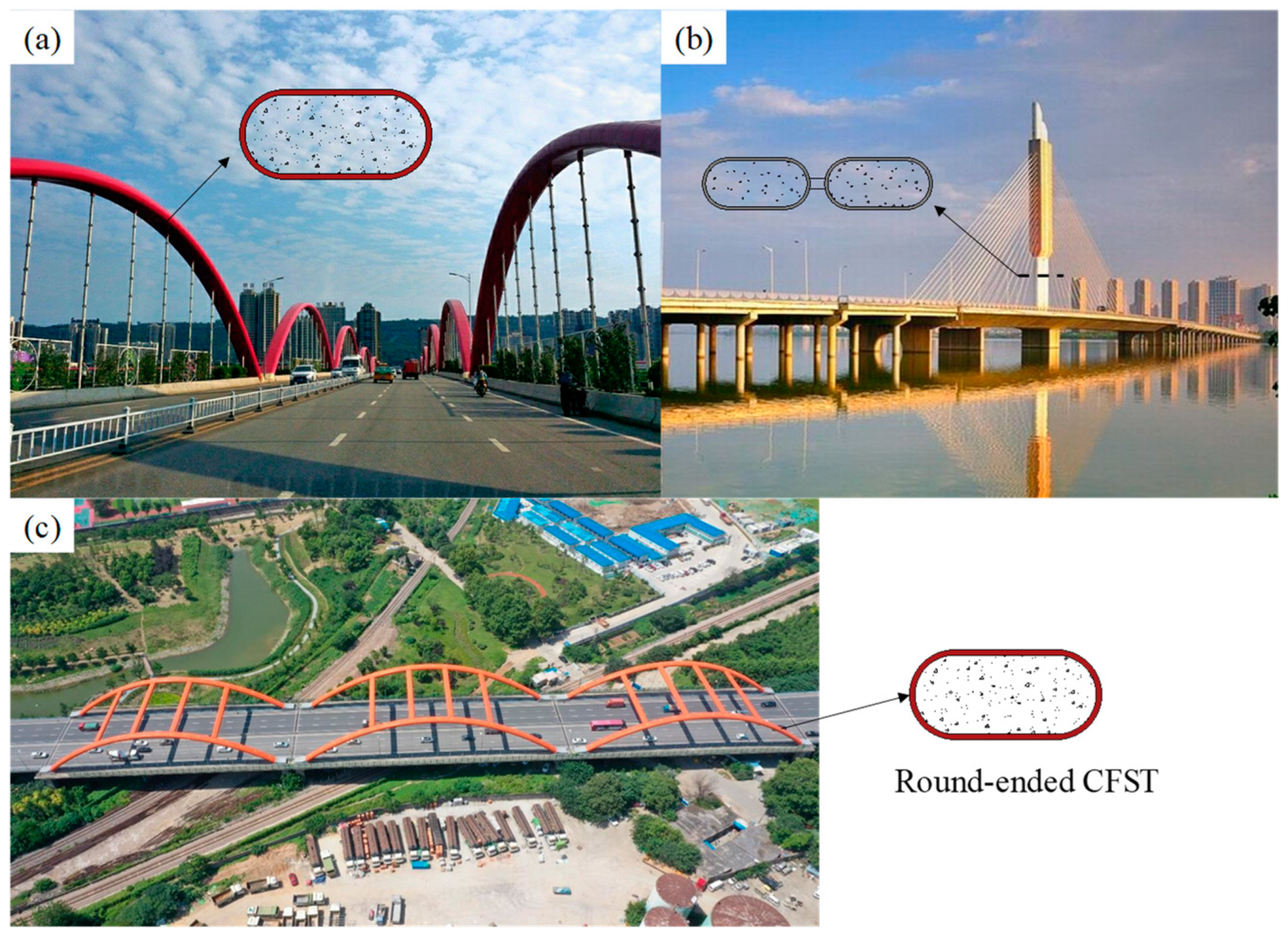
1. Introduction
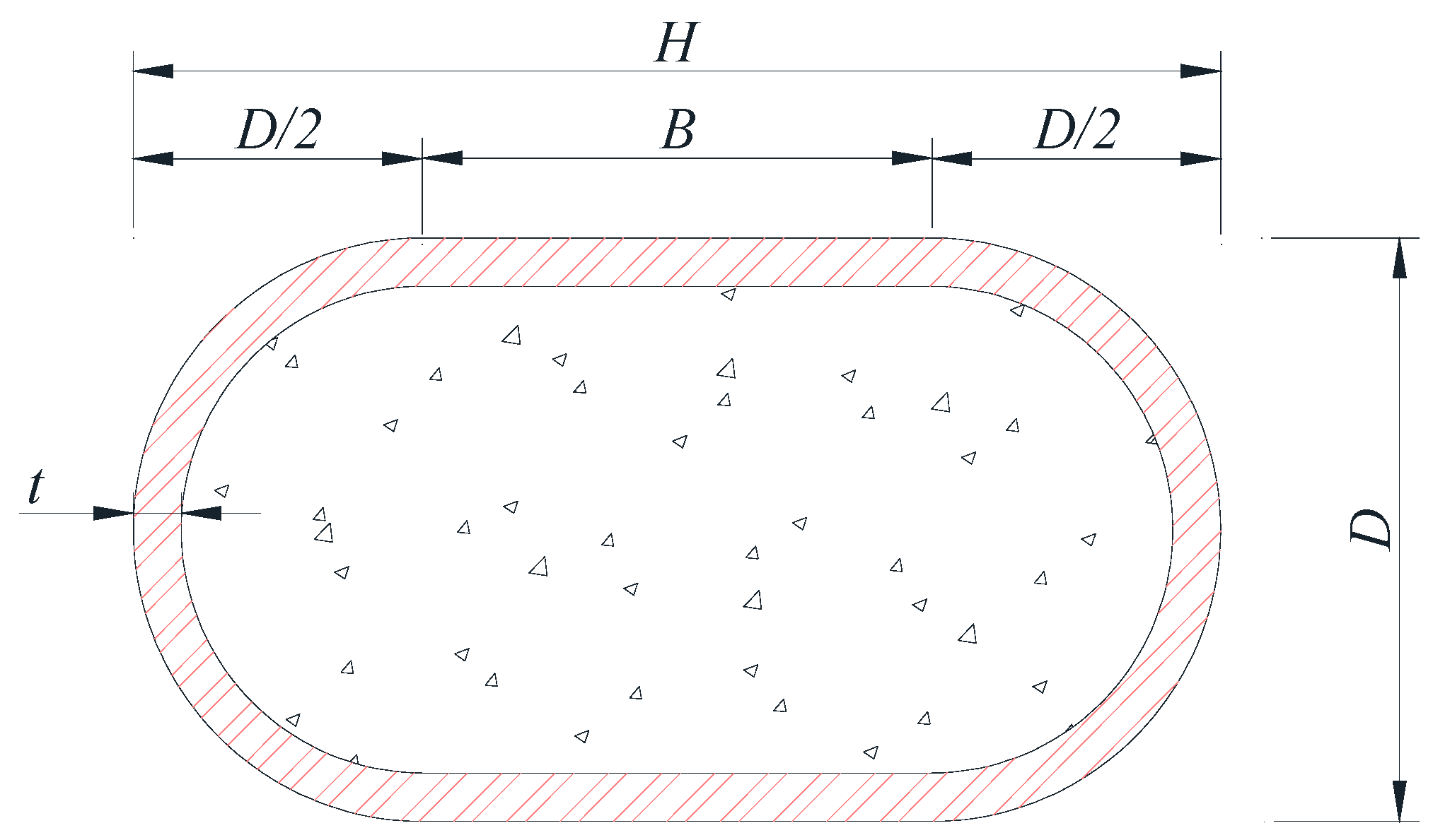
2. Database Establishment
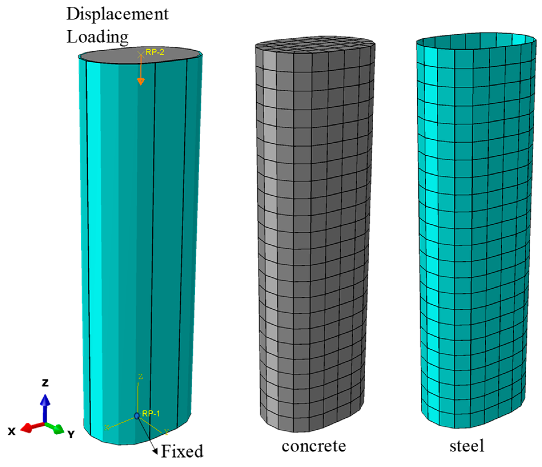
2.1. Finite Element Model
2.1.1. Selection of Elements and Mesh Division
2.1.2. Material and Constitutive Properties
- (1)
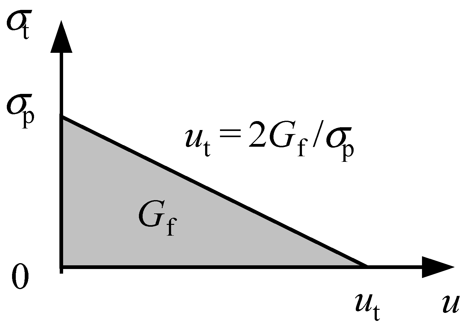
- Concrete
- (2)
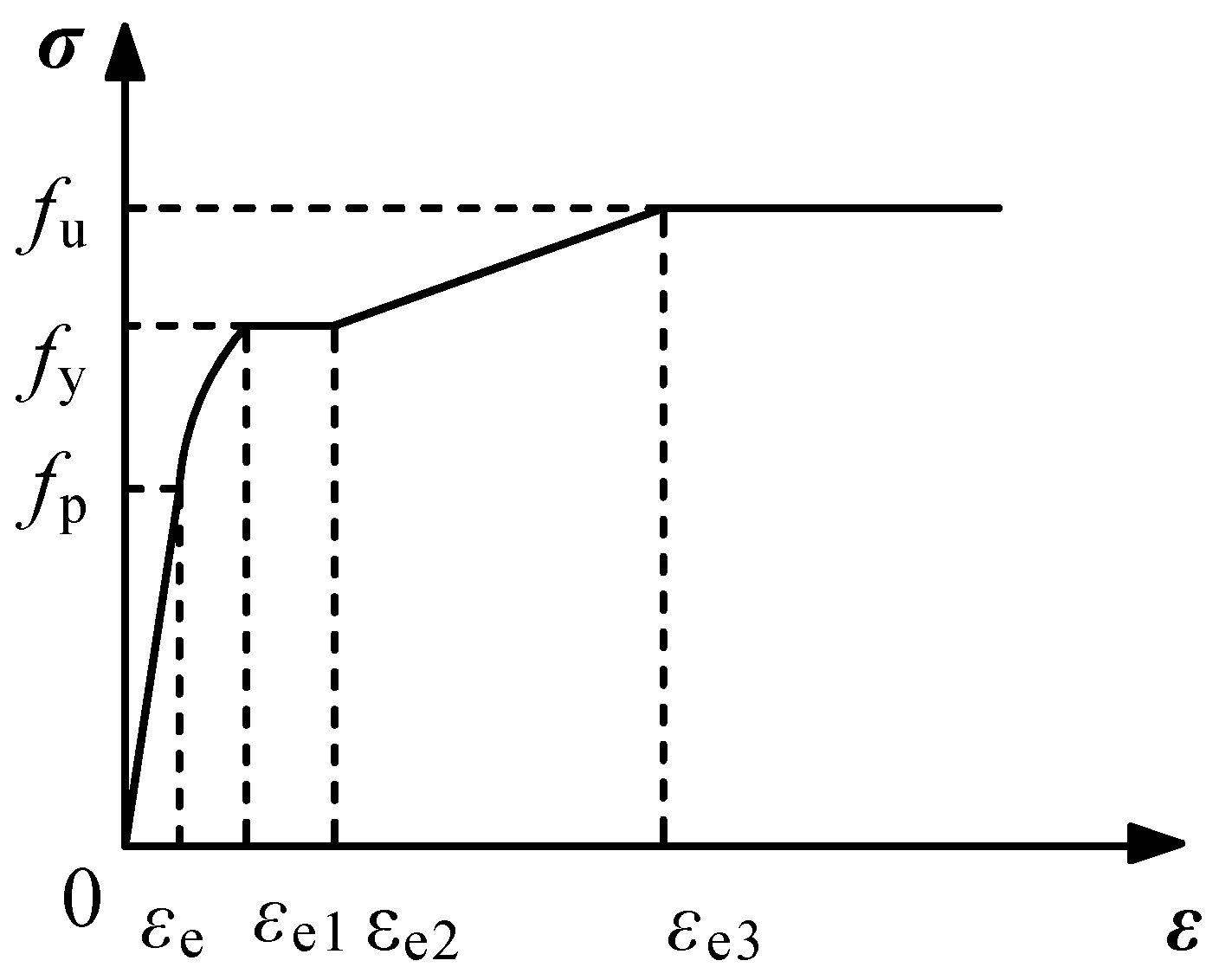
- Steel
2.1.3. Contact and Boundary Conditions
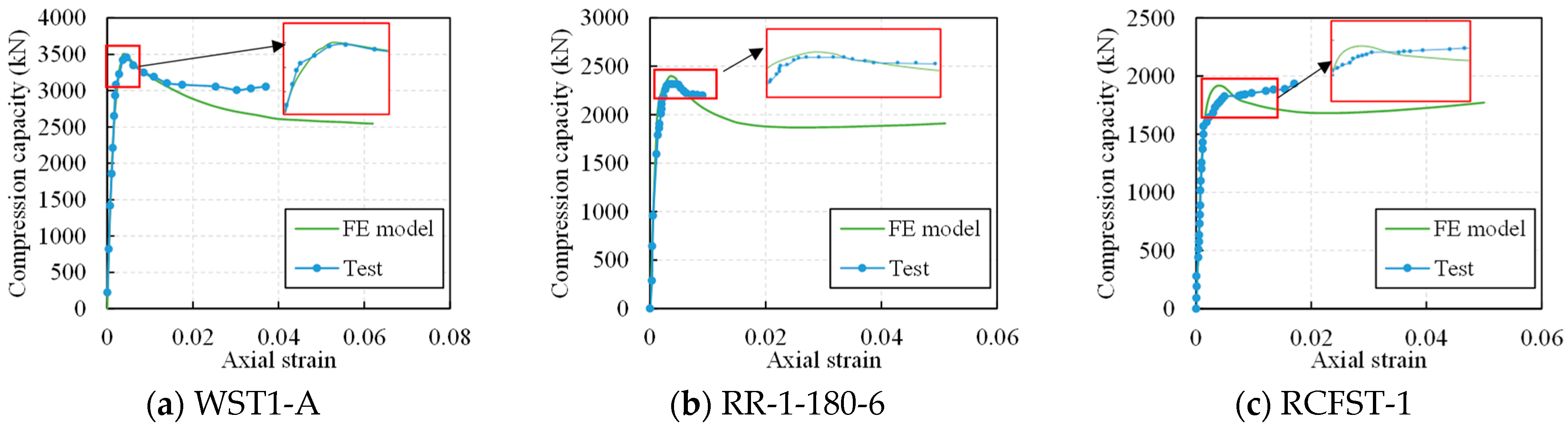
2.2. Verification of FE Model
2.3. Establishment of Machine Learning Database
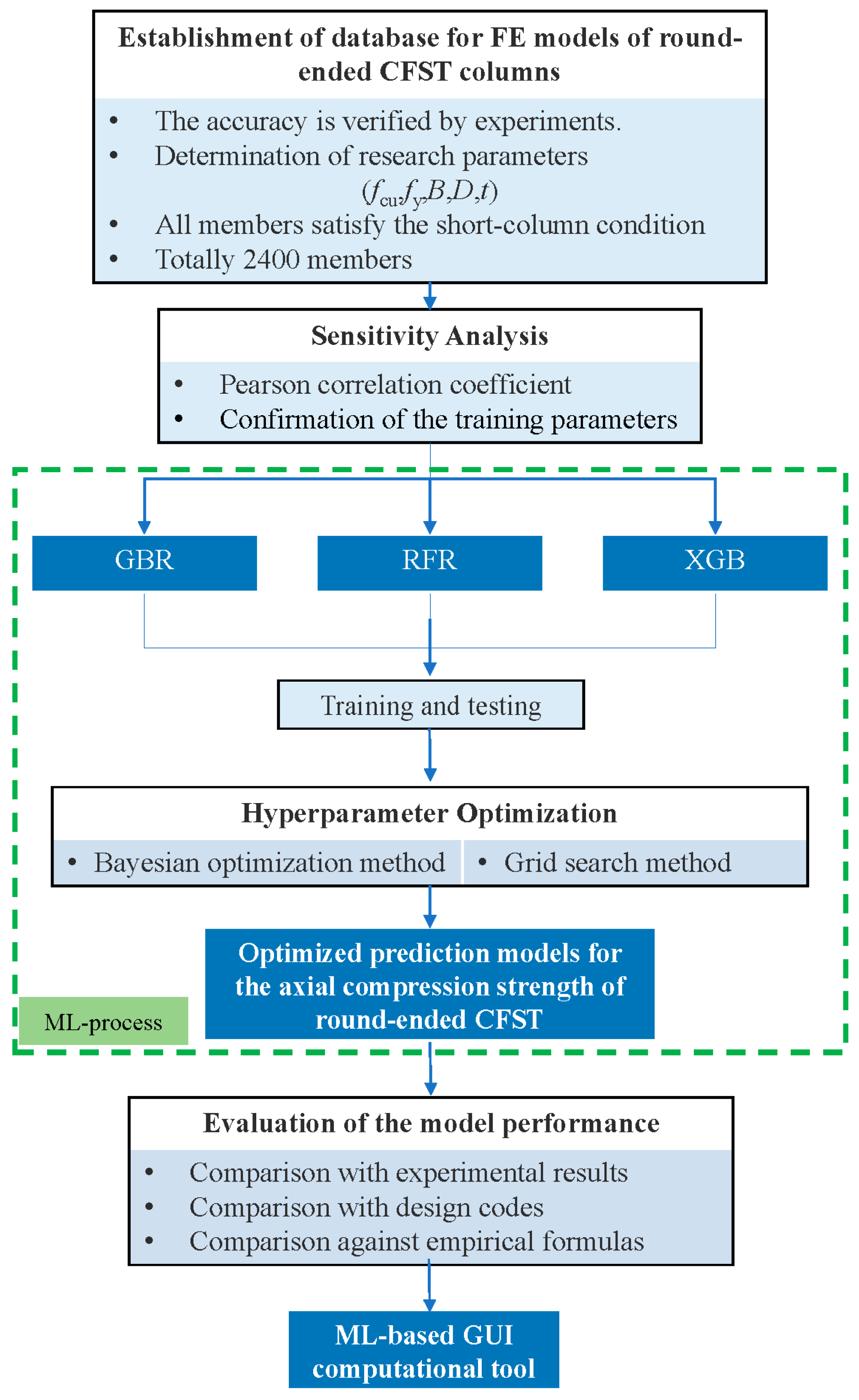
3. Machine Learning
3.1. Sensitivity Analysis
3.2. Selected Algorithm
3.2.1. Gradient Boosting Regression (GBR)
3.2.2. Random Forest Regression (RFR)
3.2.3. Extreme Gradient Boosting (XGB)
3.3. Evaluation Metrics and Hyperparameter Optimization
3.3.1. Evaluation Metrics
- (1)
- Coefficient of determination (R2)
- (2)
- Mean absolute error (MAE)
- (3)
- Root mean square error (RMSE)
- (4)
- Mean (MEAN)
- (5)
- Coefficient of variation (COV)
3.3.2. Hyperparameter Optimization
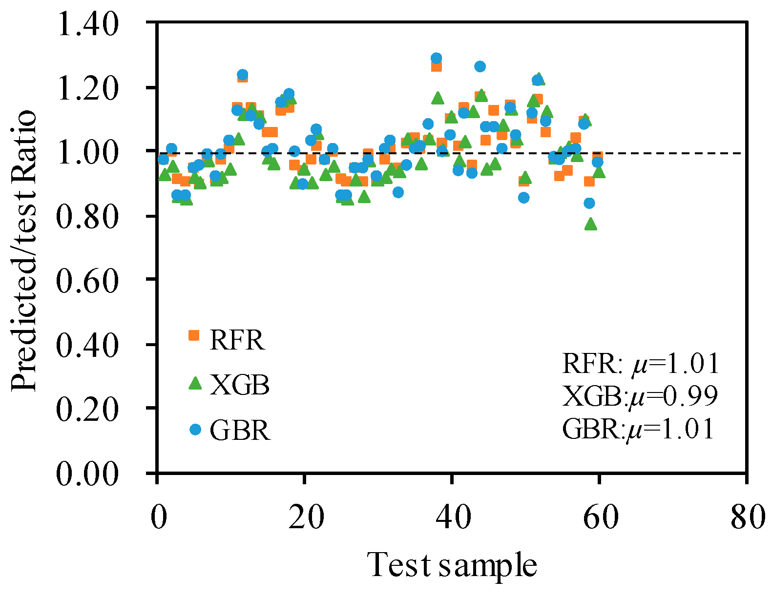
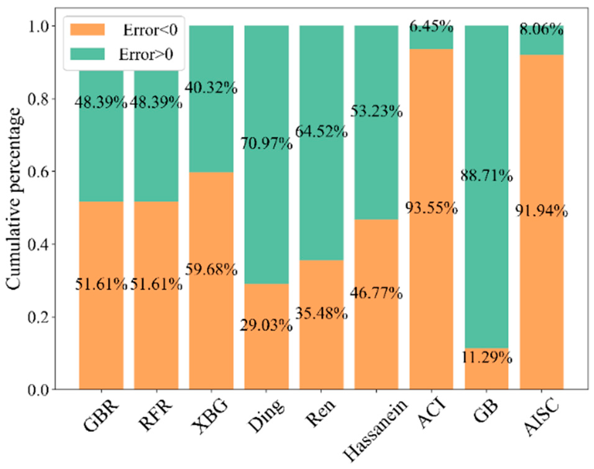
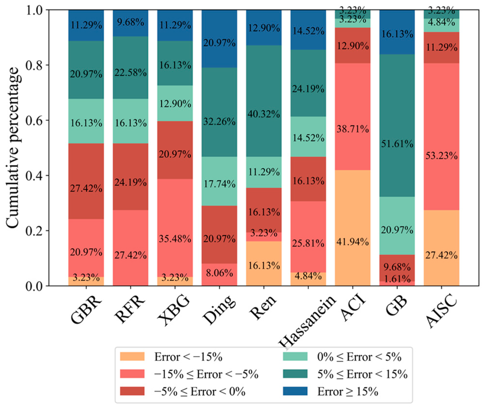
3.4. Comparison of Results
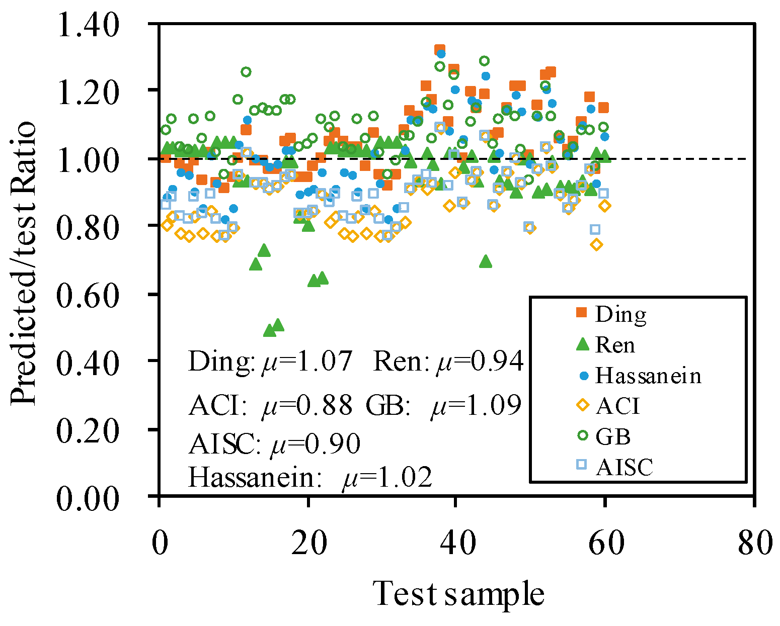
4. Comparison with Existing Calculation Methods
- (1)
- Ding’s formula
- (2)
- Ren’s formula
- (3)
- M.F. Hassanein’s formula
- (4)
- Formula of code ACI 318-11
- (5)
- Formula of code AISC 360-16
- (6)
- Formula of code GB 50936-2014
5. Conclusions
- (1)
- Using the finite element method, a machine learning database comprising 2400 RECFSTs is established. This database encompasses commonly used material strengths and cross-sectional dimensions of RECFST, effectively addressing the issue of insufficient experimental sample size in the current machine learning practices.
- (2)
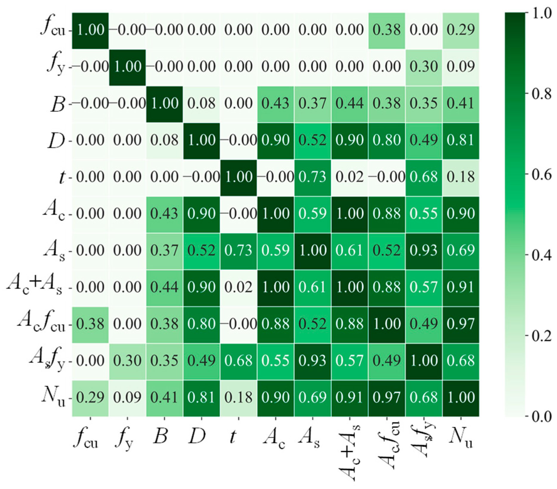
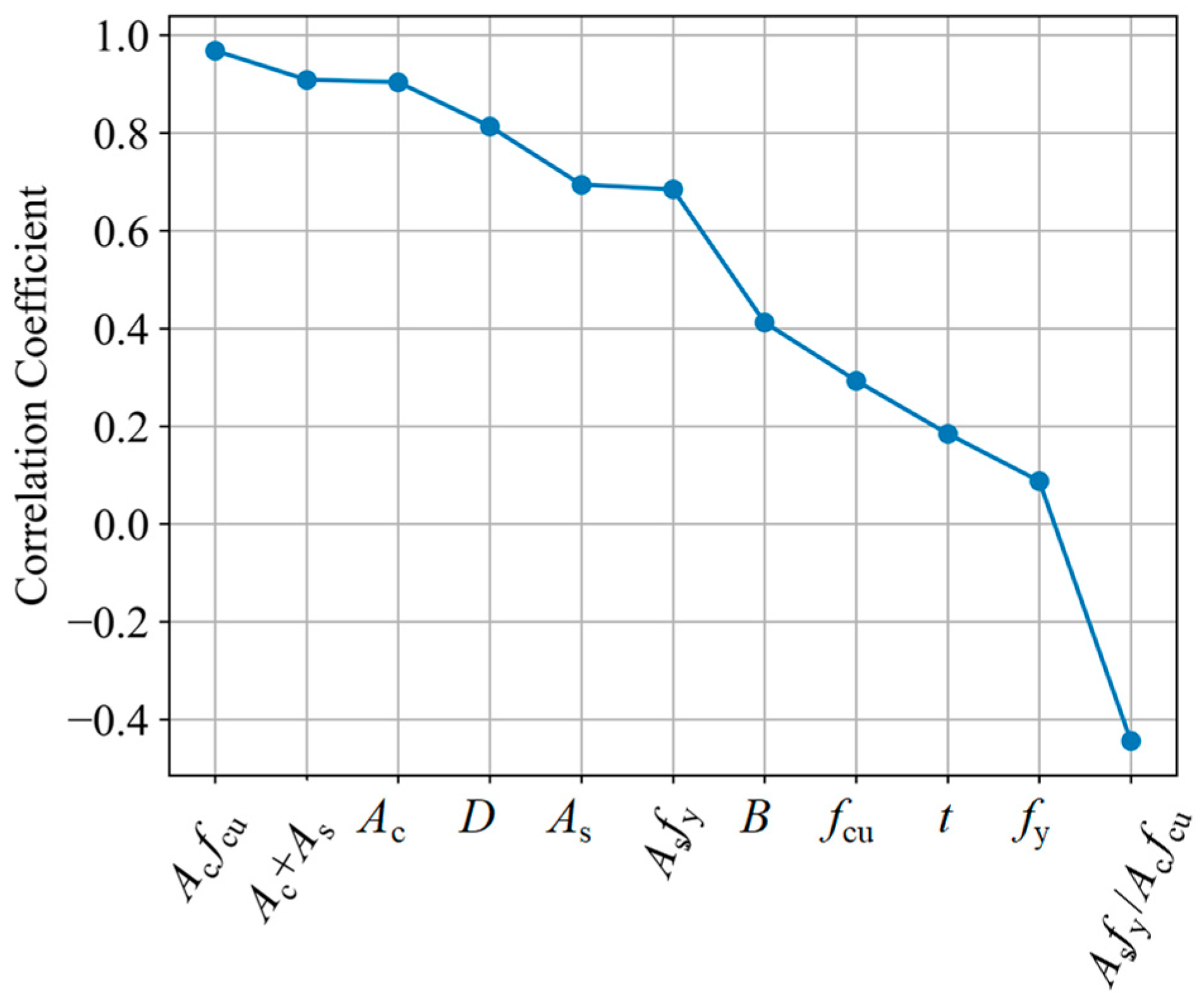
- Through sensitive analysis, in addition to the primary parameter, the second parameters such as Acfcu, Ac + As, Ac, As, and Asfy also show a large correlation with the axial load-bearing capacity Nu, with their Pearson coefficients being 0.968, 0.909, 0.904, 0.694, and 0.684, respectively. Identifying these fundamental parameters closely related to axial load-bearing capacity is an essential foundation for applying machine learning to predict load-bearing capacity.
- (3)
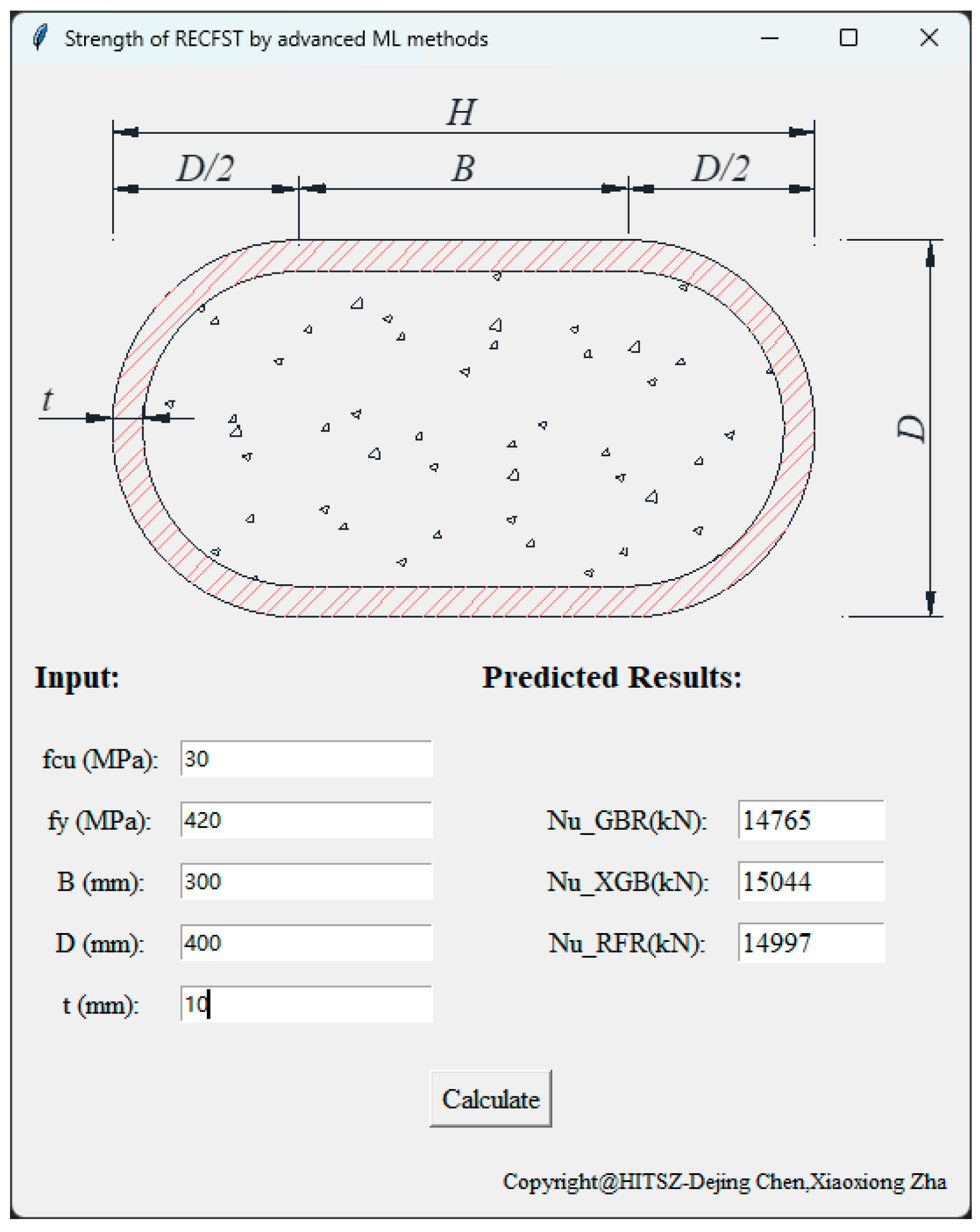
- The three predictive models for the axial load-bearing capacity of RECFST, utilizing advanced machine learning methods, demonstrate higher accuracy compared to the existing theoretical or code-based calculation formulas. Furthermore, they exhibit higher efficiency compared to finite element methods. The development of a graphical user interface (GUI) based on these machine learning prediction models enables the rapid and accurate prediction of the axial load-bearing capacity of RECFST. This development holds significant importance for the engineering applications of RECFST.
Author Contributions
Funding
Data Availability Statement
Conflicts of Interest
Appendix A

| Ref. | Specimens | (kN) | (kN) | (kN) | (kN) | |||
|---|---|---|---|---|---|---|---|---|
| [10] | WST1-A | 3429 | 3436 | 1.00 | 3695 | 1.03 | 3032 | 0.88 |
| WST1-B | 3338 | 3419 | 1.02 | 3685 | 1.03 | 3040 | 0.91 | |
| WST2-A | 4162 | 4101 | 0.99 | 4469 | 1.03 | 3996 | 0.96 | |
| WST2-B | 4168 | 4046 | 0.97 | 4403 | 1.03 | 3955 | 0.95 | |
| WST3-A | 3929 | 3881 | 0.99 | 4157 | 1.02 | 3529 | 0.90 | |
| WST3-B | 4158 | 3879 | 0.93 | 4140 | 1.02 | 3530 | 0.85 | |
| WST4-A | 4492 | 4548 | 1.01 | 4891 | 1.02 | 4543 | 1.01 | |
| WST4-B | 5530 | 5127 | 0.93 | 5542 | 1.05 | 5114 | 0.92 | |
| WST5-A | 5620 | 5107 | 0.91 | 5377 | 1.05 | 4630 | 0.82 | |
| WST5-B | 5500 | 5196 | 0.94 | 5479 | 1.05 | 4699 | 0.85 | |
| WST6-A | 3240 | 3247 | 1.00 | 3376 | 0.93 | 3374 | 1.04 | |
| WST6-B | 2993 | 3237 | 1.08 | 3334 | 0.93 | 3330 | 1.11 | |
| WST7-A | 4826 | 4776 | 0.99 | 3426 | 0.69 | 4809 | 1.00 | |
| WST7-B | 4944 | 4913 | 0.99 | 3721 | 0.73 | 4915 | 0.99 | |
| WST8-A | 6521 | 6282 | 0.96 | 3216 | 0.50 | 6381 | 0.98 | |
| WST8-B | 6493 | 6275 | 0.97 | 3292 | 0.51 | 6367 | 0.98 | |
| WST9-A | 4203 | 4423 | 1.05 | 4468 | 0.99 | 4314 | 1.03 | |
| WST9-B | 4180 | 4405 | 1.05 | 4452 | 0.99 | 4296 | 1.03 | |
| WST10-A | 7201 | 6758 | 0.94 | 5402 | 0.83 | 6442 | 0.89 | |
| WST10-B | 6905 | 6513 | 0.94 | 5076 | 0.81 | 6241 | 0.90 | |
| WST11-A | 9065 | 8853 | 0.98 | 5263 | 0.64 | 8237 | 0.91 | |
| WST11-B | 8799 | 8761 | 1.00 | 5489 | 0.65 | 8420 | 0.96 | |
| [78] | CFRT1-A | 3429 | 3603 | 1.05 | 3709 | 1.03 | 3043 | 0.89 |
| CFRT1-B | 3338 | 3586 | 1.07 | 3690 | 1.03 | 3046 | 0.91 | |
| CFRT2-A | 4162 | 4351 | 1.05 | 4472 | 1.03 | 4000 | 0.96 | |
| CFRT2-B | 4168 | 4293 | 1.03 | 4411 | 1.03 | 3964 | 0.95 | |
| CFRT3-A | 3929 | 4069 | 1.04 | 4158 | 1.02 | 3530 | 0.90 | |
| CFRT3-B | 4158 | 4066 | 0.98 | 4149 | 1.02 | 3537 | 0.85 | |
| CFRT4-A | 4492 | 4825 | 1.07 | 4899 | 1.02 | 4548 | 1.01 | |
| CFRT4-B | 5530 | 5272 | 0.95 | 5543 | 1.05 | 5115 | 0.92 | |
| CFRT5-A | 5620 | 5137 | 0.91 | 5378 | 1.05 | 4631 | 0.82 | |
| CFRT5-B | 5500 | 5225 | 0.95 | 5479 | 1.05 | 4699 | 0.85 | |
| [79] | C1 | 1339 | 1445 | 1.08 | 1476 | 1.02 | 1367 | 1.02 |
| C2 | 1444 | 1647 | 1.14 | 1638 | 0.99 | 1606 | 1.11 | |
| C3 | 1755 | 1968 | 1.12 | 1845 | 0.94 | 1961 | 1.12 | |
| C4 | 1825 | 2218 | 1.22 | 2253 | 1.02 | 2100 | 1.15 | |
| C5 | 2125 | 2495 | 1.17 | 2463 | 0.99 | 2429 | 1.14 | |
| C6 | 2319 | 3056 | 1.32 | 2833 | 0.93 | 3046 | 1.31 | |
| C7 | 1623 | 1789 | 1.10 | 1820 | 1.02 | 1754 | 1.08 | |
| C8 | 1954 | 2471 | 1.26 | 2501 | 1.01 | 2357 | 1.21 | |
| [80] | RCFST-A-0 | 2094 | 2092 | 1.00 | 2037 | 0.97 | 2213 | 1.06 |
| [7] | RCFST-1 | 925 | 1108 | 1.20 | 1116 | 1.01 | 1084 | 1.17 |
| RCFST-2 | 1215 | 1391 | 1.14 | 1296 | 0.93 | 1410 | 1.16 | |
| RCFST-3 | 1635 | 1943 | 1.19 | 1353 | 0.70 | 2034 | 1.24 | |
| RCFST-4 | 1658 | 1768 | 1.07 | 1776 | 1.00 | 1604 | 0.97 | |
| RCFST-5 | 2091 | 2243 | 1.07 | 2104 | 0.94 | 2116 | 1.01 | |
| [21] | RR-1-180-4 | 1755 | 2012 | 1.15 | 1865 | 0.93 | 2010 | 1.15 |
| RR-1-180-6 | 2319 | 2805 | 1.21 | 2538 | 0.90 | 2754 | 1.19 | |
| RR-0.5-180-6 | 1954 | 2361 | 1.21 | 2354 | 1.00 | 2219 | 1.14 | |
| RR-0.5-180-4 | 1623 | 1641 | 1.01 | 1647 | 1.00 | 1589 | 0.98 | |
| [81] | RRCFST-A-180-1 | 2026 | 2345 | 1.16 | 2106 | 0.90 | 2277 | 1.12 |
| RRCFST-A-180-2 | 1915 | 2389 | 1.25 | 2178 | 0.91 | 2308 | 1.21 | |
| RRCFST-C-180-1 | 1574 | 1975 | 1.25 | 1965 | 1.00 | 1830 | 1.16 | |
| [82] | PY1-180-e0-fy235 | 1780 | 1879 | 1.06 | 1730 | 0.92 | 1881 | 1.06 |
| PY1-180-fy345 | 2100 | 2150 | 1.02 | 1969 | 0.92 | 2108 | 1.00 | |
| PYRE1-180-fy345 | 2060 | 2166 | 1.05 | 1974 | 0.91 | 2126 | 1.03 | |
| [83] | RCC1-4-180 | 1755 | 1937 | 1.10 | 1813 | 0.94 | 1925 | 1.10 |
| RCC1-6-180 | 2319 | 2729 | 1.18 | 2493 | 0.91 | 2664 | 1.15 | |
| RCC0.5-4-180 | 1623 | 1569 | 0.97 | 1591 | 1.01 | 1497 | 0.92 | |
| RCC0.5-6-180 | 1954 | 2247 | 1.15 | 2267 | 1.01 | 2075 | 1.06 | |
| Mean | 1.06 | 0.94 | 1.02 | |||||
| Standard deviation | 0.10 | 0.13 | 0.12 |
| Ref. | Specimens | (kN) | (kN) | (kN) | (kN) | |||
|---|---|---|---|---|---|---|---|---|
| [10] | WST1-A | 3429 | 2763 | 0.81 | 3719 | 1.08 | 2960 | 0.86 |
| WST1-B | 3338 | 2771 | 0.83 | 3730 | 1.12 | 2968 | 0.89 | |
| WST2-A | 4162 | 3245 | 0.78 | 4305 | 1.03 | 3444 | 0.83 | |
| WST2-B | 4168 | 3216 | 0.77 | 4266 | 1.02 | 3413 | 0.82 | |
| WST3-A | 3929 | 3251 | 0.83 | 4387 | 1.12 | 3491 | 0.89 | |
| WST3-B | 4158 | 3249 | 0.78 | 4383 | 1.05 | 3488 | 0.84 | |
| WST4-A | 4492 | 3780 | 0.84 | 5029 | 1.12 | 4019 | 0.89 | |
| WST4-B | 5530 | 4253 | 0.77 | 5605 | 1.01 | 4548 | 0.82 | |
| WST5-A | 5620 | 4323 | 0.77 | 5347 | 0.95 | 4323 | 0.77 | |
| WST5-B | 5500 | 4393 | 0.80 | 5436 | 0.99 | 4393 | 0.80 | |
| WST6-A | 3240 | 3093 | 0.95 | 3805 | 1.17 | 3093 | 0.95 | |
| WST6-B | 2993 | 3051 | 1.02 | 3754 | 1.25 | 3051 | 1.02 | |
| WST7-A | 4826 | 4454 | 0.92 | 5509 | 1.14 | 4454 | 0.92 | |
| WST7-B | 4944 | 4563 | 0.92 | 5654 | 1.14 | 4563 | 0.92 | |
| WST8-A | 6521 | 5957 | 0.91 | 7408 | 1.14 | 5957 | 0.91 | |
| WST8-B | 6493 | 5945 | 0.92 | 7405 | 1.14 | 5945 | 0.92 | |
| WST9-A | 4203 | 3975 | 0.95 | 4921 | 1.17 | 3975 | 0.95 | |
| WST9-B | 4180 | 3959 | 0.95 | 4905 | 1.17 | 3959 | 0.95 | |
| WST10-A | 7201 | 5997 | 0.83 | 7460 | 1.04 | 5997 | 0.83 | |
| WST10-B | 6905 | 5793 | 0.84 | 7199 | 1.04 | 5793 | 0.84 | |
| WST11-A | 9065 | 7688 | 0.85 | 9593 | 1.06 | 7688 | 0.85 | |
| WST11-B | 8799 | 7873 | 0.89 | 9816 | 1.12 | 7873 | 0.89 | |
| [78] | CFRT1-A | 3429 | 2774 | 0.81 | 3735 | 1.09 | 2972 | 0.87 |
| CFRT1-B | 3338 | 2776 | 0.83 | 3737 | 1.12 | 2974 | 0.89 | |
| CFRT2-A | 4162 | 3248 | 0.78 | 4309 | 1.04 | 3447 | 0.83 | |
| CFRT2-B | 4168 | 3224 | 0.77 | 4278 | 1.03 | 3422 | 0.82 | |
| CFRT3-A | 3929 | 3252 | 0.83 | 4388 | 1.12 | 3492 | 0.89 | |
| CFRT3-B | 4158 | 3256 | 0.78 | 4393 | 1.06 | 3496 | 0.84 | |
| CFRT4-A | 4492 | 3785 | 0.84 | 5035 | 1.12 | 4024 | 0.90 | |
| CFRT4-B | 5530 | 4254 | 0.77 | 5606 | 1.01 | 4549 | 0.82 | |
| CFRT5-A | 5620 | 4324 | 0.77 | 5348 | 0.95 | 4324 | 0.77 | |
| CFRT5-B | 5500 | 4393 | 0.80 | 5436 | 0.99 | 4393 | 0.80 | |
| [79] | C1 | 1339 | 1086 | 0.81 | 1422 | 1.06 | 1146 | 0.86 |
| C2 | 1444 | 1310 | 0.91 | 1538 | 1.06 | 1310 | 0.91 | |
| C3 | 1755 | 1641 | 0.94 | 1944 | 1.11 | 1641 | 0.94 | |
| C4 | 1825 | 1654 | 0.91 | 2127 | 1.17 | 1733 | 0.95 | |
| C5 | 2125 | 1960 | 0.92 | 2245 | 1.06 | 1960 | 0.92 | |
| C6 | 2319 | 2526 | 1.09 | 2936 | 1.27 | 2526 | 1.09 | |
| C7 | 1623 | 1402 | 0.86 | 1868 | 1.15 | 1493 | 0.92 | |
| C8 | 1954 | 1873 | 0.96 | 2425 | 1.24 | 1966 | 1.01 | |
| [80] | RCFST-A-0 | 2094 | 1816 | 0.87 | 2171 | 1.04 | 1816 | 0.87 |
| [7] | RCFST-1 | 925 | 866 | 0.94 | 1022 | 1.10 | 866 | 0.94 |
| RCFST-2 | 1215 | 1164 | 0.96 | 1392 | 1.15 | 1164 | 0.96 | |
| RCFST-3 | 1635 | 1739 | 1.06 | 2100 | 1.28 | 1739 | 1.06 | |
| RCFST-4 | 1658 | 1422 | 0.86 | 1729 | 1.04 | 1422 | 0.86 | |
| RCFST-5 | 2091 | 1903 | 0.91 | 2335 | 1.12 | 1903 | 0.91 | |
| [21] | RR-1-180-4 | 1755 | 1688 | 0.96 | 2001 | 1.14 | 1688 | 0.96 |
| RR-1-180-6 | 2319 | 2315 | 1.00 | 2609 | 1.13 | 2315 | 1.00 | |
| RR-0.5-180-6 | 1954 | 1804 | 0.92 | 2008 | 1.03 | 1804 | 0.92 | |
| RR-0.5-180-4 | 1623 | 1292 | 0.80 | 1516 | 0.93 | 1292 | 0.80 | |
| [81] | RRCFST-A-180-1 | 2026 | 1956 | 0.97 | 2281 | 1.13 | 1956 | 0.97 |
| RRCFST-A-180-2 | 1915 | 1983 | 1.04 | 2316 | 1.21 | 1983 | 1.04 | |
| RRCFST-C-180-1 | 1574 | 1532 | 0.97 | 1767 | 1.12 | 1532 | 0.97 | |
| [82] | PY1-180-e0-fy235 | 1780 | 1586 | 0.89 | 1896 | 1.07 | 1586 | 0.89 |
| PY1-180-fy345 | 2100 | 1796 | 0.86 | 2110 | 1.00 | 1796 | 0.86 | |
| PYRE1-180-fy345 | 2060 | 1813 | 0.88 | 2131 | 1.03 | 1813 | 0.88 | |
| [83] | RCC1-4-180 | 1755 | 1614 | 0.92 | 1904 | 1.08 | 1614 | 0.92 |
| RCC1-6-180 | 2319 | 2237 | 0.96 | 2510 | 1.08 | 2237 | 0.96 | |
| RCC0.5-4-180 | 1623 | 1208 | 0.74 | 1584 | 0.98 | 1276 | 0.79 | |
| RCC0.5-6-180 | 1954 | 1674 | 0.86 | 2134 | 1.09 | 1744 | 0.89 | |
| Mean | 0.88 | 1.09 | 0.90 | |||||
| Standard deviation | 0.08 | 0.08 | 0.07 |
References
- Long, Y.-L.; Zeng, L. A refined model for local buckling of rectangular CFST columns with binding bars. Thin Walled Struct. 2018, 132, 431–441. [Google Scholar] [CrossRef]
- Long, Y.-L.; Wan, J.; Cai, J. Theoretical study on local buckling of rectangular CFT columns under eccentric compression. J. Constr. Steel Res. 2016, 120, 70–80. [Google Scholar] [CrossRef]
- Wang, Q.-K.; Chen, M.; Lu, Z.-A. Finite element analysis for the mechanical behaviors of circle-ended concrete-filled steel tubular tower. In Proceedings of the 2009 Second International Conference on Information and Computing Science, Manchester, UK, 21–22 May 2009; pp. 110–113. [Google Scholar]
- Xie, J.X.; Lu, Z.A.; Tang, P.; Liu, D. Modal Analysis and Experimental Study on Round-Ended CFST Coupled Column Cable Stayed Bridge. In Proceedings of the 2011 Second International Conference on Mechanic Automation and Control Engineering, Inner Mongolia, China, 15–17 July 2011; pp. 2302–2304. [Google Scholar]
- Xie, J.-X.; Lu, Z.-A. Numerical Simulation and Test Study on Non-Uniform Area of Round-Ended CFST Tubular Tower. In Proceedings of the 2010 Third International Conference on Information and Computing, Wuxi, China, 4–6 June 2010; pp. 19–22. [Google Scholar]
- Xie, J.X.; Lu, Z.A. Test Study and Contact Analysis of Round-Ended CFST Coupled Column. In Proceedings of the 2nd International Conference on Model and Simulation, Rome, Italy, 2–6 March 2009. pp. 28–32.
- Wang, Z.B.; Chen, J.; Xie, E.P.; Lin, S. Behavior of concrete-filled round-end steel tubular stubcolumns under axial compression. J. Build. Structures 2014, 35, 123–130. (In Chinese) [Google Scholar]
- Guo, J.-T.; Wang, Z.-B.; Tan, E.L.; Gao, Y.-H. Flexural performance of round-ended concrete-filled steel tubular specimens. J. Constr. Steel Res. 2024, 215, 108529. [Google Scholar] [CrossRef]
- Ding, F.X.; Zhang, T.; Wang, L.; Fu, L. Further analysis on the flexural behavior of concrete-filled round-ended steel tubes. Steel Compos. Struct. 2019, 30, 149–169. [Google Scholar]
- Faxing, D.; Lei, F.; Zhiwu, Y.; Gang, L. Mechanical performances of concrete-filled steel tubular stub columns with round ends under axial loading. Thin-Walled Struct. 2015, 97, 22–34. [Google Scholar] [CrossRef]
- Ding, F.; Xiong, S.; Zhang, H.; Li, G.; Zhao, P.; Xiang, P. Reliability analysis of axial bearing capacity of concrete filled steel tubular stub columns with different cross sections. Structures 2021, 33, 4193–4202. [Google Scholar] [CrossRef]
- Shen, Q.; Wang, F.; Wang, J.; Ma, X. Cyclic behaviour and design of cold-formed round-ended concrete-filled steel tube columns. J. Constr. Steel Res. 2022, 190, 107089. [Google Scholar] [CrossRef]
- Shen, Q.; Wang, J.; Liew, J.R.; Gao, B.; Xiao, Q. Experimental study and strength evaluation of axially loaded welded tubular joints with round-ended oval hollow sections. Thin-Walled Struct. 2020, 154, 106846. [Google Scholar] [CrossRef]
- Wang, J.; Shen, Q. Numerical analysis and design of thin-walled RECFST stub columns under axial compression. Thin-Walled Struct. 2018, 129, 166–182. [Google Scholar] [CrossRef]
- Shen, Q.H.; Wang, J.F.; Wang, W.Q.; Wang, Z.B. Performance and design of eccentrically-loaded concrete-filled round-ended elliptical hollow section stub columns. J. Constr. Steel Res. 2018, 150, 99–114. [Google Scholar] [CrossRef]
- Xing, W.B.; Shen, Q.H.; Wang, J.F.; Sheng, M.Y. Performance and design of oval-ended elliptical CFT columns under combined axial compression-torsion. J. Constr. Steel Res. 2020, 172, 106148. [Google Scholar] [CrossRef]
- Wang, R.; Li, X.; Zhao, H.; Wang, Y.H.; Lam, D.; Chen, M.T. Eccentric compression performance of round-ended CFST slender columns with different aspect ratios. J. Constr. Steel Res. 2023, 211, 108198. [Google Scholar] [CrossRef]
- Zhao, H.; Mei, S.Q.; Wang, R.; Yang, X.; Lam, D.; Chen, W.S. Round-ended concrete-filled steel tube columns under impact loading: Test, numerical analysis and design method. Thin-Walled Struct. 2023, 191, 111020. [Google Scholar] [CrossRef]
- Zhao, H.; Mei, S.Q.; Wang, R.; Yang, X.; Wang, W.D.; Chen, W.S. Performance of round-ended CFST columns under combined actions of eccentric compression and impact loads. Eng. Struct. 2024, 301, 117328. [Google Scholar] [CrossRef]
- Zhao, H.; Zhang, W.H.; Wang, R.; Hou, C.C.; Lam, D. Axial compression behaviour of round-ended recycled aggregate concrete-filled steel tube stub columns (RE-RACFST): Experiment, numerical modeling and design. Eng. Struct. 2023, 276, 115376. [Google Scholar] [CrossRef]
- Ren, Z.G.; Wang, D.D.; Li, P.P. Axial compressive behaviour and confinement effect of round-ended rectangular CFST with different central angles. Compos. Struct. 2022, 285, 115193. [Google Scholar] [CrossRef]
- Hassanein, M.F.; Patel, V.I. Round-ended rectangular concrete-filled steel tubular short columns: FE investigation under axial compression. J. Constr. Steel Res. 2018, 140, 222–236. [Google Scholar] [CrossRef]
- Piquer, A.; Ibañez, C.; Hernández-Figueirido, D. Structural response of concrete-filled round-ended stub columns subjected to eccentric loads. Eng. Struct. 2019, 184, 318–328. [Google Scholar] [CrossRef]
- Patel, V.I. Analysis of uniaxially loaded short round-ended concrete-filled steel tubular beam-columns. Eng. Struct. 2020, 205, 110098. [Google Scholar] [CrossRef]
- Zhang, Q.; Fu, L.; Xu, L. An efficient approach for numerical simulation of concrete-filled round-ended steel tubes. J. Constr. Steel Res. 2020, 170, 106086. [Google Scholar] [CrossRef]
- Ahmed, M.; Liang, Q.Q. Numerical analysis of thin-walled round-ended concrete-filled steel tubular short columns including local buckling effects. Structures 2020, 28, 181–196. [Google Scholar] [CrossRef]
- Ahmed, M.; Liang, Q.Q.; Patel, V.I.; Gohari, S.; Hamoda, A. Unified numerical model for performance analysis of various cross-sections of concrete-filled stainless-steel tubular stub columns under axial loading. Structures 2023, 55, 799–817. [Google Scholar] [CrossRef]
- Jordan, M.I.; Mitchell, T.M. Machine learning: Trends, perspectives, and prospects. Science 2015, 349, 255–260. [Google Scholar] [CrossRef] [PubMed]
- Yu, Y.; Liang, S.; Samali, B.; Nguyen, T.N.; Zhai, C.; Li, J.; Xie, X. Torsional capacity evaluation of RC beams using an improved bird swarm algorithm optimised 2D convolutional neural network. Eng. Struct. 2022, 273, 115066. [Google Scholar] [CrossRef]
- Yu, Y.; Zhang, C.; Xie, X.; Yousefi, A.M.; Zhang, G.; Li, J.; Samali, B. Compressive strength evaluation of cement-based materials in sulphate environment using optimized deep learning technology. Dev. Built. Environ. 2023, 16, 100298. [Google Scholar] [CrossRef]
- Güneyisi, E.M.; Gültekin, A.; Mermerdaş, K. Ultimate capacity prediction of axially loaded CFST short columns. Int. J. Steel Struct. 2016, 16, 99–114. [Google Scholar] [CrossRef]
- Hou, C.; Zhou, X.G. Strength prediction of circular CFST columns through advanced machine learning methods. J. Build. Eng. 2022, 51, 104289. [Google Scholar] [CrossRef]
- Ngo, N.-T.; Le, H.A.; Pham, T.-P. Integration of support vector regression and grey wolf optimization for estimating the ultimate bearing capacity in concrete-filled steel tube columns. Neural Comput. Appl. 2021, 33, 8525–8542. [Google Scholar] [CrossRef]
- Nguyen, M.-S.T.; Trinh, M.-C.; Kim, S.-E. Uncertainty quantification of ultimate compressive strength of CCFST columns using hybrid machine learning model. Eng. Comput. 2022, 38, 2719–2738. [Google Scholar] [CrossRef]
- Sarir, P.; Chen, J.; Asteris, P.G.; Armaghani, D.J.; Tahir, M.M. Developing GEP tree-based, neuro-swarm, and whale optimization models for evaluation of bearing capacity of concrete-filled steel tube columns. Eng. Comput. 2021, 37, 1–19. [Google Scholar] [CrossRef]
- Sarir, P.; Shen, S.-L.; Wang, Z.-F.; Chen, J.; Horpibulsuk, S.; Pham, B.T. Optimum model for bearing capacity of concrete-steel columns with AI technology via incorporating the algorithms of IWO and ABC. Eng. Comput. 2021, 37, 797–807. [Google Scholar] [CrossRef]
- Degtyarev, V.V.; Thai, H.T. Design of concrete-filled steel tubular columns using data-driven methods. J. Constr. Steel Res. 2023, 200, 107653. [Google Scholar] [CrossRef]
- Duong, T.H.; Le, T.-T.; Le, M.V. Practical Machine Learning Application for Predicting Axial Capacity of Composite Concrete-Filled Steel Tube Columns Considering Effect of Cross-Sectional Shapes. Int. J. Steel Struct. 2023, 23, 263–278. [Google Scholar] [CrossRef]
- Le, T.-T.; Phan, H.C. Prediction of Ultimate Load of Rectangular CFST Columns Using Interpretable Machine Learning Method. Adv. Civ. Eng. 2020, 2020, e8855069. [Google Scholar] [CrossRef]
- Nguyen, T.-A.; Trinh, S.H.; Nguyen, M.H.; Ly, H.-B. Novel ensemble approach to predict the ultimate axial load of CFST columns with different cross-sections. Structures 2023, 47, 1–14. [Google Scholar] [CrossRef]
- Nguyen, T.; Le Nguyen, K.; Ly, H. Universal boosting ML approaches to predict the ultimate load capacity of CFST columns. Struct. Des. Tall Spec. Build. 2024, 33, e2071. [Google Scholar] [CrossRef]
- Tran, V.L.; Jang, Y.; Kim, S.E. Improving the axial compression capacity prediction of elliptical CFST columns using a hybrid ANN-IP model. Steel Compos. Struct. 2021, 39, 319–335. [Google Scholar]
- Zarringol, M.; Thai, H.T. Prediction of the load-shortening curve of CFST columns using ANN-based models. J. Build. Eng. 2022, 51, 104279. [Google Scholar] [CrossRef]
- Zhou, X.-G.; Hou, C.; Feng, W.-Q. Optimized data-driven machine learning models for axial strength prediction of rectangular CFST columns. Structures 2023, 47, 760–780. [Google Scholar] [CrossRef]
- Zhou, X.-G.; Hou, C.; Peng, J. Active learning methods for strength assessment of circular CFST under coupled long-term axial loading and random localized corrosion. Thin-Walled Struct. 2023, 193, 111254. [Google Scholar] [CrossRef]
- Hanoon, A.N.; Al Zand, A.W.; Yaseen, Z.M. Designing new hybrid artificial intelligence model for CFST beam flexural performance prediction. Eng. Comput. 2022, 38, 3109–3135. [Google Scholar] [CrossRef]
- Hou, C.; Zhou, X.-G.; Shen, L. Intelligent prediction methods for N–M interaction of CFST under eccentric compression. Arch. Civ. Mech. Eng. 2023, 23, 197. [Google Scholar] [CrossRef]
- Huang, H.; Xue, C.; Zhang, W.; Guo, M. Torsion design of CFRP-CFST columns using a data-driven optimization approach. Eng. Struct. 2022, 251, 113479. [Google Scholar] [CrossRef]
- Wang, C.; Chan, T.M. Machine learning (ML) based models for predicting the ultimate strength of rectangular concrete-filled steel tube (CFST) columns under eccentric loading. Eng. Struct. 2023, 276, 115392. [Google Scholar] [CrossRef]
- Zarringol, M.; Thai, H.-T.; Naser, M. Application of machine learning models for designing CFCFST columns. J. Constr. Steel Res. 2021, 185, 106856. [Google Scholar] [CrossRef]
- Zarringol, M.; Patel, V.I.; Liang, Q.Q.; Hassanein, M.F.; Ahmed, M. Machine-learning-based predictive models for concrete-filled double skin tubular columns. Eng. Struct. 2024, 304, 117593. [Google Scholar] [CrossRef]
- Hong, Z.-T.; Wang, W.-D.; Zheng, L.; Shi, Y.-L. Machine learning models for predicting axial compressive capacity of circular CFDST columns. Structures 2023, 57, 105285. [Google Scholar] [CrossRef]
- Miao, K.; Pan, Z.; Chen, A.; Wei, Y.; Zhang, Y. Machine learning-based model for the ultimate strength of circular concrete-filled fiber-reinforced polymer–steel composite tube columns. Constr. Build. Mater. 2023, 394, 132134. [Google Scholar] [CrossRef]
- Zarringol, M.; Patel, V.I.; Liang, Q.Q. Artificial neural network model for strength predictions of CFST columns strengthened with CFRP. Eng. Struct. 2023, 281, 115784. [Google Scholar] [CrossRef]
- Chen, K.; Wang, S.; Wang, Y.; Wei, J.; Wang, Q.; Du, W.; Jin, W. Intelligent design of limit states for recycled aggregate concrete filled steel tubular columns. Structures 2023, 58, 105338. [Google Scholar] [CrossRef]
- Zhou, X.-G.; Hou, C.; Peng, J.; Yao, G.-H.; Fang, Z. Structural mechanism-based intelligent capacity prediction methods for concrete-encased CFST columns. J. Constr. Steel Res. 2023, 202, 107769. [Google Scholar] [CrossRef]
- Han, L.-H.; Yao, G.-H.; Tao, Z. Performance of concrete-filled thin-walled steel tubes under pure torsion. Thin-Walled Struct. 2007, 45, 24–36. [Google Scholar] [CrossRef]
- Hillerborg, A.; Modéer, M.; Petersson, P.-E. Analysis of crack formation and crack growth in concrete by means of fracture mechanics and finite elements. Cem. Concr. Res. 1976, 6, 773–781. [Google Scholar] [CrossRef]
- Jiang, J.J.; Lu, X.Z.; Ye, L.P. Finite Element Analysis of Concrete Structures; Beijing Tsinhhua University Press: Beijing, China, 2005. (In Chinese) [Google Scholar]
- Shen, J.M.; Wang, C.Z.; Jiang, J.Q. Finite Element Analysis of Reinforced Concrete and Limit Analysis of Plates and Shells; Tsinhhua University Press: Beijing, China, 1993. (In Chinese) [Google Scholar]
- Hu, H.-T.; Huang, C.-S.; Wu, M.-H.; Wu, Y.-M. Nonlinear analysis of axially loaded concrete-filled tube columns with confinement effect. J. Struct. Eng. 2003, 129, 1322–1329. [Google Scholar] [CrossRef]
- Lin, S.; Zhao, Y.-G. Numerical study of the behaviors of axially loaded large-diameter CFT stub columns. J. Constr. Steel Res. 2019, 160, 54–66. [Google Scholar] [CrossRef]
- Guo, L.; Zhang, S.; Kim, W.-J.; Ranzi, G. Behavior of square hollow steel tubes and steel tubes filled with concrete. Thin-Walled Struct. 2007, 45, 961–973. [Google Scholar] [CrossRef]
- Nassiraei, H. Probabilistic Analysis of Strength in Retrofitted X-Joints under Tensile Loading and Fire Conditions. Buildings 2024, 14, 2105. [Google Scholar] [CrossRef]
- Yu, M. Research on the Consecutive Theory of Concrete-Filled Steel Members Under Normal to High Temperature and Impact Load. Ph.D. Thesis, Harbin Institute of Technology, Harbin, China, 2011. (In Chinese). [Google Scholar]
- Han, L.-H.; Li, W.; Bjorhovde, R. Developments and advanced applications of concrete-filled steel tubular (CFST) structures: Members. J. Constr. Steel Res. 2014, 100, 211–228. [Google Scholar] [CrossRef]
- Evirgen, B.; Tuncan, A.; Taskin, K. Structural behavior of concrete filled steel tubular sections (CFT/CFSt) under axial compression. Thin-Walled Struct. 2014, 80, 46–56. [Google Scholar] [CrossRef]
- GB50017-2017; Standard for Design of Steel Structures. China Architecture & Building Press: Beijing, China, 2017. (In Chinese)
- GB 50010-2010; Code for Design of Concrete Structures. China Architecture & Building Press: Beijing, China, 2015. (In Chinese)
- Chen, D.; Zha, X.; Fan, Y. Theoretical and experimental investigations on the stability performance of concrete-filled steel tubular X-column with regard to the flexural rigidity variation. J. Build. Eng. 2023, 78, 107698. [Google Scholar] [CrossRef]
- Pearson, K., VII. Note on regression and inheritance in the case of two parents. Proc. R. Soc. Lond. 1895, 58, 240–242. [Google Scholar]
- ACI 318-11; Building Code Requirements for Structural Concrete and Commentary. American Concrete Institute: Farmington Hills, MI, USA, 2011.
- GB 50936-2014; Technical Code for Concrete Filled Steel Tubular Structures. China Architecture & Building Press: Beijing, China, 2014. (In Chinese)
- ANSI/AISC 360-16; Specification for Structural Steel Buildings. American Institute of Steel Construction: Chicago, IL, USA, 2016.
- Friedman, J.H. Greedy function approximation: A gradient boosting machine. Ann. Stat. 2001, 29, 1189–1232. [Google Scholar] [CrossRef]
- Chen, T.Q.; Guestrin, C. XGBoost: A Scalable Tree Boosting System. In Proceedings of the 22nd ACM SIGKDD International Conference on Knowledge Discovery and Data Mining, San Francisco, CA, USA, 13–17 August 2016; Association for Computing Machinery: New York, NY, USA, 2016; pp. 785–794. [Google Scholar]
- Despotovic, M.; Nedic, V.; Despotovic, D.; Cvetanovic, S. Review and statistical analysis of different global solar radiation sunshine models. Renew. Sustain. Energy Rev. 2015, 52, 1869–1880. [Google Scholar] [CrossRef]
- Gu, L.X.; Ding, F.X.; Fu, L.; Li, G. Mechanical behavior of concrete filled round ended steel tubular stub columns under axial load. Chin. J. Highw. Transp. 2014, 27, 57–63. (In Chinese) [Google Scholar]
- Ren, Z.G.; Liu, C.; Wang, D.D.; Wei, W. Study on calculating method of ultimate bearing capacity of round-ended concrete filled steel tube short columns. Build. Struct. 2021, 51, 37–45. (In Chinese) [Google Scholar]
- Ren, Z.G.; Zhang, L.; Li, Q. Research on axial compressive performance of ribbed round-ended rectangular concrete filled steel tubular short columns. J. Wuhan Univ. Technol. 2022, 44, 45–52. (In Chinese) [Google Scholar]
- Xu, S.H. Research on Sectional Optimization of Round-Ended Rectangular Concrete-Filled Steel Tubular Stub Columns. Master’s Thesis, Wuhan University of Technology, Wuhan, China, 2023. (In Chinese). [Google Scholar]
- Ren, Z.G.; Wang, G.Y.; Li, P.P. Study on Bearing Capacity of Concrete-Filled Round Ended Steel Tubular Stub with Variable Center Angle Under Axial Compression. J. Wuhan Univ. Technol. 2020, 42, 29–36. (In Chinese) [Google Scholar]
- Wang, D.D. Behavior Study on Compressive Behavior of Concrete-Filled Round-Ended Steel Tubular Stub Columns. Master’s Thesis, Wuhan University of Technology, Wuhan, China, 2020. (In Chinese). [Google Scholar]


| Specimens | fcu | fy | B | D | t | Nu_test | Nu_FE | Nu_FE/Nu_test |
|---|---|---|---|---|---|---|---|---|
| WST1-A | 40.4 | 327.7 | 47 | 252 | 3.75 | 3429 | 3395.56 | 0.990 |
| RR-1-180-6 | 31 | 290 | 150 | 160 | 6 | 2319 | 2388.66 | 1.030 |
| RCFST-1 | 38.06 | 324.6 | 51.5 | 117 | 2.86 | 925 | 988.265 | 1.068 |
| Calculation Model | As | Ac | Acfcu or Acfc or Acfc’ | Asfy | A = As + Ac | Asfy/Acfcu |
|---|---|---|---|---|---|---|
| Ding [10] | × | √ | √ | × | × | √ |
| Ren [21] | × | √ | √ | × | × | √ |
| M.F. Hassanein [22] | × | × | × | × | × | × |
| ACI318-11 [72] | × | × | √ | √ | × | × |
| GB 50936-2014 [73] | × | × | × | × | √ | √ |
| AISC 360-16 [74] | × | × | √ | √ | × | × |
| ML Model | Key Hyperparameters Ranges | Best Key Hyperparameters |
|---|---|---|
| GBR | learning_rate: 0.01, 0.10, 0.5, 1 | learning_rate: 0.1 |
| n_estimators: 100, 200, 300, 10,000 | n_estimators: 300 | |
| max_depth: 2,3, 5, 10, 20 | max_depth: 5 | |
| RFR | n_estimators:10~1000 | n_estimators:43 |
| max_depth:1~20 | max_depth: 20 | |
| min_samples_split: 2~11 | min_samples_split: 2 | |
| XGB | learning_rate: 0.01, 0.10, 0.5, 1 | learning_rate: 0.1 |
| n_estimators: 100, 200, 300, 10,000 | n_estimators: 10,000 | |
| max_depth: 2, 3, 5, 10, 20 | max_depth: 5 |
| ML Model | Evaluation Index | ||||
|---|---|---|---|---|---|
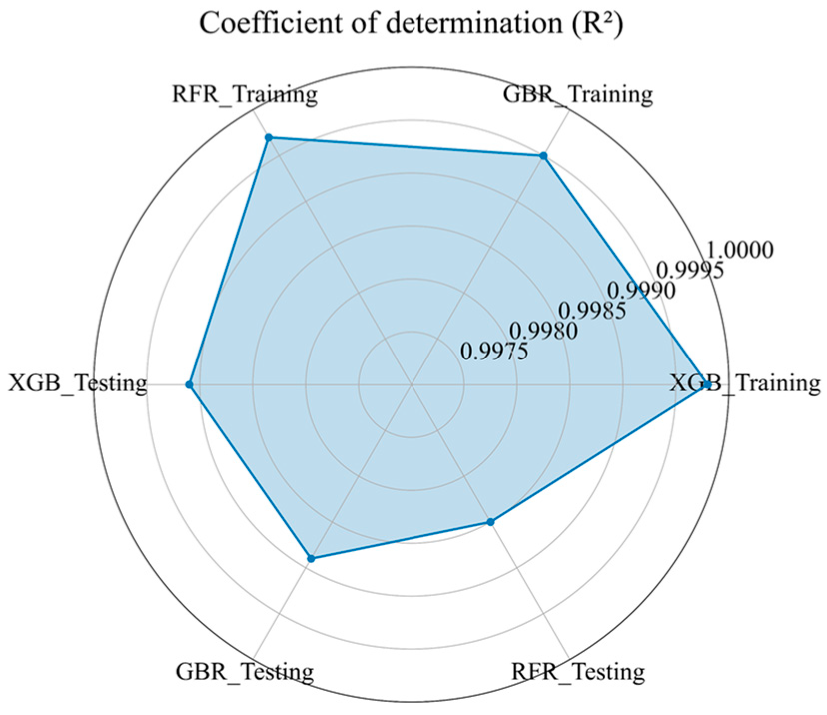
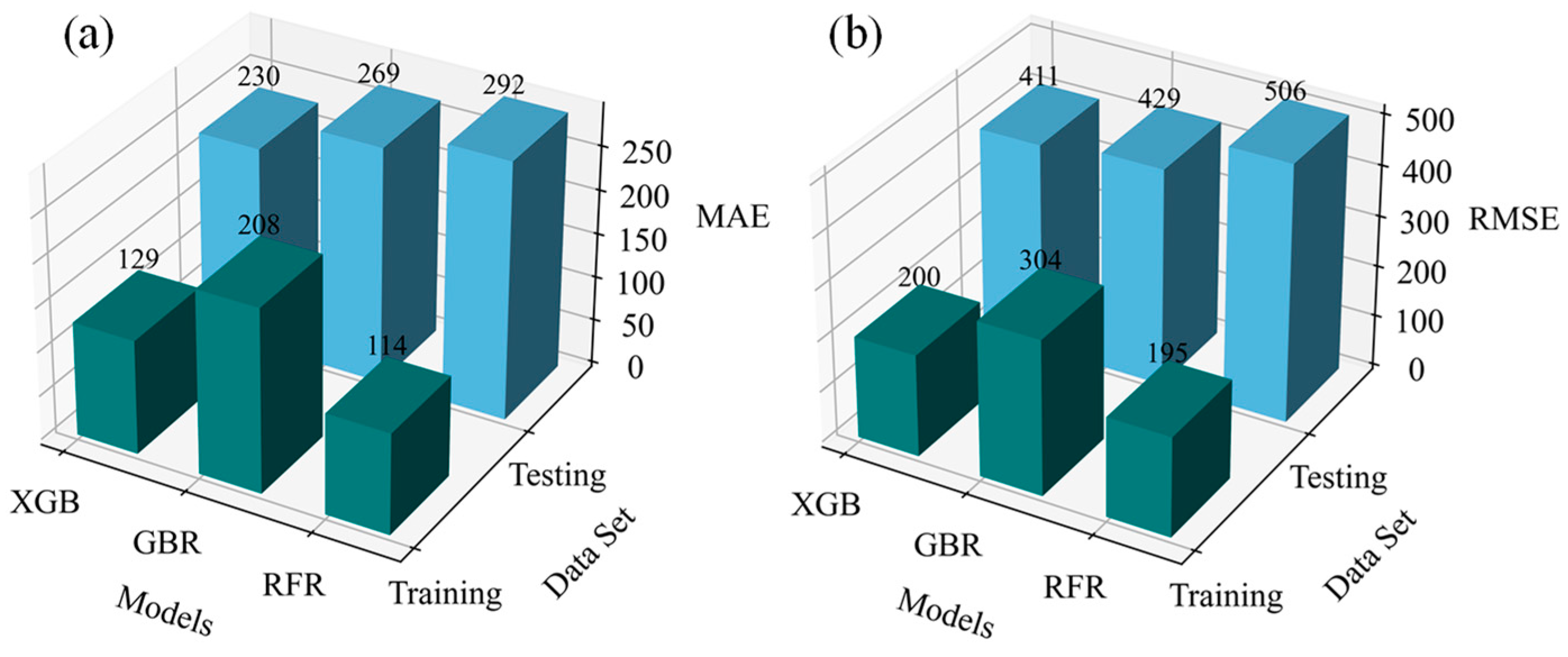
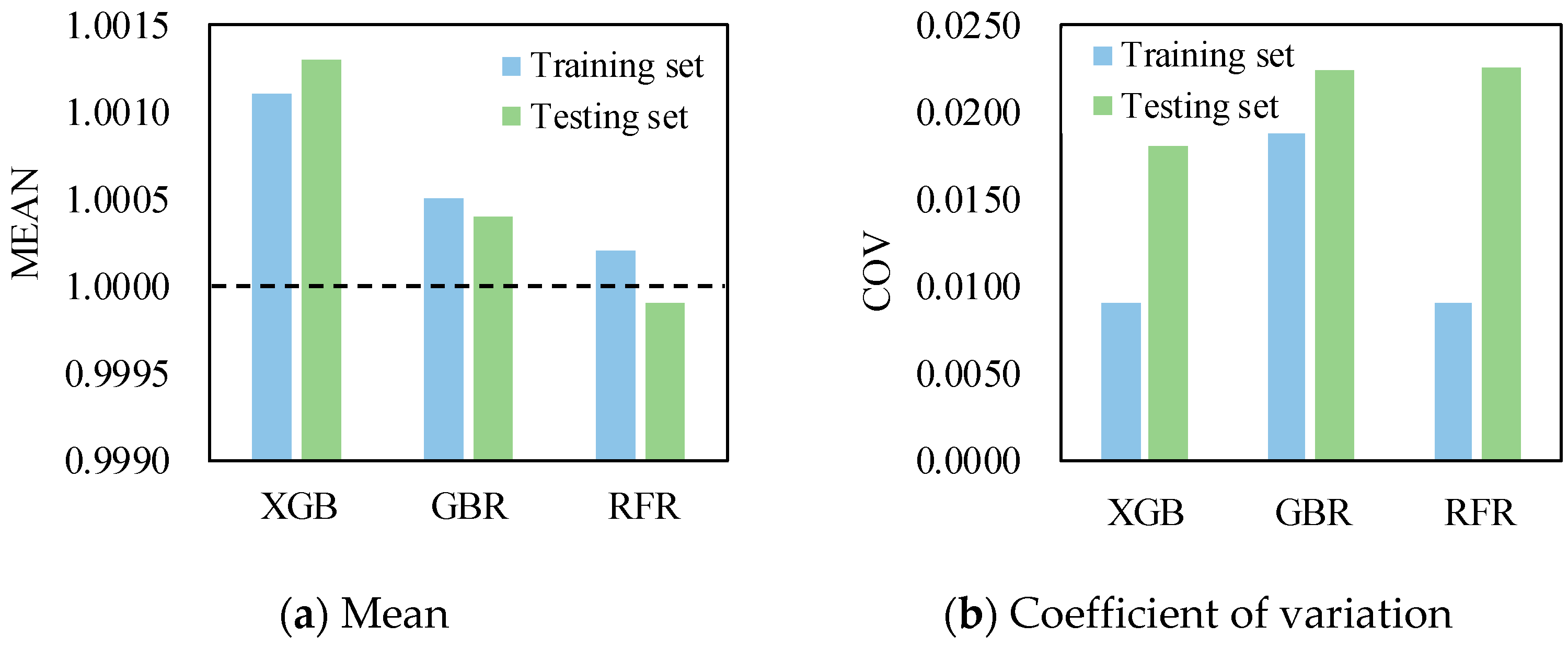
| Coefficient of Determination (R2) | Mean Absolute Error (MAE) | Root Mean Square Error (RMSE) | Mean (MEAN) | Coefficient of Variation (COV) | |
| Training Set /Testing Set | Training Set /Testing Set | Training Set /Testing Set | Training Set /Testing Set | Training Set /Testing Set | |
| XGB | 0.9998/0.9991 | 129/230 | 200/411 | 1.0011/1.0013 | 0.0091/0.0180 |
| GBR | 0.9995/0.9989 | 208/269 | 304/429 | 1.0005/1.0004 | 0.0188/0.0224 |
| RFR | 0.9997/0.9985 | 114/292 | 195/506 | 1.0002/0.9999 | 0.0091/0.0226 |
| ML Model | Percentage of Error (%) | ||||
|---|---|---|---|---|---|
| ≤0.5% | 0.5%~1% | 1%~5% | ≥5% | ||
| GBR | Training set | 28.2 | 21.9 | 47.6 | 2.4 |
| Testing set | 20.8 | 18.3 | 58.1 | 2.7 | |
| RFR | Training set | 55.3 | 24.7 | 19.9 | 0.1 |
| Testing set | 24.0 | 18.5 | 54.0 | 3.5 | |
| XGB | Training set | 100 | 0 | 0 | 0 |
| Testing set | 34.2 | 21.7 | 42.3 | 1.9 | |
| Ref. | Specimens | (kN) | (kN) | (kN) | (kN) | |||
|---|---|---|---|---|---|---|---|---|
| [10] | WST1-A | 3429 | 3326 | 0.97 | 3182 | 0.93 | 3327 | 0.97 |
| WST1-B | 3338 | 3326 | 1.00 | 3182 | 0.95 | 3327 | 1.00 | |
| WST2-A | 4162 | 3790 | 0.91 | 3549 | 0.85 | 3570 | 0.86 | |
| WST2-B | 4168 | 3760 | 0.90 | 3537 | 0.85 | 3570 | 0.86 | |
| WST3-A | 3929 | 3712 | 0.94 | 3586 | 0.91 | 3701 | 0.94 | |
| WST3-B | 4158 | 3686 | 0.89 | 3729 | 0.90 | 3960 | 0.95 | |
| WST4-A | 4492 | 4381 | 0.98 | 4361 | 0.97 | 4405 | 0.98 | |
| WST4-B | 5530 | 5013 | 0.91 | 5031 | 0.91 | 5048 | 0.91 | |
| WST5-A | 5620 | 5431 | 0.97 | 5158 | 0.92 | 5506 | 0.98 | |
| WST5-B | 5500 | 5484 | 1.00 | 5158 | 0.94 | 5629 | 1.02 | |
| WST6-A | 3240 | 3655 | 1.13 | 3341 | 1.03 | 3618 | 1.12 | |
| WST6-B | 2993 | 3655 | 1.22 | 3332 | 1.11 | 3681 | 1.23 | |
| WST7-A | 4826 | 5437 | 1.13 | 5457 | 1.13 | 5305 | 1.10 | |
| WST7-B | 4944 | 5437 | 1.10 | 5457 | 1.10 | 5305 | 1.07 | |
| WST8-A | 6521 | 6873 | 1.05 | 6345 | 0.97 | 6478 | 0.99 | |
| WST8-B | 6493 | 6838 | 1.05 | 6229 | 0.96 | 6478 | 1.00 | |
| WST9-A | 4203 | 4709 | 1.12 | 4832 | 1.15 | 4829 | 1.15 | |
| WST9-B | 4180 | 4705 | 1.13 | 4846 | 1.16 | 4892 | 1.17 | |
| WST10-A | 7201 | 6847 | 0.95 | 6484 | 0.90 | 7165 | 1.00 | |
| WST10-B | 6905 | 6465 | 0.94 | 6483 | 0.94 | 6120 | 0.89 | |
| WST11-A | 9065 | 8730 | 0.96 | 8160 | 0.90 | 9338 | 1.03 | |
| WST11-B | 8799 | 8851 | 1.01 | 9219 | 1.05 | 9338 | 1.06 | |
| [78] | CFRT1-A | 3429 | 3326 | 0.97 | 3182 | 0.93 | 3327 | 0.97 |
| CFRT1-B | 3338 | 3326 | 1.00 | 3182 | 0.95 | 3327 | 1.00 | |
| CFRT2-A | 4162 | 3790 | 0.91 | 3549 | 0.85 | 3570 | 0.86 | |
| CFRT2-B | 4168 | 3760 | 0.90 | 3549 | 0.85 | 3570 | 0.86 | |
| CFRT3-A | 3929 | 3712 | 0.94 | 3556 | 0.91 | 3701 | 0.94 | |
| CFRT3-B | 4158 | 3724 | 0.90 | 3556 | 0.86 | 3901 | 0.94 | |
| CFRT4-A | 4492 | 4434 | 0.99 | 4361 | 0.97 | 4345 | 0.97 | |
| CFRT4-B | 5530 | 5013 | 0.91 | 5031 | 0.91 | 5048 | 0.91 | |
| CFRT5-A | 5620 | 5431 | 0.97 | 5158 | 0.92 | 5629 | 1.00 | |
| CFRT5-B | 5500 | 5484 | 1.00 | 5158 | 0.94 | 5629 | 1.02 | |
| [79] | C1 | 1339 | 1256 | 0.94 | 1251 | 0.93 | 1158 | 0.86 |
| C2 | 1444 | 1465 | 1.01 | 1493 | 1.03 | 1372 | 0.95 | |
| C3 | 1755 | 1814 | 1.03 | 1787 | 1.02 | 1756 | 1.00 | |
| C4 | 1825 | 1822 | 1.00 | 1748 | 0.96 | 1840 | 1.01 | |
| C5 | 2125 | 2187 | 1.03 | 2190 | 1.03 | 2285 | 1.08 | |
| C6 | 2319 | 2904 | 1.25 | 2696 | 1.16 | 2976 | 1.28 | |
| C7 | 1623 | 1655 | 1.02 | 1618 | 1.00 | 1610 | 0.99 | |
| C8 | 1954 | 2145 | 1.10 | 2158 | 1.10 | 2043 | 1.05 | |
| [80] | RCFST-A-0 | 2094 | 2118 | 1.01 | 2028 | 0.97 | 1948 | 0.93 |
| [7] | RCFST-1 | 925 | 1047 | 1.13 | 947 | 1.02 | 1026 | 1.11 |
| RCFST-2 | 1215 | 1153 | 0.95 | 1357 | 1.12 | 1127 | 0.93 | |
| RCFST-3 | 1635 | 1902 | 1.16 | 1917 | 1.17 | 2047 | 1.25 | |
| RCFST-4 | 1658 | 1696 | 1.02 | 1566 | 0.94 | 1778 | 1.07 | |
| RCFST-5 | 2091 | 2342 | 1.12 | 2009 | 0.96 | 2231 | 1.07 | |
| [21] | RR-1-180-4 | 1755 | 1826 | 1.04 | 1885 | 1.07 | 1756 | 1.00 |
| RR-1-180-6 | 2319 | 2630 | 1.13 | 2608 | 1.12 | 2618 | 1.13 | |
| RR-0.5-180-6 | 1954 | 1997 | 1.02 | 2017 | 1.03 | 2038 | 1.04 | |
| RR-0.5-180-4 | 1623 | 1465 | 0.90 | 1493 | 0.92 | 1372 | 0.85 | |
| [81] | RRCFST-A-180-1 | 2026 | 2214 | 1.09 | 2338 | 1.15 | 2250 | 1.11 |
| RRCFST-A-180-2 | 1915 | 2214 | 1.16 | 2334 | 1.22 | 2316 | 1.21 | |
| RRCFST-C-180-1 | 1574 | 1655 | 1.05 | 1761 | 1.12 | 1704 | 1.08 | |
| [82] | PY1-180-e0-fy235 | 1780 | 1720 | 0.97 | 1735 | 0.97 | 1736 | 0.98 |
| PY1-180-fy345 | 2100 | 1928 | 0.92 | 2076 | 0.99 | 2036 | 0.97 | |
| PYRE1-180-fy345 | 2060 | 1928 | 0.94 | 2076 | 1.01 | 2036 | 0.99 | |
| [83] | RCC1-4-180 | 1755 | 1814 | 1.03 | 1729 | 0.99 | 1756 | 1.00 |
| RCC1-6-180 | 2319 | 2523 | 1.09 | 2529 | 1.09 | 2503 | 1.08 | |
| RCC0.5-4-180 | 1623 | 1459 | 0.90 | 1251 | 0.77 | 1351 | 0.83 | |
| RCC0.5-6-180 | 1954 | 1904 | 0.97 | 1823 | 0.93 | 1865 | 0.95 | |
| Mean | 1.01 | 0.99 | 1.01 | |||||
| Standard deviation | 0.09 | 0.10 | 0.10 |
Disclaimer/Publisher’s Note: The statements, opinions and data contained in all publications are solely those of the individual author(s) and contributor(s) and not of MDPI and/or the editor(s). MDPI and/or the editor(s) disclaim responsibility for any injury to people or property resulting from any ideas, methods, instructions or products referred to in the content. |
© 2024 by the authors. Licensee MDPI, Basel, Switzerland. This article is an open access article distributed under the terms and conditions of the Creative Commons Attribution (CC BY) license (https://creativecommons.org/licenses/by/4.0/).
Share and Cite
Chen, D.; Fan, Y.; Zha, X. Machine Learning-Based Strength Prediction of Round-Ended Concrete-Filled Steel Tube. Buildings 2024, 14, 3244. https://doi.org/10.3390/buildings14103244
Chen D, Fan Y, Zha X. Machine Learning-Based Strength Prediction of Round-Ended Concrete-Filled Steel Tube. Buildings. 2024; 14(10):3244. https://doi.org/10.3390/buildings14103244
Chicago/Turabian StyleChen, Dejing, Youhua Fan, and Xiaoxiong Zha. 2024. "Machine Learning-Based Strength Prediction of Round-Ended Concrete-Filled Steel Tube" Buildings 14, no. 10: 3244. https://doi.org/10.3390/buildings14103244
APA StyleChen, D., Fan, Y., & Zha, X. (2024). Machine Learning-Based Strength Prediction of Round-Ended Concrete-Filled Steel Tube. Buildings, 14(10), 3244. https://doi.org/10.3390/buildings14103244