Investigating of Spatiotemporal Correlation between Urban Spatial Form and Urban Ecological Resilience: A Case Study of the City Cluster in the Yangzi River Midstream, China

Abstract

The anthropogenic disturbance caused by irrational urbanization impacts the ecological security of cities. The study of the relationship between urban spatial form (USF) and urban ecological resilience (UER) can offer guidance for sustainable urban development. We select the UER evaluation indexes and construct a DRSIR model based on the causal relationship among the natural, social, and economic dimensions of cities. We also carried out empirical research on the impact of USF on UER in the city cluster located in the Yangtze River midstream (YRM) through the geographical and temporal weighted regression (GTWR) model and geographical detector for four time cross-sections: 2005, 2010, 2015, and 2020. The following findings were obtained: (1) The computing results for UERIs of cities in the YRM noticeably and consistently increased during the study period, exhibiting a spatial distribution pattern with high values in the southeast, second-highest in the northwest, and low values in the center. (2) The regression coefficients of USFIs and UERIs displayed significant spatial and temporal variations in the YRM during the study period. (3) CA, AWMPFD, PD, and AI showed a positive correlation with UERIs, while PD exhibited a negative correlation with UERIs. (4) LPI and AI emerged as the primary drivers of spatial heterogeneity in UERIs, and the interaction between these two factors significantly enhanced their impact on UERIs compared to individual influencing factors. Exploring the correlation between UER and USF can be utilized to provide urban management recommendations that are suitable for the level of urban development, which will contribute to the achievement of sustainable development in the YRM.

1. Introduction

In recent years, the problem of global cities’ ecological security has been prevalent. On the one hand, cities face the impact of natural disasters such as climate change [1] and earthquakes [2]. On the other hand, as urbanization and industrialization advance rapidly, the negative effects of man-made disturbances such as disease transmission [3] and environmental pollution [4] are becoming increasingly severe, and the impact of slow-onset disturbances such as irrational urbanization [5] on urban ecological problems is becoming increasingly significant. To cope with the growing pressure on ecosystems, the International Council for Sustainable Regional Development (ICLEI) proposed the topic of “urban resilience” for the first time in 2002 [6]. The United Nations Office for Disaster Risk Reduction (UNDRR)’s “Top Ten Indicators of Urban Resilience” includes “Protecting Urban Ecosystems and Natural Barriers”, signaling the importance of resilience to ecosystems [7]. Urban ecological resilience (UER) describes the response of urban ecosystems to environmental perturbations and measures the ability of ecosystems to adapt to and recover quickly from external disturbances [8,9,10]. Nowadays, cities around the world are experiencing spatial expansion and drastic changes in spatial form as a result of rapid urbanization, posing great challenges to UER. Therefore, from the perspective of maintaining urban ecological security, it is necessary to study the association between urban spatial form (USF) and UER.

In the field of UER measurement research, numerous studies have been conducted to establish a foundation for the quantitative analysis of UER. Currently, two primary models are employed to measure UER: the “resistance–adaptation–recovery” model, which is based on ecological resilience characteristics [11], and the “driver–pressure–state–impact–response” (DPSIR) model. The DPSIR model includes the PSR model proposed by the Organization for Economic Co-operation and Development (OECD) and the United Nations Environment Programme (UNEP) [12,13], the “Drive–State–Response” (DSR) model, the “Pressure–State–Response–Pattern” (PSRP) framework proposed by the United Nations Conference on Sustainable Development (UNCSD) [14], and the “Drive–Pressure–State–Exposure–Effect–Action” DPSEEA model [15]. While the “Resistance–Adapt–Recovery” (RAR) model focuses on the relationship between urban economic, social, and ecological indicators that collectively contribute to ecological resilience, it still relies on individual network elements for measurement. Moreover, its scope and boundaries are too narrow to encompass the full breadth and depth of UER. In contrast, the DPSIR framework, rooted in an in-depth understanding and analysis of the complex causal linkages among urban economic, social, and ecological systems, utilizes a modeling approach to reflect the causal connections between urban ecological pressures and responses, thereby assessing UER effectively. This perspective provides a robust foundation for evaluating UER from a human–natural ecosystem standpoint.

In the study of factors influencing UER, Lyu et al. used the STIRPAT model to select the factors influencing ecological resilience in the Yangtze River Delta region from the population, economic, and technological factors and found that the economic factors had a positive promoting effect on urban ecological resilience, and the population, technological, and land factors had an inverse inhibitory effect on urban ecological resilience [16]. Wang et al. measured the impacts of urbanization on UERE in the Pearl River Delta region and found that the urbanization level and ecological resilience slipped from basic coordination to basic dysfunction [17]. Zhou et al. analyzed the impact of smart city development on ecological resilience and found that the construction of smart cities had no significant impact on ecological resilience [18]. Although there have been studies discussing the influencing factors of UER, there are few studies discussing UER from the perspective of USF.

USF affects the agglomeration and size effects of regional economic development by changing the scale and type of land use. It also has implications for the level of urban economic returns [19,20], the construction scale and layout of hospitals and schools [21], as well as the development of road transport systems and urban pipeline networks [22]. These factors, in turn, significantly impact the ecological resilience of cities [23,24]. Currently, numerous scholars have conducted research on the environmental effects of USF [25], and explored the relationship between USF and aspects such as carbon emissions [26,27], carbon balance [28], and heat islands [29]. However, there remains a need for further investigation into the temporal and spatial relationships and interactions between urban spatial patterns and ecological resilience.

Since the reform and opening up, China’s urbanized population has risen from 172.45 million in 1978 to 920.71 million in 2022, and the urbanization rate of the resident population has risen from 17.92% in 1978 to 65.2% in 2022 [30], making China’s urbanization a world-renowned achievement. However, urban ecosystems are also facing disturbances caused by excessive human development [31,32]. Against this background, the construction of ecological civilization has attracted great attention from the Chinese government [33]. The city cluster in the midstream of the Yangtze River (YRM) serves as the core area for the construction of ecological civilization in the Yangtze River Economic Belt and plays a crucial role in maintaining the ecological security pattern of the basin [34]. Over the past decade, it emerged as a significant new economic growth pole in China, with a GDP of 11.1 trillion yuan in 2020, accounting for 9.3% of the country’s total GDP. While there has been rapid socio-economic development [35], the development gap between cities in the region has been widening, and the ecosystem has been subject to varying degrees of anthropogenic disturbance. Therefore, these cities in the YRM characterized by differing levels of development and ecological disturbance are typical examples and hold research value in the fields of USF and UER.

This paper aims to investigate the impact of USF on UER, enhance the existing ecological resilience measurement methods by considering urban natural, social, and economic dimensions, and analyze USF using selected landscape pattern metrics. Furthermore, we analyzed the impact of USF on UER in the YRM using the geographical and temporal weighted regression (GTWR) model and geographical detector for four different time points: 2005, 2010, 2015, and 2020. The results of this study are expected to provide essential support for optimizing urban morphology, ensuring ecological environmental security, and promoting sustainable urban development.

2. Materials and Methods

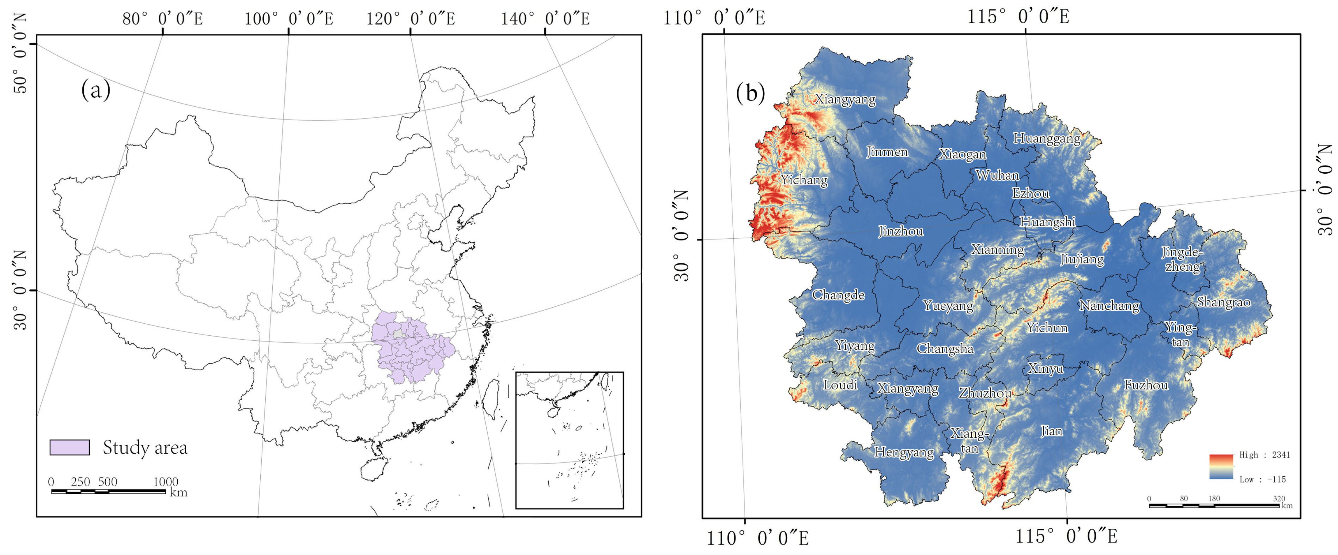
2.1. Study Area

The city cluster in the YRM is located in central China, encompassing 31 cities, including 28 prefecture-level cities and 3 county-level cities in Hubei, Hunan, and Jiangxi Provinces. The total area of this city cluster is 32.61 km². Considering the city level and data accessibility, we chose 28 prefecture-level cities as the study area. The study area is located at ${110}^{\circ }{15}^{\prime }$ E–${117}^{\circ }{97}^{\prime }$ E, ${27}^{\circ }{12}^{\prime }$ N–${32}^{\circ }{37}^{\prime }$ N (Figure 1).

2.2. Data

The natural geographic data required for this study included data on urban construction land, digital elevation data (DEM), and land use data. The socio-economic data consisted of information on the number of green inventions and other relevant statistical data. Specific data sources and descriptions can be found in

Table 1. Data source and descriptions.

Data Name	Data Layout	Data Sources	Data Usage
Urban construction land data	Raster data with resolution of 30 m	Resource and Environment Science and Data Center (http://www.resdc.cn, accessed on 2 August 2023)	Basic data for calculating USFIs
Digital elevation model (DEM) data	Raster data with resolution of 30 m	Geospatial data cloud system of Computer Network Information Center, Chinese Academy of Sciences (http://www.gscloud.cn), accessed on 2 August 2023	Basic data for calculating city slope, and slope direction
Land use data	Excel	Land survey results sharing application service platform of Ministry of Natural Resources (https://gtdc.mnr.gov.cn), accessed on 7 August 2023	The factors of UERIs
Social and economic data	Excel	Statistical Yearbook of Hubei, Hunan, Jiangxi Province and Cities	The factors of UERIs
Number of green inventions	Excel	China National Intellectual Property Database (https://www.cnipa.gov.cn), accessed on 9 August 2023	The factor of UERIs

.

2.3. Urban Spatial Form (USF)

2.3.1. Landscape Pattern Metrics

USF is typically assessed using landscape pattern metrics in previous studies, and two methods are employed for selecting these indices: (1) subjective empirical method: combining specific index information with practical significance, scholars select indices suitable for the study’s purpose. (2) Empirical validation method: scholars select multiple indices, assess their covariance, and then refine the selection to determine the final set of indices. In our study, we chose ten indicators like class area (CA), patch destiny (PD), largest patch index (LPI), edge destiny (ED), landscape shape index (LSI), mean patch size (MPS), euclidean average nearest neighbour distance (ENN_MN), patch cohesion index (COHESION), aggregation index (AI), and area-weighted mean patch fractal dimension (AWMPFD) to be measured in Fragstats 4.2, and then selected five indicators from them through Spearman’s correlation coefficient and factor analysis (

Table A1. Landscape pattern metrics, formulas, and instructions [49].

Landscape Pattern Metric	Formula	Instruction
CA	${\displaystyle \sum _{i=1}^n}{a}_{ij}(1/\mathrm{10,000})$	$a_{ij}$ = area ($m^2$) of patch $ij$.
PD	$\frac{n_i}{A}\left(\mathrm{10,000}\right)\left(100\right)$	$n_i$ = number of patches in the landscape of patch type (class) i. A = total landscape area ($m^2$).
LPI	$\frac{max\left({a_i}_j\right)}{A}\left(100\right)$	$a_{ij}$ = area ($m^2$) of patch $ij$. A = total landscape area ($m^2$).
ED	$\left(\mathrm{10,000}\right){\displaystyle \sum _{i=1}^n}{e}_i/A$	$e_{ij}$ = total length (m) of edge in landscape involving patch type (class) i includes landscape boundary and background segments involving patch type i. A = total landscape area ($m^2$).
LSI	$$\frac{0.25{\displaystyle \sum _{i=1}^n}{\displaystyle \sum _{j=1}^m}{e}_{ij}}{\sqrt{A}}$$	$e_i$ = total length (m) of edge in landscape involving patch type (class) i includes landscape boundary and background segments involving patch type i. A = total landscape area ($m^2$).
MPS	$\frac{{\displaystyle \sum _{i=1}^n}{a_i}_j}{n_i}$	$a_{ij}$ = area ($m^2$) of patch $ij$. $n_i$ = number of patches in the landscape of patch type (class) i.
ENN_MN	$\frac{{\displaystyle \sum _{j=1}^n}{h}_{ji}}{n}$	$h_{ij}$ = distance (m) from patch $ij$ to nearest neighboring patch of the same type (class), based on patch edge-to-edge distance, computed from cell center to cell center.
COHESION	$\left[1-\frac{{\displaystyle \sum _{j=1}^m}{p}_{ij}}{{\displaystyle \sum _{j=1}^m}{p}_{ij}\sqrt{a_{ij}}}\right]{\left[1-\frac{1}{\sqrt{A}}\right]}^{-1}\times 100$	$p_{ij}$ = perimeter of patch $ij$ in terms of number of cell surfaces. $a_{ij}$ = area of patch $ij$ in terms of number of cells. Z = total number of cells in the landscape.
AI	$\left[\frac{g_{ij}}{max\to g_{ij}}\right]\left(100\right)$	$p_{ij}$ = number of like adjacencies (joins) between pixels of patch type (class) i based on the single-count method. Max$\to g_{ij}$ = maximum number of like adjacencies (joins) between pixels of patch type (class) i based on the single-count method.
AWMPFD	${\displaystyle \sum _{i=1}^n}\left[\frac{2ln\left(0.25p_{ij}\right)}{ln{a}_{ij}}\right]\left[\frac{a_{ij}}{{\displaystyle \sum _{j=1}^n}{a}_{ij}}\right]$	$p_{ij}$ = perimeter (m) of patch $ij$. $a_{ij}$ = area ($m^2$) of patch $ij$.

,

Table 2. Results of Spearman’s correlation coefficient.

	CA	PD	LPI	ED	LSI	MPS	ENN_MN	COHESION	AI	AWMPFD
CA	1.000
PD	−0.112	1.000
LPI	−0.206	−0.126	1.000
ED	−0.461	0.565	−0.352	1.000
LSI	0.785	0.181	0.131	0.065	1.000
MPS	0.101	−0.999	0.170	−0.567	−0.190	1.000
ENN_MN	0.026	−0.010	−0.282	−0.277	0.054	0.015	1.000
COHESION	−0.168	−0.393	0.760	−0.051	−0.266	0.392	−0.459	1.000
AI	−0.588	−0.394	0.427	−0.154	−0.825	0.400	−0.221	0.569	1.000
AWMPFD	0.316	0.005	0.336	0.285	0.486	−0.013	−0.506	0.584	−0.226	1.000

and

Table 3. Results of factor analysis.

	PC1	PC2	PC3
Eigenvalue	3.587	2.543	1.816
Variability (%)	35.875	25.427	18.156
Cumulative (%)	35.875	61.302	79.458
Factor loadings
CA	0.843	0.387	−0.152
PD	0.068	−0.864	−0.112
LPI	−0.345	0.264	0.702
ED	−0.210	−0.643	0.169
ENN_MN	0.110	0.328	−0.565
AI	−0.892	0.218	0.243
AWMPFD	0.329	−0.167	0.879

).

2.3.2. Spearman Correlation

We employed Spearman correlation coefficient to test for independence between the indicators. The significance of the correlation coefficients was assessed using a two-tailed t-test with significance levels of 0.05 and 0.01. A correlation coefficient greater than 0.7 indicates a strong degree of independence between the data [36]. The formula is as follows:

$$r_i=1-\frac{6\sum {d_i}^2}{n(n^2-1)}$$

(1)

where n represents the number of rank pairs of the x and y variables, which corresponds to the sample size. $d_i$ is the difference between the ranks of the same pair ($i=1,2,...,n$). In this study, we logarithmized the indices CA, LPI, ED, MPS, ENN_MN, COHESION, and AI. The strength of the association between the bivariate variables was analyzed using Spearman correlation to account for data covariance. For combinations with correlation coefficients greater than 0.7, one of the indicators was excluded from further analysis. The Spearman correlation coefficients revealed strong correlations between some of the landscape pattern metrics. CA showed a strong positive correlation with LSI, indicating that larger cities tend to have more complex shapes. PD exhibited a strong negative correlation with MPS, suggesting that more centralized cities have less fragmented urban morphology. LPI demonstrated a strong positive correlation with COHESION, indicating that greater urban centrality is associated with better connectivity between patches. After excluding LSI, MPS, and COHESION, the correlation coefficients of the remaining seven indicators were all below 0.7, indicating their independence from each other (Table 2).

2.3.3. Factor Analysis

Factor analysis is employed to describe the relationship between numerous indicators or factors and a smaller number of underlying factors [37]. In this study, we used factor analysis to obtain the factor loading matrix |A| and factor score matrix |S|. These matrices were used to categorize landscape indices and analyze the extent to which each index contributed to each category of the common factor. The formula is as follows:

$$\left|\mathrm{X}\right|=\left|\mathrm{A}\right|\times \left|\mathrm{F}\right|+\left|\mathrm{E}\right|$$

(2)

where |X| represents the original vector of variables, |A| is the loading matrix of the common factors, |F| is the vector of common factors, and |E| represents the effect of the common factors on the variance of the data, which is negligible. Factor scores are also calculated for |F| to illustrate the contribution of the variables to the common factors. In this study, we extracted three factors through principal component analysis based on eigenvalues greater than 1. These three factors collectively explained 79.458% of the total variance. This meant that a substantial amount of the original information was retained, and the representation of the factors was ideal and held research significance. According to the results of the rotated component matrix, PC1 explains the largest proportion of variance (35.875%) with an eigenvalue of 3.587. The key landscape metrics in PC1 are CA (−0.843) and AI (0.892), indicating that PC1 represents the scale of the patches and the degree of connectivity. In PC2, pd (0.864) is the representative variable, and PC2 can be associated with the density of the patches. PC3 is characterized by LPI (0.702) and AWMPFD (0.879), representing the centrality and shape complexity of patches. LPI, ED, and ENN_MN did not exhibit a clear representation in the first three principal components (Table 3). As a result, we chose five indices (CA, PD, LPI, AI, and AWMPFD) to represent USF. Three cities with spatial form and landscape metrics in the midstream of the Yangtze River are shown in Figure 2.

2.4. Urban Ecological Resilience (UER) Calculation Method

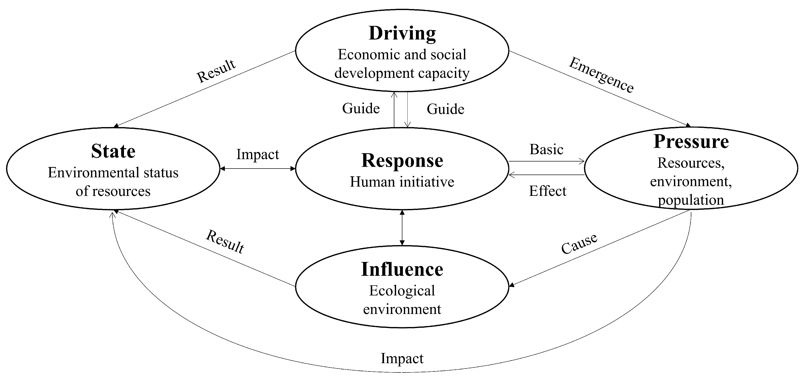
2.4.1. Evaluate Urban Ecosystem Resilience in the DPSIR Framework

UER places emphasis on the ability of urban ecosystems to resist, adapt to, or recover from external shocks. The DPSIR model is based on the cause-and-effect relationship of driver–pressure–state–impact–response, effectively reflecting the system’s causal relationships. The DPSIR model is a suitable method for evaluating the ecological resilience of cities, as it integrates elements related to resources, development, environment, and human health, effectively reflecting the causal relationships within the system. In the DPSIR model, the term ‘driver’ refers to the social and economic factors that drive changes in ecological resilience. ‘Pressure’ pertains to the impact of human production, construction, and other activities on the natural environment. ‘State’ describes the condition of the ecological environment in the context of the aforementioned driving forces and pressures. ‘Impact’ indicates the influence of the ecological environment on human health and socio-economic structure. ‘Response’ encompasses the positive measures taken by humans to promote the growth of ecological resilience (

Table 4. UER evaluation indicator system in the DPSIR framework.

Target	Subsystem	Factor	Indicator	Indicator Attribute
UER	Driver D	Social motivation	Population Urbanisation Rate	−
		Economic motivation	GDP per capita	+
			Average income of employees	+
			Total retail sales of consumer goods	+
	Pressure P	Social pressure	Population density	−
			Natural growth rate	−
		Resource demand pressure	Total water supply	−
			Urban construction land area	−
		Environmental pressure	Industrial Sulphur Dioxide Emission	−
			Industrial wastewater discharge	−
	State S	Ecological quality level	Greening coverage rate of built−up area	+
			Cultivated land area	+
	Impact I	Ecological Impact	Grassland area	+
			Woodland area	+
		Social Impact Index	Number of labour force	+
	Response R	Social−Economic Input	Number of green inventions	+
			Share of tertiary industry in GDP	+
		Pollution Control	Removal of Industrial Smoke and Dust	+
			Harmless treatment rate of domestic waste	+

).

2.4.2. Entropy Weight Method

• Standardization of data.
  For positive indicators:

  $$y_{ij}=\frac{x_{ij}-min{x}_i}{max{x}_i-min{x}_i}$$

  (3)
  For negative indicators:

  $$y_{ij}=\frac{max{x}_i-x_{ij}}{max{x}_i-min{x}_i}$$

  (4)

  where $y_{ij}$ is the standardized value of the data; $x_{ij}$ refers to the original indicator; max $x_i$ and min $x_j$ denote the maximum and minimum values within indicator J.
• Calculation of indicator weights.

  $$H_j=-k\sum _{i=1}^n{f}_{ij}{\mathrm{lnf}}_{ij}$$

  (5)

  where $H_j$ is the entropy value of the $j_{th}$ indicator, $k=1/lnm$, $f_{ij}=y_{ij}/{\displaystyle \sum _{i=1}^n}{y}_{ij}$ [38].

2.4.3. Reliability and Validity of Indicator System

Partial Least Squares Structural Equation Modeling (PLS-SEM) is widely used to assess the reliability and validity of a set of indicators [39]. Generally, Cronbach’s alpha should be greater than 0.6, and composite reliability (CR) should exceed 0.7 [40]. The average variance extracted (AVE) indicates the convergent validity of the indicators, and AVE should be greater than 0.5 [41]. Additionally, the square root of AVE should be higher than its correlation with any other latent variable.

Table 5. Reliability and validity of DPSIR framework.

	Cronbach’s Alpha	CR	AVE
D	0.918	0.941	0.801
P	0.859	0.857	0.677
S	0.767	0.719	0.598
I	0.638	0.784	0.786
R	0.813	0.801	0.585

and

Table 6. Discriminant validity.

	D	P	S	I	R
D	0.895
P	0.666	0.823
S	0.722	0.779	0.773
I	0.867	0.647	0.770	0.887
R	0.291	0.148	0.034	0.289	0.765

revealed significant differences among the five components of UER.

$$C{R}_i=\frac{({\displaystyle \sum _{h=1}^{P_j}}{\lambda }_{jh}{)}^2}{({\displaystyle \sum _{h=1}^{P_j}}{\lambda }_{jh}{)}^2+({\displaystyle \sum _{h=1}^{P_j}}{\theta }_{jh}{)}^2}$$

(6)

where ${\lambda }_{jh}$ is the weight of index h in component j, and ${\theta }_{jh}$ is the measurement error of index h in component j. In this study, each component’s Cronbach’s alpha exceeded 0.6, and each component’s CR exceeded 0.7 (Table 5), indicating that the indicator system of UER is highly reliable.

$$AV{E}_i=\frac{{\displaystyle \sum _{h=1}^{P_i}}{{\lambda }_{jh}}^2}{{\displaystyle \sum _{h=1}^{P_i}}{{\lambda }_{jh}}^2+{\displaystyle \sum _{h=1}^{P_i}}{{\theta }_{jh}}^2}$$

(7)

where ${\lambda }_{jh}$ represents the weight of indicator h for node j, and ${\theta }_{jh}$ is the measurement error of indicator h in node j. In this study, AVE of each variable exceeds 0.5 (Table 6), indicating that the indicator dimensions have convergent validity.

2.5. Geographical and Temporal Weighted Regression (GTWR) Model

The traditional regression model and geographical weighted regression (GWR) model do not account for spatial heterogeneity and temporal elements [42]. Therefore, we opted for a GTWR model to consider the influence of spatiotemporal effects on the explanatory variables. This choice allows us to analyze the spatiotemporal heterogeneous characteristics of the impact of different USFIs on UERIs. The model is as follows:

$$y_i={\beta }_0(u_i,v_i,t_i)+\sum _{k=1}^k{\beta }_k(u_i,v_i,t_i)x_{ik}+{\epsilon }_i$$

(8)

where $t_1$ represents the time of the study. ${\beta }_0(u_i,v_i,t_i)$ represents the spatiotemporal intercept for observation i and ${\beta }_k(u_i,v_i,t_i)$ is the coefficient of the kth independent variable at observation i.

$$VI{F}_j=\frac{1}{1-{R_j}^2}$$

(9)

where $r_j^2$ is the coefficient in a multiple regression of explanatory variables. In this study, VIF of all explanatory variables was less than 5 and the mean VIF was less than 5 (

Table 7. Results of a multicollinearity test based on OLS estimation.

	${\mathit{X}}_1$	${\mathit{X}}_2$	${\mathit{X}}_3$	${\mathit{X}}_4$	${\mathit{X}}_5$
VIF	3.255	2.190	2.717	2.717	1.236
1/VIF	0.307	0.457	0.368	0.368	0.809
Mean VIF			2.423

), which indicates that there is no multicollinearity, and it met the requirements of GTWR model estimation.

2.6. Geographical Detector

The geographical detector is a statistical method used to detect spatial dissimilarities and reveal the driving forces behind them. Additionally, it is immune to covariance and can disregard correlations between factors [43]. The geographical detector is employed to quantitatively explain the extent to which USFIs affect UERIs in the YRM. It also analyzes the effects of the interactions of various USFIs.

Factor Detection. To understand the degree to which the factor X USFIs explains the dependent variable Y UERIs, the formula is as follows:

$$\mathrm{q}=1-\frac{1}{N{\sigma }^2}\sum _{\mathrm{h}=1}^L{N}_h{{\sigma }_h}^2$$

(10)

where q is the degree of interpretation of factor X on UER divergence, and the range of values is [0, 1]; a larger value of q indicates a greater impact of the factor on UER; $h=1,2,\dots ,L$; L is the number of factor X classification; $N_h$ and N are the number of samples of the $h_{th}$ class and total numbers of samples in the region; ${\sigma }_h$, $\sigma$ are the variance of the $h_{th}$ class of factor X and total variance in the region.

Interaction Detection. Discriminating the difference in explanatory power when factors Xi and Xj act together relative to when they act alone.

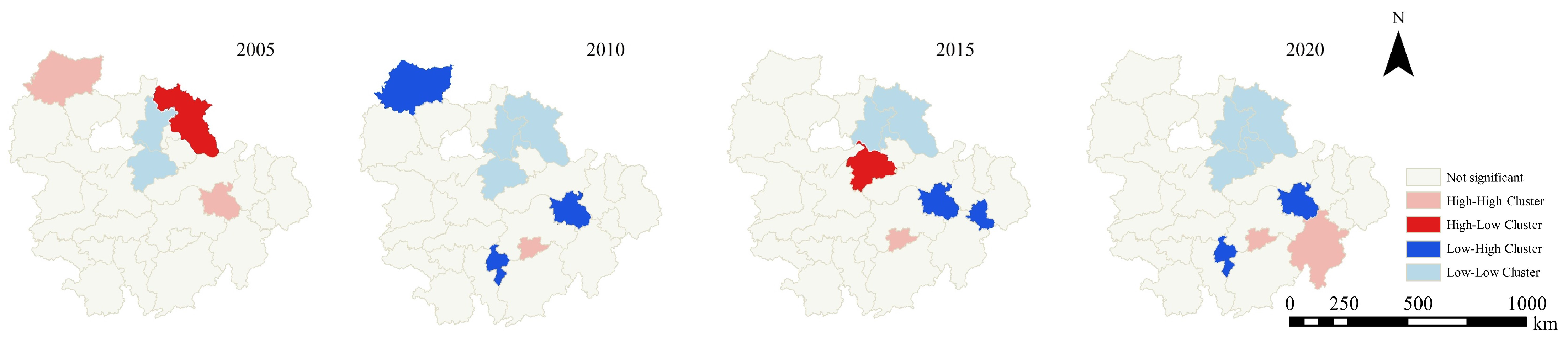
2.7. Spatial Autocorrelation Analysis

Spatial autocorrelation analysis is a spatial statistical method used to examine the correlation of attributes in neighboring locations, and it is widely employed in spatial correlation studies [44]. In our analysis, we examined the distribution characteristics of UER, such as spatial discreteness or aggregation. Spatial autocorrelation analysis encompasses both global spatial autocorrelation (Moran’s I index) and local spatial autocorrelation (LISA index). We used Moran’s I index to assess the spatial agglomeration pattern of UERIs. Additionally, we utilized the LISA index to characterize the correlation between local elements and neighboring units. It allowed us to test whether there is a phenomenon of agglomeration of similar or dissimilar attribute values in the local area. The results of the LISA analysis are categorized as LL-type (low–low agglomeration), HH-type (high–high agglomeration), HL-type (low-value surrounded by high-value aggregation), and LH-type (high-value surrounded by low-value aggregation). The local spatial autocorrelation coefficient of ecological resilience in cities in the YRM can be expressed as follows:

$$\mathrm{Ł}\mathrm{i}=\frac{(x_i-\overline{x})}{S^2}\sum _{j=i}^n{w}_{ij}{z}_{ij}$$

(11)

In the formula, Łi is the $LISA$ index of the city, $S^2=\frac{1}{\mathrm{n}}\sum {(Z\mathrm{i}-\overline{Z})}^2$, $w_{ij}$ is the spatial weight value. $Li>$ 0 includes high–high and low–low areas, $Li<$ 0 includes low-high and high-low areas.

3. Results

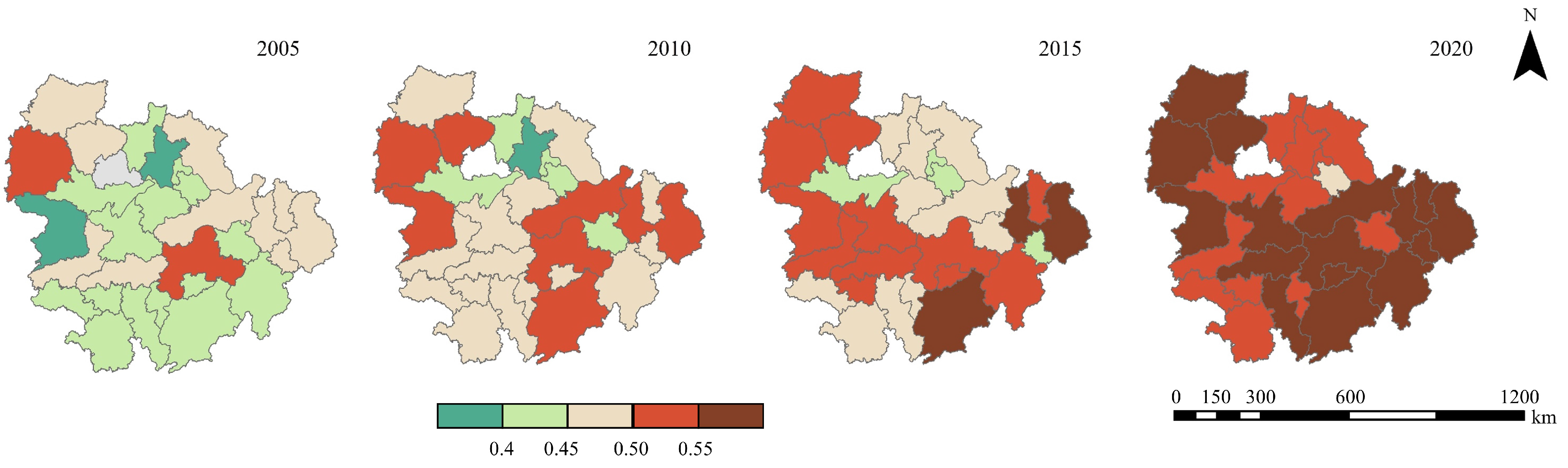
3.1. Spatial and Temporal Characteristics of UERIs

UERIs were categorized into five levels, ranging from low to high (I low, II lower, III medium, IV higher, and V high resilience), with thresholds set at 0.30, 0.40, 0.50, and 0.60, based on values defined in previous literature. Over the study period, UERIs showed clear growth trends (Figure 3), with high levels observed in the southeast, followed by the northwest, and low levels in the central part of the spatial distribution (Figure 4). Cities with UERI level V were primarily located in Jiangxi Province, while UERI level I cities were mainly situated in central cities like Wuhan and Changsha, as well as their surrounding areas. From 2005 to 2020, the proportion of UERI level IV cities increased from 7% in 2005 to 43% in 2020, while the proportion of UERI level II cities decreased from 54% in 2005 to 0% in 2020.

We determined the types of ecological resilience agglomeration and spatial layout of cities through spatial autocorrelation analysis (LISA). From 2005 to 2020, areas with “low–low” were primarily found in Wuhan and its surrounding cities, such as Xianning and Huanggang. In 2005, Xiangyang and Nanchang were “high–high” cities. From 2010 to 2020, Xinyu was the “high–high” city, and in 2020, Fuzhou was added to the list of “high–high” cities. In 2010 and 2020, the areas with UERI “low–high” were in Nanchang and Pingxiang, and in Nanchang and Yingtan in 2015. This indicated that UERIs in Nanchang were at a low level during the same period from 2010 to 2020 (Figure 5).

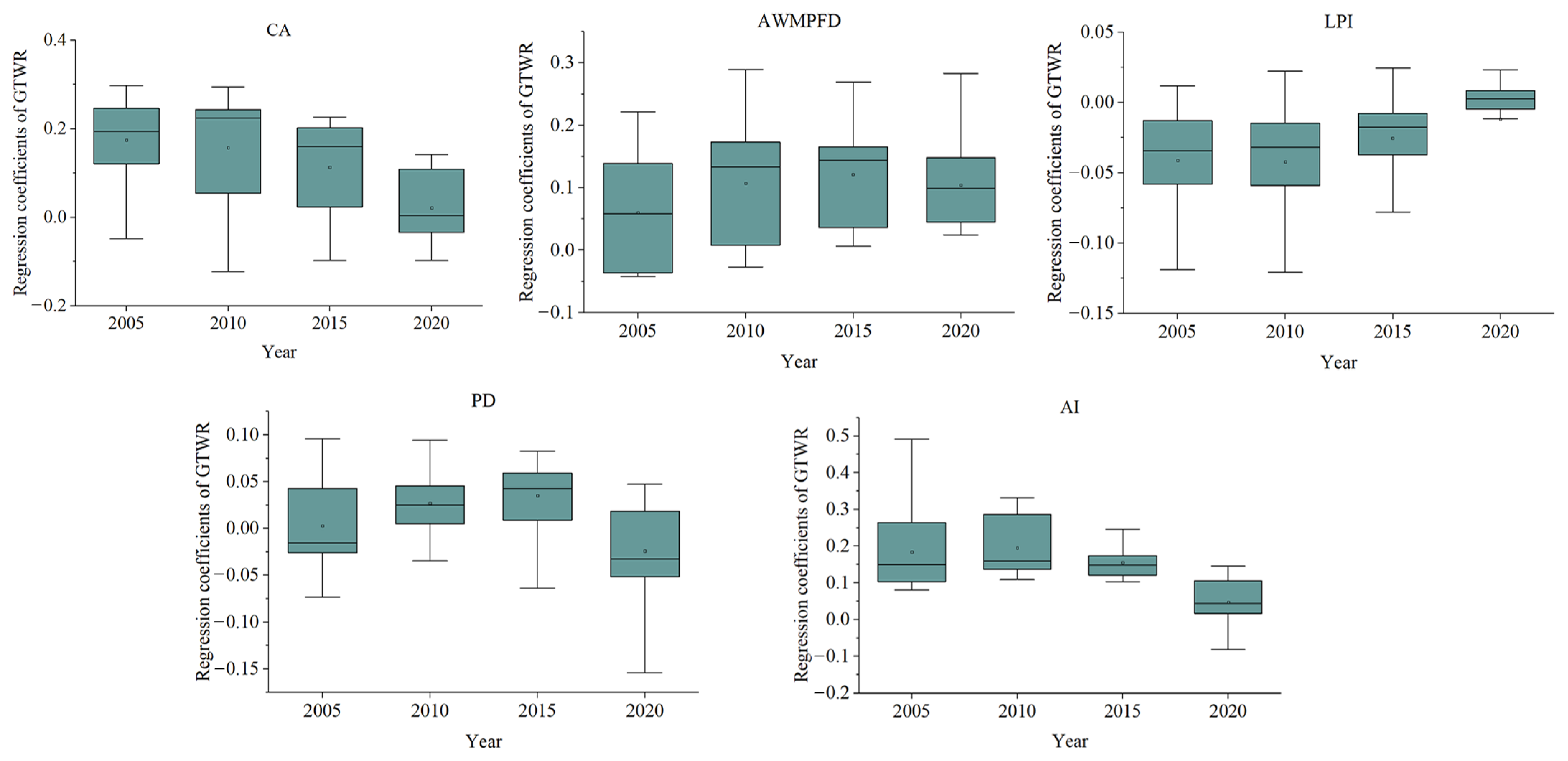
3.2. Temporal Characteristics of Association of USFIs and UERIs

We selected five landscape pattern metrics as independent variables and UERIs as the dependent variable and conducted GTWR analyses for these variables. During the study period, CA, AWMPFD, PD, AI, and UERIs showed a significant positive correlation, indicating that urban scale expansion, complexity of Urban Spatial Forms, urban spatial agglomeration, and patch connectivity are all factors conducive to UERIs. In contrast, LPI exhibited a negative correlation with UERIs, suggesting that mono-core urban development is not conducive to improving UER (Figure 6).

3.3. Spatial Characteristics of Association of USFIs and UERIs

Figure 7 displays the spatial distribution of the regression coefficient of CA on UERIs. In 2005, the distribution generally exhibited high values in the north and south of the city cluster and low values in the middle, with high values concentrated in Wuhan, Changsha, and their neighboring cities. By 2010, the regression coefficient increased in the western part of the city cluster, specifically in the cities of Changde, Yueyang, and Jingzhou. In 2015, the distribution of the regression coefficient of CA on UER showed distinctive characteristics, with high values in the western part and low values in the eastern part of the city cluster. However, in 2020, the regression coefficient of USFIs decreased significantly, leading to an increase in the number of cities with a negative regression coefficient of USFIs, rising from 5 cities to 12 in 2015.

Figure 8 demonstrates that the regression coefficients of AWMPFD on UERIs exhibited a spatial distribution characteristic of being low in the south and high in the east of the city cluster during the study period. In 2005, there were 12 cities with negative regression coefficients, which accounted for 42.86% of the total. By 2010, the number of negative regression coefficients had decreased to 5. However, from 2015 to 2020, the effect of the perimeter of AWMPFD on UERIs continued to increase, and AWMPFD had a positive impact on UERIs in all cities.

Figure 9 depicts the spatial distribution of the regression coefficients between LPI and UERIs. In 2005, the spatial distribution of the regression coefficients displayed a gradual increase from the northeast to the southwest within the city cluster in the YRM. At that time, the number of cities with negative regression coefficients accounted for 89% of the total number of cities. However, in 2010 and 2015, the regression coefficients of LPI and UERIs decreased. By 2020, all regression coefficients had turned negative, with high negative values mainly concentrated in the northwestern part of the city cluster, including cities like Xiangyang, Yichang, and Jingmen.

From Figure 10, it is evident that in 2005, the regression coefficient of PD on UERIs for the city cluster in the YRM exhibited spatial characteristics with low values in the west and south and high values in the northeast. By 2010, cities with high regression coefficients were primarily located in the northeast of the cluster, including Wuhan and its five neighboring cities, and the regression coefficients continued to increase in 2015. In 2020, the high values of the regression coefficient were distributed in the northwestern part of the urban agglomeration, including cities like Changsha, Xiangtan, and Yueyang.

Figure 11 revealed that in 2005, the spatial distribution of the regression coefficients of AI on UERIs in the urban cluster in the YRM was characterized by high values in the north and low values in the west and east, with the highest value in Wuhan and its neighboring cities. By 2010, the regression coefficients had increased. However, in 2015 and 2020, the effects of AI on UERIs decreased, although both remained positive.

3.4. Driving Influence of USFIs on UERIs and Interaction Detection

The original numerical values of the five USFIs were discretized using the box-allocating method. The values of UERIs and the discretized variables were then imported into the Geodetector for factor detection. Figure 12 illustrates the driving influence of USFIs on UERIs, indicating that LPI and AI are the primary drivers of UERIs, followed by CA and AWMPFD, with PD playing a lesser role as a driver. During the study period, the q-values of PD and LPI increased, while the q-values of CA, AI, and AWMPFD decreased. AI had the most significant impact on UERIs in 2005 and 2015, while LPI had the greatest influence on UERIs in 2010 and 2020.

The interaction detector was employed to reveal the interaction effects between the driving factors, and the results are presented in

Table 8. Results of interaction test in 2005.

	CA	PD	LPI	AI	AWMPFD		CA	PD	LPI	AI	AWMPFD
CA	0.485318					CA
PD	0.716976	0.104895				PD	EN
LPI	0.768259	0.421767	0.116938			LPI	EN	EN
AI	0.876579	0.821225	0.980676	0.660866		AI	EB	EN	EN
AWMPFD	0.903908	0.775401	0.881986	0.915069	0.282449	AWMPFD	EN	EN	EN	EB

,

Table 9. Results of interaction test in 2010.

	CA	PD	LPI	AI	AWMPFD		CA	PD	LPI	AI	AWMPFD
CA	0.487257					CA
PD	0.999241	0.198028				PD	EN
LPI	0.974956	0.912886	0.595530			LPI	EB	EN
AI	0.931536	0.815547	0.958240	0.555079		AI	EB	EN	EB
AWMPFD	0.958770	0.986579	0.887452	0.938365	0.391599	AWMPFD	EN	EN	EB	EB

,

Table 10. Results of interaction test in 2015.

	CA	PD	LPI	AI	AWMPFD		CA	PD	LPI	AI	AWMPFD
CA	0.243481					CA
PD	0.733859	0.299211				PD	EN
LPI	0.658995	0.874502	0.358011			LPI	EN	EN
AI	0.856488	0.646417	0.898574	0.267219		AI	EN	EN	EN
AWMPFD	0.861408	0.847432	0.840688	0.834502	0.352398	AWMPFD	EN	EN	EN	EN

and

Table 11. Results of interaction test in 2020.

	CA	PD	LPI	AI	AWMPFD		CA	PD	LPI	AI	AWMPFD
CA	0.213662					CA
PD	0.707491	0.146397				PD	EN
LPI	0.892034	0.806755	0.419132			LPI	EN	EN
AI	0.996662	0.999521	0.941814	0.351528		AI	EN	EN	EN
AWMPFD	0.841099	0.963180	0.988388	0.952343	0.227108	AWMPFD	EN	EN	EN	EN

. The results of the interaction detection can be categorized into two types: augmented and non-linear (EN, q($X1\cap X2$) > q(X1) + q(X2)), and augmented and bivariate (EB, q(X1) + q(X2) > q($X1\cap X2$) > MAX(q(X1), q(X2)). These findings suggest that during the research period, the impact of all interaction factors on the spatial heterogeneity of UERIs was significantly amplified compared to the individual influence factors. In 2005, 2010, 2015, and 2020, there were 6, 10, 7, and 9 key interaction factors, respectively, with 80% explanatory power of UERIs. This indicates that the two-factor effect on UERIs is significant, and there is a strong factor correlation between these factors. Among them, the key interaction factors with a high influence on UERIs include CA ∩ AI, CA ∩ AWMPFD, LPI ∩ AI, LPI ∩ AWMPFD, and AI ∩ AWMPFD.

4. Discussion

4.1. Adaptation of the DPSIR Framework to UER

The concept of resilience has evolved from engineering resilience to evolutionary resilience. In contemporary discussions, there is greater emphasis on adaptive capacity in complex situations rather than aiming for a stable ideal state. Evolutionary UER theory suggests that urban ecosystems, when subjected to external shocks or disturbances, undergo a process of stabilization, oscillation, and eventually reach a new stable state.

The DPSIR framework was initially employed to analyze the relationship between human activities and environmental changes. However, existing UER analyses often decompose the urban ecosystem into the resilience of economic, social, and natural subsystems, paying little attention to the positive or negative feedback between these subsystems. The causal logic of the DPSIR framework addresses these shortcomings and provides a more comprehensive evaluation method.

In our study, we enhanced the general DPSIR framework structure (Figure 13), originally proposed by the European Environment Agency (EEA), to reinforce the understanding of the process chain in our conceptual model [45]. The five types of indicators in our model thoroughly capture changes in UER, highlighting the socio-economic ‘driving’ forces that exert ‘pressure’ on urban ecological security, resulting in ‘state’ changes in urban ecology, resources, environment, and land use. These changes, in turn, impact ‘influence’ on human activities, ultimately leading to a series of ‘response’ initiatives that complete a causal chain (Figure 14). This approach enhances our research framework and ideas for the study of UER.

4.2. Responsiveness of USFIs on UER

Regarding the influencing factors of UER, most of the existing research considered the social ‘soft environment’ such as population [46], economy [19,20], science and technology [18], and urbanization [17], or the spatial ’hard environment’ such as land use, land development intensity [46], and infrastructure construction [21], but the influence of USF on UER has not been addressed. USF has proven to have a significant impact on urban carbon emissions [26,27], heat island effect [29], and other urban ecological effects, so we chose to focus on the influence of USF on UER. In this research, five landscape pattern indices (CA, AWMPFD, LPI, PD, AI) were selected to describe USF and analyze its impact on UER.

CA represents city size, and it exhibited a positive correlation with UER in 2005, 2010, 2015, and 2020. However, the strength of this positive correlation gradually weakened over time, with the percentage of cities showing a negative correlation in 2020 reaching 42.86%. This shift indicated that the promoting effect of city size expansion on ecological resilience diminished, and it began to exhibit inhibitory effects. Although urban scale expansion is often considered the primary cause of urban ecosystem degradation [47,48], the results of this study demonstrated that during the research period, urban scale expansion in the city cluster in the midstream of the Yangtze River had a positive impact on ecological resilience. This can be attributed to the fact that in the process of urbanization, the construction of new districts placed a greater emphasis on ecological environmental protection and the improvement of human habitat. Measures like increasing urban green spaces were taken to enhance the ecological resilience of the cities. Additionally, a significant number of rural populations migrated to the cities, leading to changes in local production and living styles, which reduced the pressure on ecosystem resources in the region. The negative impact of urban expansion on ecological resilience became more pronounced in 2020, aligning with the results of studies by other researchers. These studies have shown that urban expansion can lead to increased urban temperatures and concentrations of PM2.5, ultimately reducing the city’s ability to withstand risks.

AWMPFD characterizes the complexity of urban shape, and it is significantly and positively correlated with UER. The irregularity of urban shape is often associated with the non-uniform distribution of various functional zones within the city. In the context of urban planning in the YRM, there has been a substantial influx of population and capital. This influx has led to the development of new transport infrastructures and industrial parks, which have expanded urban boundaries, diversified urban fringe forms, and enhanced ecological safety within the city. These developments have been achieved through the integration of abandoned land, the addition of new green spaces, and the expansion of the transport network.

LPI, which describes the extent to which cities exhibit a monocentric development pattern, stands out as one of the primary drivers of spatial differentiation in UER. LPI shows a negative correlation with ecological resilience. This correlation highlights the potential risks associated with high levels of population and economic concentration in monocentrically developed urban areas, as well as the challenges of adapting urban disaster-resistant and emergency response resources to potential risks. In the event of natural disasters and ecological threats, monocentric cities may face greater difficulties in evacuating and providing essential aid to their residents. On the contrary, multi-center development can facilitate the balanced allocation of urban public facilities, resources, and services. This dispersion and diversification of resources can effectively mitigate risks and enhance UER.

PD characterizes the degree of urban agglomeration, and it exhibits a significant positive correlation with ecological resilience. This correlation suggests that the clustering of urban patches within the urban agglomeration in the YRM promotes ecological resilience. More compact cities have the advantage of enabling industries to generate cluster effects, which, in turn, lead to reduced transport and storage costs, as well as a decrease in environmental pollution.

AI describes urban connectivity, which is one of the main drivers of spatial heterogeneity in UER. AI shows a positive correlation with ecological resilience, signifying that increased connectivity in cities contributes to more sustainable development. Intra-city connectivity primarily manifests in the realm of commuting. Enhancing connectivity is beneficial for the development of public transport, leading to improved travel efficiency and reduced environmental pollution resulting from traffic and commuting.

4.3. Policy Suggestions and Prospects

• Ecological policies should extend beyond the urban scale. Urban development patterns should be chosen based on a comprehensive understanding of how urbanization impacts the urban scale and the factors driving structural security and ecosystem resilience. This includes the development of multi-center cities when feasible, where the central urban area plays a leading role in radiating influence. As urbanization progresses to a higher stage, a multi-center development model suitable for the city’s overall layout should be adopted. Effective planning should optimize the functions within the city center and facilitate communication between different city centers to ensure orderly city development.
• To enhance the construction of new districts in the urbanization process, strict adherence to ecological norms for green areas and building layouts is essential. This approach will significantly improve the ecological resilience of new districts.
• Promoting a concentrated and continuous urban structure is crucial. This can be achieved by enhancing intra-city transport and other infrastructure to reduce travel costs.

In future research, it is important to expand data collection channels, enhance data accuracy, and select more representative indicators for calculating UER. Additionally, there is a need to investigate the ecological resilience of different functional areas within cities, such as new and old cities, industrial and residential areas, and others, to better understand the mechanisms behind the spatial heterogeneity of ecological resilience.

5. Conclusions

In order to address sudden natural disaster events and formulate urban ecological strategies, the impact of USF on UER has gradually received attention. However, studies quantifying the impact of urban form on ecological resilience are still relatively scarce. Therefore, we quantified the spatiotemporal relationship between USF and UER in the YRM using the GTWR model and analyzed the drivers of UERIs using the geographical detector. Our conclusions are as follows:

• The level of ecological resilience in cities in the YRM significantly and continuously increased during study period. It exhibited a spatial distribution pattern with high values in the southeast, followed by the northwest, and low values in the central region. From 2005 to 2020, areas with “low–low” were primarily found in Wuhan and its surrounding cities.
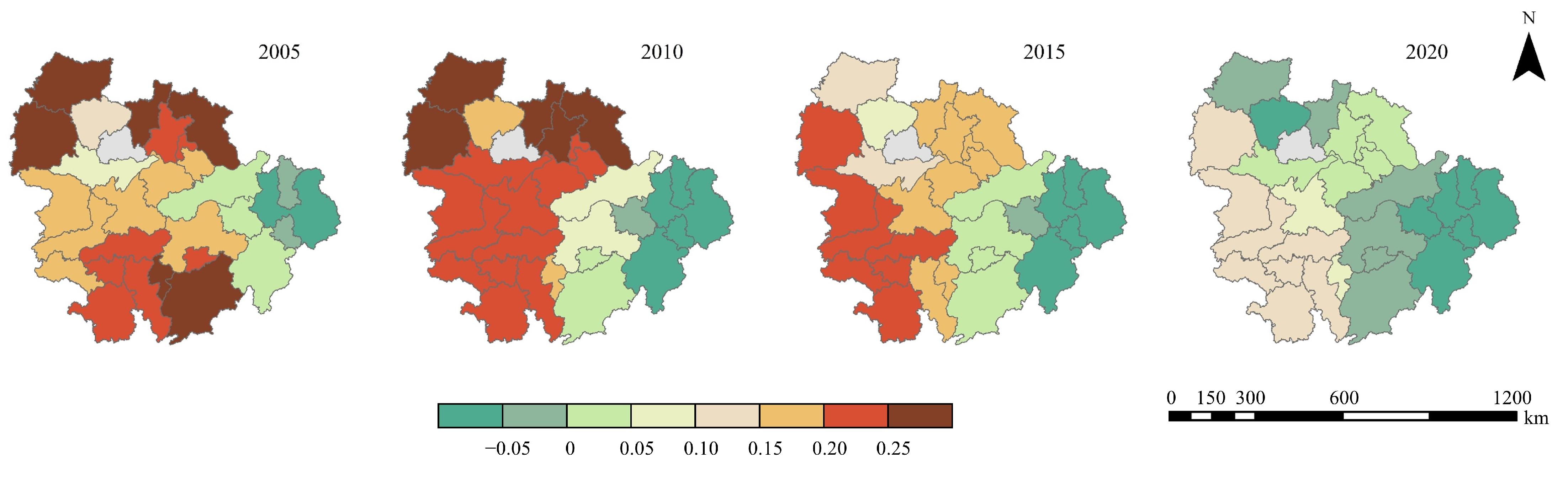
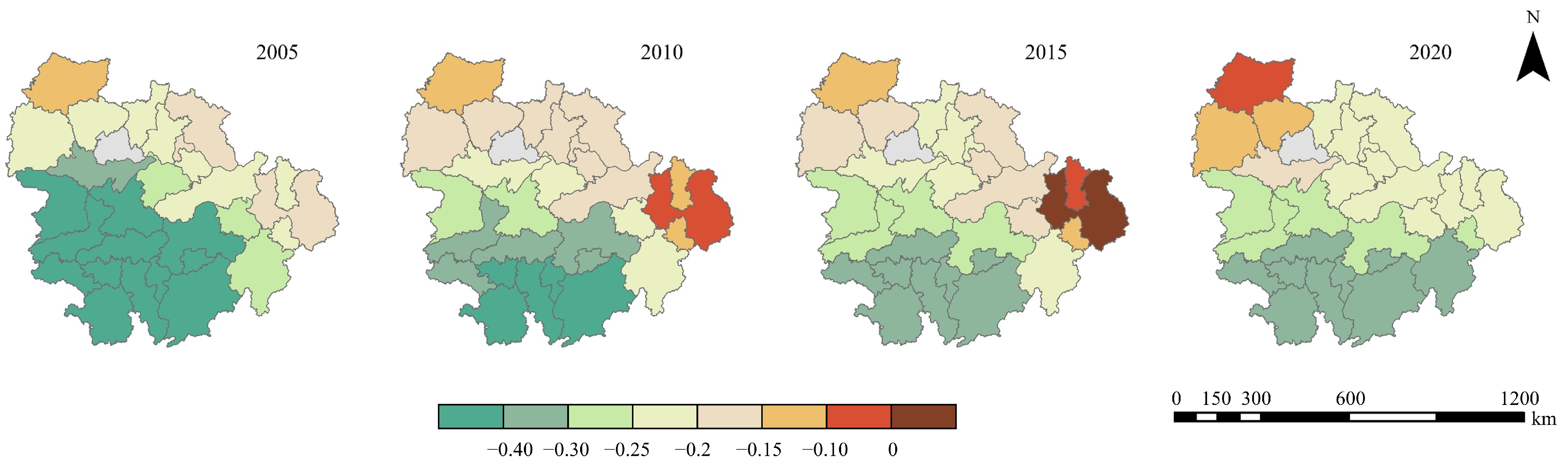
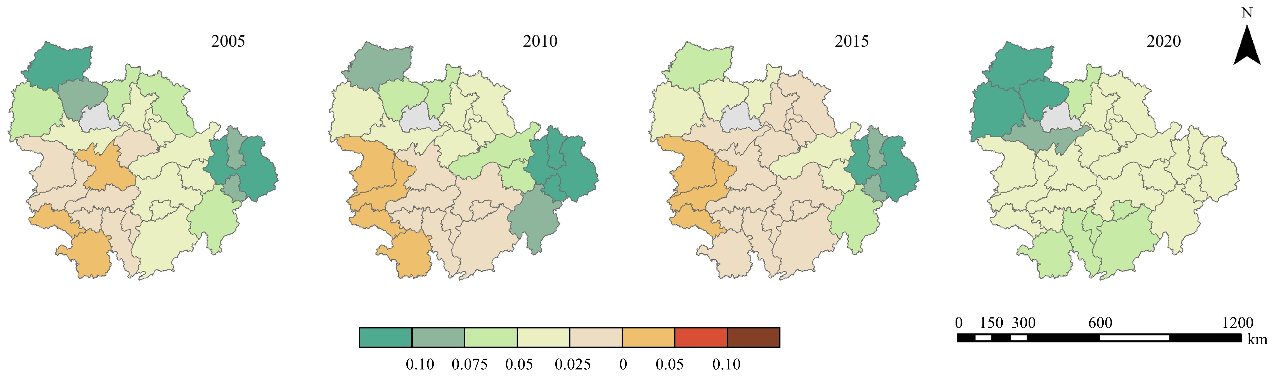
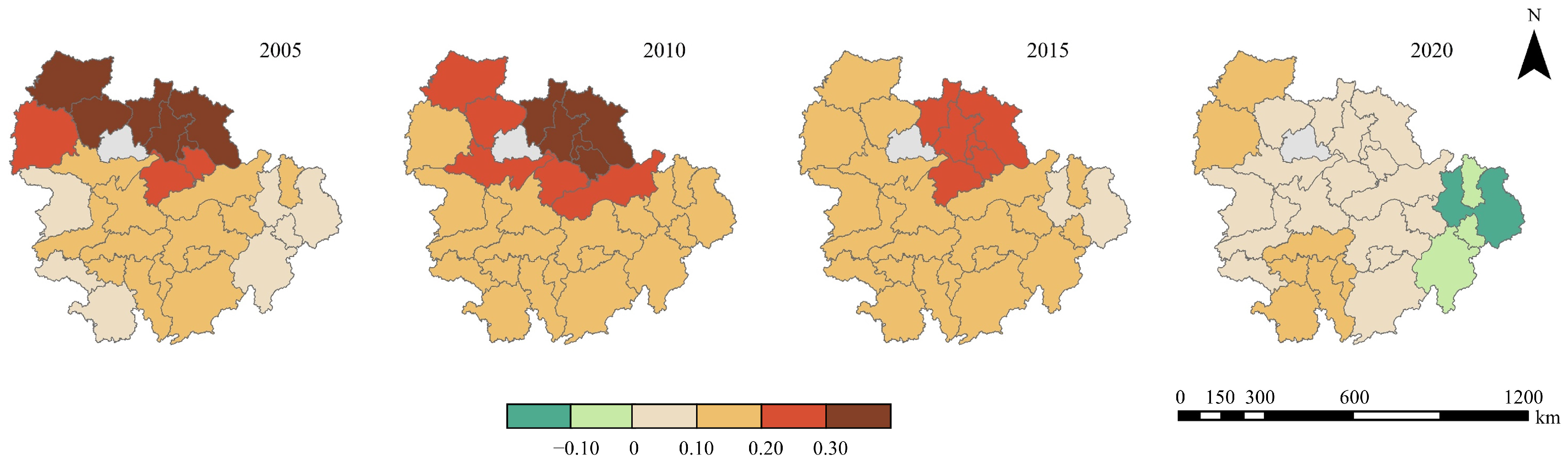
• A significant spatial and temporal relationship existed between USFIs and UERIs in the YRM in 2005, 2010, 2015, and 2020. The regression coefficients of USFIs and UERIs showed pronounced spatial and temporal variations. In the YRM, the mean values of the regression coefficients of CA on UERI decreased during each of the five years. The mean values of the regression coefficients for AWMPFD and AI on UERI gradually increased from 2005–2015 and decreased in 2020. The median values of the regression coefficients of LPI on UERI increased each five years. The mean values of the regression coefficients of PD on UERI increased in 2005–2015 but decreased to negative in 2020.
• CA, AWMPFD, PD, and AI had positive correlations with UERIs, indicating that urban scale expansion, complexity of urban spatial form, urban spatial agglomeration, and patch connectivity are all factors conducive to UERIs. In contrast, LPI exhibited a negative correlation with UERIs, suggesting that mono-core urban development is not conducive to improving UER.
• LPI and AI were the main drivers of spatial heterogeneity in UERIs, followed by CA and AWMPFD, with PD playing a lesser role as a driver. The interaction of these two factors significantly enhanced their influence on UERIs compared to their individual effects. Among them, the key interaction factors with a high influence on UERIs include CA ∩ AI, CA ∩ AWMPFD, LPI ∩ AI, LPI ∩ AWMPFD, and AI ∩ AWMPFD.

In future UER construction, we recommend the formulation of ecological policies that extend beyond the city scale. Urban development patterns should be chosen based on a comprehensive understanding of how urbanization affects city scale and the drivers of ecosystem structural security and resilience. Developing multi-center cities and improving the planning of new districts, urban agglomeration, and connectivity should be prioritized.

References

1. Sharifi, A. Co-benefits and synergies between urban climate change mitigation and adaptation measures: A literature review. Sci. Total Environ. 2021, 750, 141642. [Google Scholar] [CrossRef] [PubMed]
2. Nazmfar, H.; Saredeh, A.; Eshgi, A.; Feizizadeh, B. Vulnerability evaluation of urban buildings to various earthquake intensities: A case study of the municipal zone 9 of Tehran. Hum. Ecol. Risk Assess. Int. J. 2019, 25, 455–474. [Google Scholar] [CrossRef]
3. Mishra, S.V.; Gayen, A.; Haque, S.M. COVID-19 and urban vulnerability in India. Habitat Int. 2020, 103, 102230. [Google Scholar] [CrossRef]
4. Zandalinas, S.I.; Fritschi, F.B.; Mittler, R. Global warming, climate change, and environmental pollution: Recipe for a multifactorial stress combination disaster. Trends Plant Sci. 2021, 26, 588–599. [Google Scholar] [CrossRef] [PubMed]
5. Liang, L.; Wang, Z.; Li, J. The effect of urbanization on environmental pollution in rapidly developing urban agglomerations. J. Clean. Prod. 2019, 237, 117649. [Google Scholar] [CrossRef]
6. Masnavi, M.; Gharai, F.; Hajibandeh, M. Exploring urban resilience thinking for its application in urban planning: A review of literature. Int. J. Environ. Sci. Technol. 2019, 16, 567–582. [Google Scholar] [CrossRef]
7. Tong, Y.; Lei, J.; Zhang, S.; Zhang, X.; Rong, T.; Fan, L.; Duan, Z. Analysis of the Spatial and Temporal Variability and Factors Influencing the Ecological Resilience in the Urban Agglomeration on the Northern Slope of Tianshan Mountain. Sustainability 2023, 15, 4828. [Google Scholar] [CrossRef]
8. Wu, C.; Cenci, J.; Wang, W.; Zhang, J. Resilient city: Characterization, challenges and outlooks. Buildings 2022, 12, 516. [Google Scholar] [CrossRef]
9. Holling, C.S. Engineering resilience versus ecological resilience. Eng. Ecol. Constraints 1996, 31, 32. [Google Scholar]
10. Holling, C.S. Understanding the complexity of economic, ecological, and social systems. Ecosystems 2001, 4, 390–405. [Google Scholar] [CrossRef]
11. Liao, Z.; Zhang, L. Spatio-temporal analysis and simulation of urban ecological resilience in Guangzhou City based on the FLUS model. Sci. Rep. 2023, 13, 7400. [Google Scholar] [CrossRef] [PubMed]
12. Hammond, A.L.; World Resources Institute. Environmental Indicators: A Systematic Approach to Measuring and Reporting on Environmental Policy Performance in the Context of Sustainable Development; World Resources Institute: Washington, DC, USA, 1995; Volume 36. [Google Scholar]
13. Opschoor, H.; Reijnders, L. Towards sustainable development indicators. In Search of Indicators of Sustainable Development; Springer: Berlin/Heidelberg, Germany, 1991; pp. 7–27. [Google Scholar]
14. Segnestam, L. Indicators of Environment and Sustainable Development: Theories and Practical Experience; Number 89; World Bank: Washington, DC, USA, 2003. [Google Scholar]
15. Corvalan, C.; Nurminen, M.; Pastides, H. Linkage Methods for Environment and Health Analysis: Technical Guidelines; Office of Global and Integrated Environmental Health, WHO: Geneva, Switzerland, 1997. [Google Scholar]
16. Lyu, T.H.U.; Han, F.S.K.A. Spatial-temporal Analysis and Influencing Factors of Ecological Resilience in Yangtze River Delta. Areal Res. Dev. 2023, 42, 54–60. [Google Scholar]
17. Wang, S.; Cui, Z.; Lin, J.; Xie, J.; Su, K. The coupling relationship between urbanization and ecological resilience in the Pearl River Delta. J. Geogr. Sci. 2022, 32, 44–64. [Google Scholar] [CrossRef]
18. Zhou, Q.; Zhu, M.; Qiao, Y.; Zhang, X.; Chen, J. Achieving resilience through smart cities? Evidence from China. Habitat Int. 2021, 111, 102348. [Google Scholar] [CrossRef]
19. Hu, Y.; Zhang, Y.; Ke, X. Dynamics of tradeoffs between economic benefits and ecosystem services due to urban expansion. Sustainability 2018, 10, 2306. [Google Scholar] [CrossRef]
20. Zhao, K.; Xu, T.; Zhang, A. Urban land expansion, economies of scale and quality of economic growth. J. Nat. Resour. 2016, 31, 390–401. [Google Scholar]
21. Naess, P. Urban structures and travel behaviour: Experiences from empirical research in Norway and Denmark. Eur. J. Transp. Infrastruct. Res. 2003, 3, 153. [Google Scholar]
22. Simma, A.; Vrtic, M.; Axhausen, K.W. Interactions of travel behaviour, accessibility and personal characteristics: The case of the Upper Austria Region. In Proceedings of the European Transport Conference, Cambridge, UK, 10–12 September 2001; pp. 10–12. [Google Scholar]
23. Lv, B.; Sun, T. Study on spatial form compactness from low-carbon perspective. Geogr. Res. 2013, 32, 1057–1067. [Google Scholar]
24. Stern, N. A Blueprint for a Safer Planet: How to Manage Climate Change and Create a New Era of Progress and Prosperity; Random House: New York, NY, USA, 2009. [Google Scholar]
25. Jia, Y.; Tang, L. Environmental effects of the urban spatial form of Chinese cities. Acta Ecol. Sin 2019, 39, 2986–2994. [Google Scholar]
26. Yuan, Q.; Guo, R.; Leng, H.; Song, S. Research on the impact of urban form of small and medium-sized cities on carbon emission efficiency in the Yangtze River Delta. J. Hum. Settl. West China 2021, 36, 8–15. [Google Scholar]
27. Falahatkar, S.; Rezaei, F. Towards low carbon cities: Spatio-temporal dynamics of urban form and carbon dioxide emissions. Remote Sens. Appl. Soc. Environ. 2020, 18, 100317. [Google Scholar]
28. Fei, T.; Yanjun, W.; Mengjie, W.; Shaochun, L.; Yunhao, L.; Hengfan, C. Spatiotemporal coupling relationship between urban spatial morphology and carbon budget in Yangtze River Delta urban agglomeration. Acta Ecol. Sin 2022, 23, 9636–9650. [Google Scholar]
29. Liu, H.; Huang, B.; Zhan, Q.; Gao, S.; Li, R.; Fan, Z. The influence of urban form on surface urban heat island and its planning implications: Evidence from 1288 urban clusters in China. Sustain. Cities Soc. 2021, 71, 102987. [Google Scholar] [CrossRef]
30. China News. The Urbanisation Rate of China’s Resident Population Exceeded 65%, and Urbanisation Entered the “Second Half”. 2023. Available online: https://news.cctv.com/2023/03/29/ARTI0oMQJO0p8MNxpyBMCn3O230329.shtml (accessed on 5 October 2023).
31. Bai, Y.; Deng, X.; Jiang, S.; Zhang, Q.; Wang, Z. Exploring the relationship between urbanization and urban eco-efficiency: Evidence from prefecture-level cities in China. J. Clean. Prod. 2018, 195, 1487–1496. [Google Scholar] [CrossRef]
32. Hubacek, K.; Guan, D.; Barrett, J.; Wiedmann, T. Environmental implications of urbanization and lifestyle change in China: Ecological and water footprints. J. Clean. Prod. 2009, 17, 1241–1248. [Google Scholar] [CrossRef]
33. Xinhua News Agency. Opinions of the State Council on Accelerating the Construction of Ecological Civilisation. 2015. Available online: https://www.audit.gov.cn/n4/n18/c65045/content.html (accessed on 5 October 2023).
34. Xinhua News Agency. Outline of the Fourteenth Five-Year Plan for the National Economic and Social Development of the People’s Republic of China and the Vision 2035. 2021. Available online: https://www.gov.cn/xinwen/2021-03/13/content_5592681.htm (accessed on 5 October 2023).
35. Yanjie, X. Report on the Development of City Clusters in the Yangtze River Economic Belt (2019–2020); UNESCO Literature Publishing House: Paris, France, 2021. [Google Scholar]
36. He, P.; Zhang, H. Study on factor analysis and selection of common landscape metrics. For. Res. 2009, 22, 470–474. [Google Scholar]
37. Rezaee, F.; Jafari, M. Dynamic capability in an under-researched cultural environment. Manag. Sci. Lett. 2016, 6, 177–192. [Google Scholar] [CrossRef]
38. Chen, N.; Cheng, G.; Yang, J.; Ding, H.; He, S. Evaluation of Urban Ecological Environment Quality Based on Improved RSEI and Driving Factors Analysis. Sustainability 2023, 15, 8464. [Google Scholar] [CrossRef]
39. Zhao, R.; Fang, C.; Liu, H.; Liu, X. Evaluating urban ecosystem resilience using the DPSIR framework and the ENA model: A case study of 35 cities in China. Sustain. Cities Soc. 2021, 72, 102997. [Google Scholar] [CrossRef]
40. Lu, W.; Xu, C.; Wu, J.; Cheng, S. Ecological effect assessment based on the DPSIR model of a polluted urban river during restoration: A case study of the Nanfei River, China. Ecol. Indic. 2019, 96, 146–152. [Google Scholar] [CrossRef]
41. Han, B.; Liu, H.; Wang, R. Urban ecological security assessment for cities in the Beijing–Tianjin–Hebei metropolitan region based on fuzzy and entropy methods. Ecol. Model. 2015, 318, 217–225. [Google Scholar] [CrossRef]
42. Yin, L.; Zheng, W.; Shi, H.; Wang, Y.; Ding, D. Spatiotemporal Heterogeneity of Coastal Wetland Ecosystem Services in the Yellow River Delta and Their Response to Multiple Drivers. Remote Sens. 2023, 15, 1866. [Google Scholar] [CrossRef]
43. Wei, H.; Han, Q.; Yang, Y.; Li, L.; Liu, M. Spatial Heterogeneity of Watershed Ecosystem Health and Identification of Its Influencing Factors in a Mountain–Hill–Plain Region, Henan Province, China. Remote Sens. 2023, 15, 3751. [Google Scholar] [CrossRef]
44. Zhang, S.; Wang, Y.; Xu, W.; Sheng, Z.; Zhu, Z.; Hou, Y. Analysis of Spatial and Temporal Variability of Ecosystem Service Values and Their Spatial Correlation in Xinjiang, China. Remote Sens. 2023, 15, 4861. [Google Scholar] [CrossRef]
45. Smeets, E.; Weterings, R. Environmental Indicators: Typology and Overview; Technology and Policy: Amsterdam, The Netherlands, 1999. [Google Scholar]
46. Zhan, M.; Ren, Y. Spatiotemporal evolution characteristics and influencing factors of urban ecological resilience in the Yellow River Basin. Arid. Land Geogr. 2023, 7, 335. [Google Scholar]
47. Uttara, S.; Bhuvandas, N.; Aggarwal, V. Impacts of urbanization on environment. Int. J. Res. Eng. Appl. Sci. 2012, 2, 1637–1645. [Google Scholar]
48. Seto, K.C.; Sánchez-Rodríguez, R.; Fragkias, M. The new geography of contemporary urbanization and the environment. Annu. Rev. Environ. Resour. 2010, 35, 167–194. [Google Scholar] [CrossRef]
49. McGarigal, K.; Cushman, S.A.E.E. FRAGSTATS v4: Spatial Pattern Analysis Program for Categorical and Continuous Maps. 2015. Available online: https://www.researchgate.net/publication/255981347 (accessed on 11 October 2023).
Figure 1. Study area. (a): The location of the study area in China. Note: the base map of China (review number: GS (2020) 4623, http://bzdt.ch.mnr.gov.cn, accessed on 20 September 2023) was sourced from the standard map service system of the Ministry of Natural Resources, China, and the boundary of the base map has not been modified. (b): 28 prefecture-level cities in the study area.
Buildings 14 00274 g001
Figure 2. Spatial form and landscape metrics of three cities in the YRM.
Buildings 14 00274 g002
Figure 3. The UERIs comparison between 2005 and 2020.
Buildings 14 00274 g003
Figure 4. Spatial differentiation of UERIs in 2005, 2010, 2015, and 2020.
Buildings 14 00274 g004
Figure 5. Spatial autocorrelation analysis of UERIs in 2005, 2010, 2015, and 2020.
Buildings 14 00274 g005
Figure 6. The box diagram of GTWR regression coefficient of USFIs and UERIs in 2005, 2010, 2015, and 2020.
Buildings 14 00274 g006
Figure 7. The spatial distribution of the regression coefficient of CA on UERIs in 2005, 2010, 2015, and 2020.
Buildings 14 00274 g007
Figure 8. The spatial distribution of the regression coefficient of AWMPFD on UERIs in 2005, 2010, 2015, and 2020.
Buildings 14 00274 g008
Figure 9. The spatial distribution of the regression coefficient of LPI on UERIs in 2005, 2010, 2015, and 2020.
Buildings 14 00274 g009
Figure 10. The spatial distribution of the regression coefficient of PD on UERIs in 2005, 2010, 2015, and 2020.
Buildings 14 00274 g010
Figure 11. The spatial distribution of the regression coefficient of AI on UERIs in 2005, 2010, 2015, and 2020.
Buildings 14 00274 g011
Figure 12. Driving influence of USFIs on UERIs in 2005, 2010, 2015, and 2020.
Buildings 14 00274 g012
Figure 13. General DPSIR model (adapted from the literature [45]).
Buildings 14 00274 g013
Figure 14. Verbeterd DPSIR model.
Buildings 14 00274 g014