Article

Simulation of Water Flow Path Length (WFPL) and Water Film Depth (WFD) for Wide Expressway Asphalt Pavement

1
Guangdong Province Communications Planning & Design Institute Co., Ltd., Guangzhou 510641, China
2
School of Civil Engineering and Transportation, South China University of Technology, Guangzhou 510006, China
*
Author to whom correspondence should be addressed.
Buildings 2024, 14(1), 254; https://doi.org/10.3390/buildings14010254
Submission received: 4 December 2023 / Revised: 27 December 2023 / Accepted: 2 January 2024 / Published: 17 January 2024

Abstract

:
This paper simulates actual rainfall conditions and raindrops flowing to form a water flow path (WFP) on the pavement surface of the wide expressway. Then, the different linear combination conditions, including longitudinal slope (LS), transverse slope (superelevation, TS), gradual change rate of TS, and pavement width (PW), were simulated and analyzed. The results show that (1) the influence of each linear index on the maximum water film path length (WFPLmax) and maximum water flow depth (WFDmax) differs (according to the absolute values of Beta, LS has the greatest influence on WFPLmax, and PW has the greatest influence on the WFDmax for both straight-line and circular-curve sections); (2) when the design value of LS is between 1.1% and 4%, the WFDmax can be effectively reduced by lowering the value of LS; (3) in the case of a high design value of LS, it can be considered to increase the TS of the pavement arch from 2% to 2.5% to effectively reduce the WFPLmax, and the wider PW, the better the reducing effect; (4) while widening the expressway, adjusting the TS from 2% to 2.5% can effectively offset the increasing effect of PW on the WFDmax. This research aims to fill the research gap in the simulation of runoff characteristics of wide expressway asphalt pavements and to improve the alignment design of expressways from the drainage perspective for the improvement of driving safety.

1. Introduction

With the expansion of the expressway, the early two-way four lanes have gradually changed to two-way eight lanes or more. The increase in pavement width increases the water flow path length (WFPL) in rainy conditions, resulting in an increase in the water film depth (WFD) and the occurrence of hydroplaning, threatening driving safety [1,2,3]. The formation of water on expressway pavements depends entirely on the WFD, and the definition of the WFD of pavement needs to be clarified due to the differences in the texture depth. The WFD is defined as the sum of the WFD of the surface and the average texture depth [4,5]. Factors affecting the WFD include rainfall intensity, the WFPL, and the geometric linear index of the road [6,7]. Among them, the geometric characteristics of the pavement are determined by the plane line, longitudinal line, and cross-section, and the combination of plane and longitudinal line and cross-section are not completely independent, and their interaction also determines whether the geometric indexes meet the linear requirements. The WFP refers to the rainwater that falls on the pavement surface and begins to flow after a certain period. The water passes through the pavement surface along the synthetic slope direction under the action of gravity, generating a certain water film thickness [8,9]. The geometric characteristics of the pavement are the key factors determining the runoff behavior, which determines the WFP, including the runoff direction, the runoff velocity, and the length of the drainage path [10]. The geometry indexes related to the synthetic slope mainly include the longitudinal slope (LS), transverse slope (superelevation, TS), gradual change rate of TS, and geometry indicators related to the pavement surface, which is mainly pavement width (PW). The analysis of runoff characteristics should consider the influence of properties of the road itself, and the two-dimensional model of the pavement surface can describe the time-varying process of the runoff more completely compared with the one-dimensional model [11,12,13,14,15].

2. Literary Review

A series of results and findings have been achieved in the research on the simulation and calculation of asphalt pavement runoff path and the WFD. Luo et al. stated that the simulation and analysis of pavement runoff should be combined with the attribute characteristics of the pavement itself [16]. Zhang et al. analyzed the effect of road slope on the WFD and found that the effect of TS on WFD was greater than that of LS [17]. Richard et al. proposed formulae for calculating the WFDmax for straight lines, circular curves, and vertical curves [18]. Guo et al. obtained a prediction model of the runoff of road surface through simulation and calculation and analyzed the effects of rainfall intensity, LS, TS, and roadside drainage mode on the runoff [19]. Qi et al. used a combination of theoretical analysis, outdoor tests, and numerical simulation means to study runoff behavior under different alignment combinations at a certain rainfall condition. The linear combination threshold of a two-way six-lane road with a design speed of 120 km/h under rainy conditions was obtained, which does not affect driving safety [10].
Regarding the prediction model of the WFD on pavement surface under rainfall conditions, a series of studies have been carried out, and a variety of WFD prediction models have been established, mainly including regression models [16], mathematical–physical models [18], and neural network models [20]. Rainfall is the main water source of pavement runoff, and the existing models of the relationship between rainfall and runoff of the road surface can be divided into empirical models and hydrodynamic models [21,22]. Empirical models are easily restricted by testing conditions and cannot express the continuous time-varying characteristics of the flow field, while hydrodynamic models, including kinematic waves, power waves, and diffusion wave models, are widely applicable [23]. Cea et al. analyzed the WFD of the pavement surface in an urban area using a two-dimensional average depth prediction model and found that the two-dimensional model can better express the changes in the flow field [24]. Staufer et al. analyzed the changing characteristics of runoff under the influence of different factors and simulated the WFD of runoff by using a complete power wave [25]. Ma et al. predicted the WFD using an artificial neural network model, but their results were desirable when the input and output variables were within the range of the training samples [6]. Li et al. found that pavements go through the stages of wetting, flow production, steady state confluence, and receding in sequence for natural rainfall events, which is a nonlinear time-varying process on a two-dimensional space [26,27,28].
Currently, simulation and calculation studies of the WFPL and WFD are mostly based on two-way four/six-lane roads, and the applicability to wide expressways needs further investigation. In addition, measurements of WFD are based on indoor scale model experiments that are difficult to perform in the actual field. Therefore, in this paper, the DPM model in Fluent fluid simulation software is used to simulate the actual rainfall conditions, and the EWF model is applied to simulate the raindrops flowing on the road surface. Different linear combination conditions of wide expressway, including the LS, TS, gradual change rate of TS, and PW, were considered and simulated. The simulation results of the WFPL and WFD distribution, the WFPLmax, and the WFDmax of the straight-line section or circular-curve section are analyzed, and on this basis, the optimization suggestions of linear indexes for drainage requirements of wide expressways are proposed. This study aims to fill the research gap in the simulation of runoff characteristics of wide expressway pavements and to improve the alignment design of expressways from the drainage perspective. The novelty of this research lies in the extension of the simulation and calculation studies of WFPL and WFD to the wide expressway asphalt pavement, which has eight/ten/twelve-lane roads. In addition, the DPM model and the EWF model are applied to simulate actual rainfall conditions and the raindrops flowing on the road surface.
Next, Section 3 introduces the methodology with which to simulate the pavement runoff characteristics in rainy conditions and predict the WFD values of straight-line sections and circular-curve sections. Section 4 shows and discusses the simulation results of the distribution of WFPL and WFD and the WFPLmax of the straight-line section and the circular-curve sections under different linear combination conditions. Section 5 gives the conclusions of this paper based on the simulation results and analysis obtained from Section 4.

3. Methodology

To simulate the pavement runoff characteristics in rainy conditions, the Fluent software was selected, and the DPM model was applied. To predict the WFD values of straight-line sections and circular-curve sections of wide expressway pavement, a WFD prediction model was proposed, and the different linear combination conditions were selected.

3.1. Modelling of the Pavement

In this study, ANSYS Fluent 2022 was selected for the simulation of pavement runoff characteristics in rainy conditions. The used model in this study consists of a pavement triangular mesh surface model and a rainfall model. The pavement surface model consists of several triangular mesh planes with 1 m side length (see Figure 1), and the triangular mesh is generated by cutting the model generated from the HintCAD 8.0.5 version.
The formation of runoff on the pavement surface after rainfall is a complex two-phase interaction process which can be decomposed into two processes: the formation of raindrops and the falling; and the formation of runoff after contact with the pavement surface. The rainfall area was constructed in the form of a rectangle, with the top surface of the rectangle defined as the rainfall inlet plane (velocity inlet), and the rest of the surface defined as the water outlet (pressure outlet), as shown in Figure 2. The pavement model is located in the rainfall region (see the light blue area in Figure 3), which forms a whole with the rectangular body through shared topology. Raindrop particles are shot in from the top surface of the model and fall on the pavement surface to form a water film, which flows under gravity and surface tension and is removed from the pressure outlet.

3.2. Selection of Simulation Models

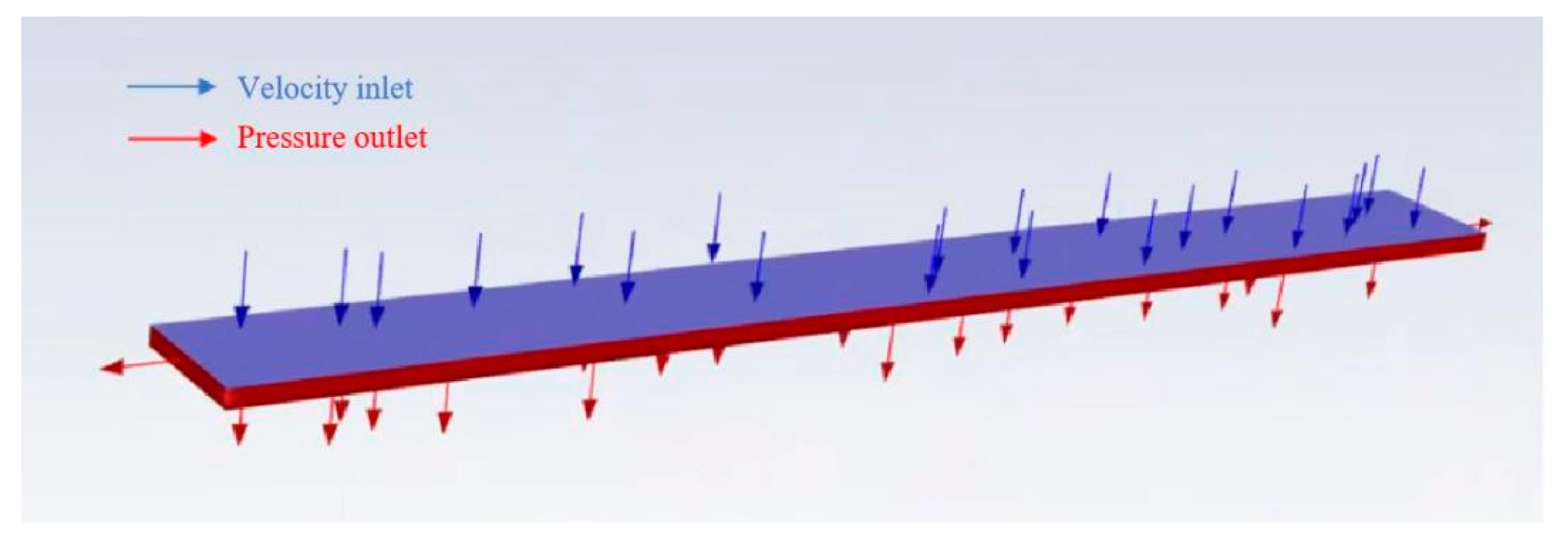
3.2.1. Rainfall Simulation

Rainfall simulation was performed through the simulation of raindrop particle injection with a certain rainfall intensity on the surface of a pavement geometry model. Conditions to be met include the following:
  • The flow input is stable and consistent with the set rainfall intensity;
  • The range of simulated rainfall needs to completely cover the surface of the pavement geometry model, and the spatial distribution is uniform and reasonable;
  • The flow inputs in the form of raindrops during rainfall should be reproduced in a granular manner as far as possible;
  • The duration of rainfall can be controlled to simulate rainfall within a certain time interval.

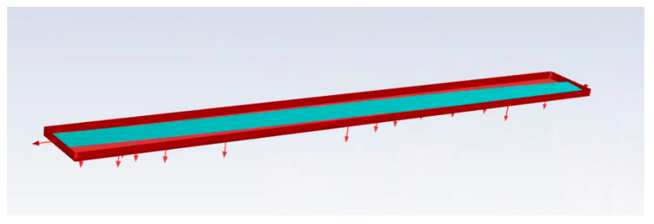
3.2.2. Runoff Simulation

Runoff simulation was conducted via simulation of the water flow on the pavement surface and the distribution of WFD in each area of the pavement, etc. Conditions to be met include the following:
  • Can be computed with the DPM model to collect DPM fluid particles and form a water film on the surface of the pavement geometry model;
  • Able to simulate the flow of runoff on the pavement surface, tracking the water film in the selected area under the action of gravity, surface tension, etc., to form runoff and flow out of the pavement width dissipation;
  • Can visualize the depth distribution of water on the pavement surface at different locations in the form of WFD.
Combining the above simulation needs, the DPM model was chosen to simulate rainfall, reflecting the raindrop size by the diameter of DPM particles and describing the intensity of rainfall by setting the second-phase flow rate. The EWF model was used to collect the DPM raindrop particles and realize the fluid flow on the surface of the pavement model, tracking the flow of the water film in the selected area after it had been aggregated into the runoff.

3.3. Rainfall Condition Simulation

The DPM model is a simulation of the rainfall process. Based on selecting flow as turbulence and discrete-phase particles as liquid water, raindrop particle diameter, rainfall start time and stop time, rainfall speed, and rainfall intensity need to be determined [29]. The diameter of raindrops is not constant during rainfall, and the average diameter of raindrops will change with the real-time change in rainfall intensity. In relevant studies, the average diameter of raindrops under different rainfall intensities is shown in Table 1.
In this study, the average diameter of raindrops was 2.86 mm via interpolation method according to the rainfall intensity of 60 min rainfall duration once in five years. Concerning the previous setting of the boundary, the rainfall duration of 60 min was selected to take the rainfall intensity as 0.0242 mm/s within 120 s after the start of rainfall (start time was 0 s and stop time was 120 s).

3.4. WFD Prediction Model

This paper analyzed and compared the regression formulae of the existing more-classical WFD prediction models, mainly including the model proposed by Luo, the model proposed by Ji, the Gallway model, the Wambold model, etc., to determine the parameters of the WFD prediction model of this paper and its experimental conditions, as follows:
(1)
The model proposed by Luo et al. [16]:
W D = 0.068 × L 0.32 · I 0.41 · T X D 1.17 S 0.31 .
(2)
The model proposed by Ji et al. [30]:
h = 0.1258 · l 0.6715 · i 0.3147 · r 0.7786 · T D 0.7261 .
(3)
The Gallaway model [31]:
d = 0.1664 · T 0.11 · L 0.43 · I 0.59 · S 0.42 T .
(4)
The Wambold model [32]:
d = 5.979 × 10 3 · T 0.11 · I 0.59 · S 0.42 T .
From these four models, it can be seen that the factors affecting the WFD in the regression models include the four parameters: rainfall intensity, road slope, WFPL, and textile depth. It can be seen from the WFD prediction model that rainfall intensity is the only environmental factor that affects the WFD considered in the above four models, which is one of the assumptions of the above model; i.e., it is assumed that rainfall intensity is a stable variable that does not change over time. The model structure of the WFD model in this study was similar to the above model, but the parameters need to be comprehensively determined based on the indoor and outdoor simulated rainfall tests and are assumed to be modeled as follows:
d = K · I k 1 · L k 2 · S k 3   · T k 4 ,
where d—WFD (mm); L—WFPL (m); S—road slope (%); I—rainfall intensity (mm/min); T—texture depth (mm); and K, k1, k2, k3, k4—regression coefficient.
A multivariate linear regression equation is obtained by transforming it logarithmically:
ln d = ln K + k 1 ln I + k 2 ln L + k 3 ln S + k 4 ln T .
After the multiple linear regression equations were analyzed, the regression equations and regression coefficients were tested for significance, where the F test was used for the regression equation and t testing was used for the significance of the regression coefficients.

3.5. Linear Combination Conditions

3.5.1. Straight-Line Section

In the simulation of the straight-line section, the right side of the straight-line section with 2% TS arch and without LS was first selected to verify the validity of the simulation. Then, the following linear combination conditions (Table 2), including the number of lanes per side, LS, and TS, were selected for simulation and analysis according to the current specification requirement [33].

3.5.2. Circular-Curve Section

In the circular-curve section, the inner and outer sides of the roadway reach the same TS. For the inner section of the left-deflected circular curve, the synthetic LS direction is pointing from the middle line to the shoulder, which is consistent with the synthetic slope situation of the arch in the straight section, and the WFDmax occurs on the shoulder side of the expressway. The water film of the inner lane is relatively small, and it will not affect driving safety. As for the outer section of the circular curve, the synthetic LS direction points from the shoulder to the median strip, and the endpoint of WFP is located in the left curb strip, which may lead to the high WFD value of the inner lane and affect driving safety. In addition, under the condition of a design speed of 120 km/h, whether the minimum TS of 2% for circular curves suggested by the specification applies to wide circular-curve sections needs to be examined and discussed. Based on the above reasons, the following linear combination conditions were selected for simulation analysis (Table 3).

4. Results and Discussion

According to the simulation, the results for the distribution of WFPL and WFD, as well as the WFPLmax of the straight-line section and the circular-curve sections under different linear combination conditions, were presented and analyzed, respectively. The results show that LS has the greatest influence on the WFPLmax, while PW has the greatest influence on the WFDmax.

4.1. Simulation Results and Discussion of Straight-Line Sections

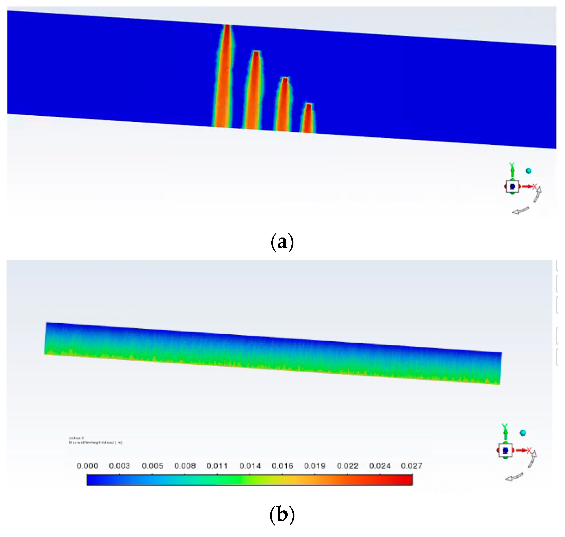
4.1.1. Distribution of the WFPL and WFD

For the straight-line section without the LS, the right side of the pavement with eight lanes in both directions and a 2% TS was selected to verify the validity of the simulation. The WFPL and WFD distribution simulation results are shown in Figure 4. It can be seen that the direction of runoff on the pavement surface is the same as that in the direction of TS (Figure 4a). With a WFPL of 18.75 m, the WFD shows an increasing trend from the inner side of the travel lanes to the outer side (Figure 4b). The simulation results are consistent with the actual situation, and the validity of the simulation was verified. Thus, the simulation can be considered effective.
For the straight-line section with LS, WFPL and WFD distribution maps were obtained from the simulation of a two-way eight-lane section with a section length of 300 m, LS of 0.5%, and TS of 2%. The WFPL and WFD distribution simulation results are shown in Figure 5, which shows that the WFP flow direction is the same as that of the synthetic LS direction, and the WFD shows an incremental tendency from the inner side of the traveled roadway to the outer side. The results of the above simulation lead to the preliminary conclusion that the WFP flows from the inside of the roadway to the outside of the straight roadway, and the WFD gradually increases as the WFP moves away from the center median.

4.1.2. Maximum Water Film Path Length (WFPLmax)

Under different LS and TS combinations, the WFPLmax of the straight-line sections of the two-way eight-lane, ten-lane, and twelve-lane road sections were simulated, and the results of all the linear combinations of conditions are shown in Table 4. When the PW and TS are the same, the WFPLmax values are positively correlated with LS. When the arch TS is 2%, the WFPL of 4% LS under two-way eight lanes is 2.23 times that of 2% LS. The WFPL of 4% LS under two-way ten lanes is 2.19 times that of 2% LS. The WFPL of 4% LS under two-way twelve lanes is 2.20 times that of 2% LS. Although the increase in LS allows for an increase in the synthetic slope, its direction is gradually biased in the direction of LS and leads to an increase in the WFPLmax. In addition, increasing the TS from 2% to 2.5% under the same LS condition effectively reduces the WFPLmax. This can be explained by the fact that the increase in TS increases the synthetic slope and, at the same time, makes the direction of the WFP gradually biased in the direction of TS, and since the transverse width of the pavement is much smaller than the longitudinal length, this makes the WFPL decrease, effectively reducing the WFPLmax. Furthermore, under a certain TS and LS, the greater the number of lanes, the longer the WFPLmax. This is because under a certain TS and LS, the direction of the WFP remains unchanged, while the increase in the number of lanes makes the PW increase. The WFPL becomes longer, so the WFPLmax also becomes longer accordingly.
The results of the WFPLmax reduction since the change of TS from 2% to 2.5% for different numbers of lanes at 120 km/h are shown in Table 5. For a certain number of lanes, the larger the LS, the more significant the reduction of the WFPLmax when the TS is changed from 2% to 2.5%. For a two-way eight-lane pavement, changing TS from 2% to 2.5%, the reduction of WFPLmax at 4% LS is 5.50 m, which is 78 times the decrease corresponding to 0.3% LS (0.07 m). For the two-way ten-lane pavement, changing TS from 2% to 2.5%, the reduction of WFPLmax at 4% LS is 6.81 m, which is 85 times the decrease in the corresponding 0.3% LS. For the two-way twelve-lane pavement, the reduction of WFPLmax at 4% LS is 90 times the decrease corresponding to 0.3% LS. Moreover, the reduction of WFPLmax by changing TS from 2% to 2.5% is not only obvious with the increase in LS but also significant with the increase in PW. It can be seen that in the case of limited-alignment and large-design LS, it can be considered to increase the TS of the pavement arch from 2% to 2.5% to effectively reduce the WFPLmax, and the wider the PW, the better the improvement effect.
Considering that in the above analysis, there is mutual influence among the TS, LS, and PW indicators, it is not possible to accurately rank the influence degree of each indicator on the WFPLmax; therefore, a linear regression analysis was carried out by using SPSS to compare using the standardized coefficient absolute value, and the results of the analysis are shown in Table 6. As can be seen from Table 6, when using the absolute value of the standard coefficient for comparison, LS has the greatest influence on WFPLmax, followed by PW, and TS has the least influence.

4.1.3. Maximum Water Flow Depth (WFDmax)

The results of the WFDmax, WFD on the first lane middle line, and WFD on the second lane middle line of the straight-line sections under different LS, TS, and PW conditions at 120 km/h are shown in Table 7 and Table 8. For the 120 km/h design speed, the WFDmax and WFD values on the first/second lane middle line are not greater than 5.03 mm, being lower than the safe WFD thresholds and meeting the needs of traffic safety. When PW is the same and the TS is fixed at 2% or 2.5%, the WFDmax and WFD values are positively correlated with LS; i.e., the increase in LS makes the WFD generally increase. This is because when the TS is the same, the increase in LS makes the synthetic slope direction biased towards the longitudinal direction of the pavement, the WFPLmax becomes longer, and the retention time of the surface water in the pavement becomes longer, which increases the WFD.
Moreover, when the LS is the same, increasing the TS from 2% to 2.5% can effectively reduce the WFD. As the LS and PW increase, increasing the TS is more effective in the WFD. This not only increases the synthetic slope of the pavement and accelerates the drainage process but also gradually biases the direction of the WFP in the direction of the TS, which shortens the WFPL because the transversal width of the pavement is much smaller than the longitudinal length, which reduces the WFPL, and the retention time in the pavement surface is shortened, so the WFD is greatly reduced.
The relationship between the change rate of the WFDmax and the LS is shown in Figure 6, and it can be seen that the WFDmax keeps increasing with the increase in LS. The trend of the WFDmax change with LS under different PW conditions is relatively close; i.e., the change rate shows a process of slow to fast and then to slow. In the case of LS less than 2.2%, the increase rate of the WFDmax becomes faster as LS increases. For LS greater than or equal to 2.2%, the WFDmax change rate becomes slower with the increase in LS. Therefore, when LS is between 1.1% and 4%, the change in LS has a greater effect on the change rate of the WFDmax than when LS is between 0.3% and 1.1%. It can be concluded that the WFDmax can be effectively reduced by decreasing the LS when LS is between 1.1–4%, and it is not recommended to prioritize the adjustment of LS to reduce the WFDmax when the LS is less than 1.1%.
The following linear regression analysis was carried out using SPSS to rank the effect degree of the TS, LS, and PW on the WFDmax regarding the absolute value of the standardized coefficient, and the results of the analysis are shown in Table 9. As can be seen from Table 9, when using the absolute value of the standard coefficient for comparison, the PW has the greatest impact on the WFDmax, followed by the TS, and the LS has the least impact.

4.2. Simulation Results and Discussion of Circular-Curve Sections

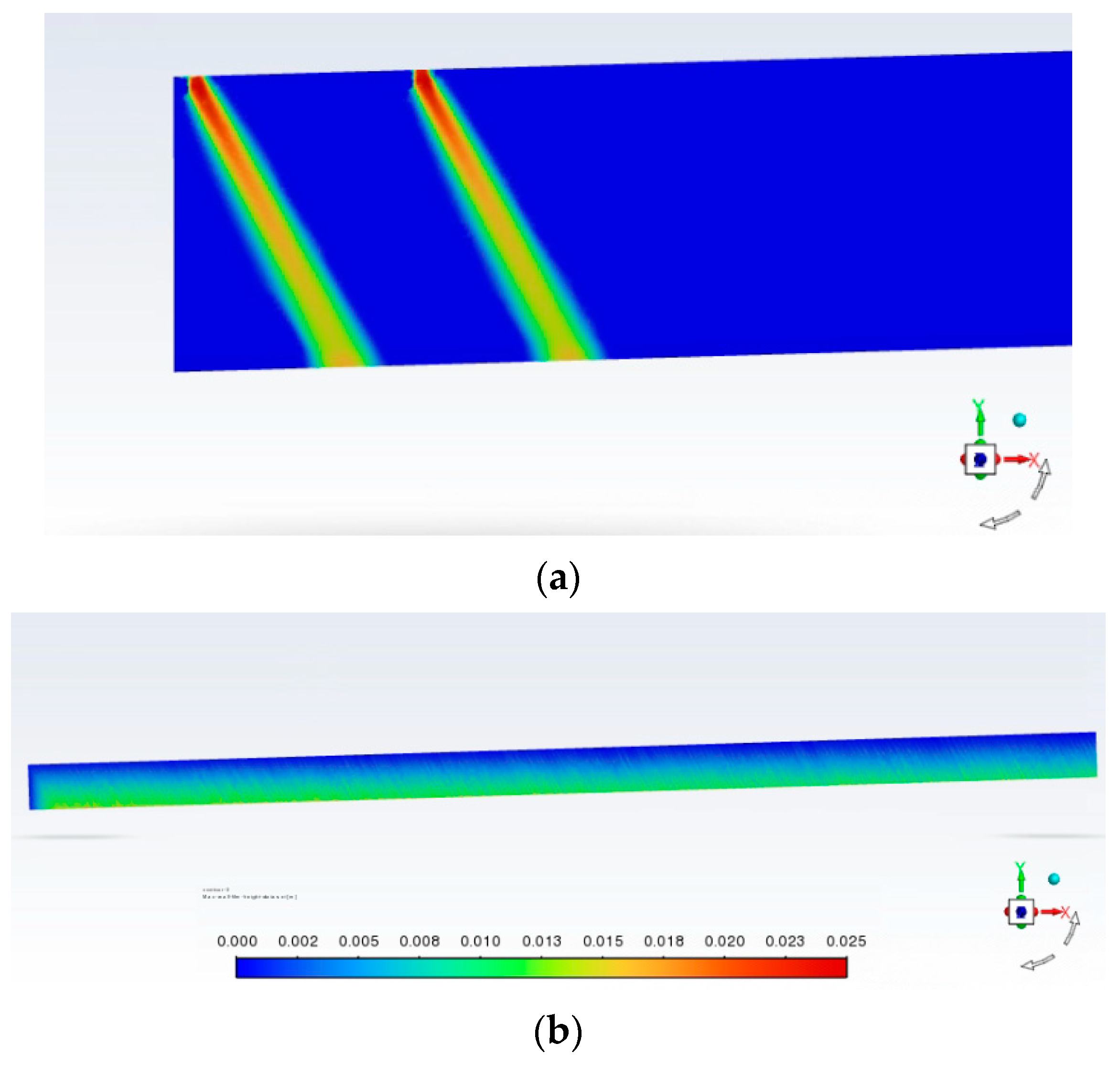
4.2.1. Distribution of the WFPL and WFD

Under the conditions of −1% LS and 2% TS, the WFPL and WFD distribution results of the two-way eight lanes of the circular-curve sections are shown in Figure 7. It can be seen that the direction of the WFP and the synthetic slope direction are similar. The WFD increases from the outside to the inside of the lane, with the maximum value distributed on the left curb. Preliminary conclusions can be drawn from the results of the above simulation: due to the presence of the TS in the outside of the circular-curve section, the water flows from the outer to the inner side of the pavement, and the WFD gradually decreases as the WFP moves away from the center.

4.2.2. Maximum Water Film Path Length (WFPLmax)

The WFPLmax of two-way eight-lane, ten-lane, and twelve-lane circular-curve sections are simulated under different linear combinations of TS and LS. The results are shown in Table 10. At a certain value of PW and TS, WFPLmax values are positively correlated with LS. With the arch TS is 2%, WFPL of 4% LS under two-way eight lanes is 2.21 times that of 0.3% LS. WFPL of 4% LS under two-way ten lanes is 2.21 times that of 2% LS. WFPL of 4% LS under two-way twelve lanes is 2.22 times that of 2% LS. The increase in LS, although allowing for an increase in the synthetic slope of the pavement, is biased in the direction of LS, while the longitudinal length of the pavement is quite long compared to the transverse width, which increases WFPL.
Increasing TS from 2% to 2.5% for circular-curved sections with the same LS can effectively reduce the WFPLmax. This not only increases the synthetic slope but also causes the synthetic LS direction to gradually deviate from the TS direction, which makes the WFPL decrease greatly because the transverse width of the pavement is quite short relative to the longitudinal length. When LS is the same, WFPLmax continues to become longer as PW becomes larger. This is due to certain conditions of the same TS and LS. The direction of water flowing is unchanged, and the number of lanes increases so that the PW increases. The water flow is correspondingly longer, so the WFPL increases greatly.
As shown in Table 11, it can be seen that when the number of lanes is certain, the larger the LS, the better the reduction effect of WFPLmax through changing TS from 2% to 2.5%. For a two-way eight-lane pavement, changing TS from 2% to 2.5%, the reduction of WFPLmax at 4% LS is 6.55 m, which is 82 times the decrease corresponding to 0.3% LS (0.08 m). For the two-way ten-lane pavement, changing TS from 2% to 2.5%, the reduction of WFPLmax at 4% LS is 7.86 m, which is 87 times the decrease in the corresponding 0.3% LS (0.09 m). For the two-way twelve-lane pavement, the reduction of WFPLmax at 4% LS is 9.17 m, which is 92 times the decrease corresponding to 0.3% LS. From Table 11, it can be found that the reduction of WFPLmax, when changing TS from 2% to 2.5%, is not only obvious with the increase in LS, but is significant with the increase in PW. It can be concluded that in the case of a wide circular-curve section with limited alignment and large design LS, it can be considered to increase TS from 2% to 2.5% to reduce WFPLmax, and the wider the pavement width, the better the improvement effect.
The following linear regression analysis was carried out using SPSS to rank the effect degree of the three indicators of TS, LS, and PW on WFPLmax regarding the absolute value of the standard coefficient, and the results are shown in Table 12. From Table 12, it can be seen that when using the absolute value of the standard coefficient for comparison, the LS has the greatest influence on the WFPLmax, followed by the PW, and the TS has the smallest influence.

4.2.3. Maximum Water Flow Depth (WFDmax)

Results of the WFDmax, the WFD on the first lane middle line, and the WFD on the second lane middle line of circular-curve sections under different LS, TS, and PW conditions at 120 km/h are shown in Table 13 and Table 14. For circular-curve sections under the design speed of 120 km/h, the WFDmax and the WFD on the first/second lane middle line are not greater than 5.03 mm, are lower than the safe WFD thresholds, thus meeting the needs of traffic safety. When PW and TS are certain, the WFDmax and WFD on the first/second lane middle line increase with the increase in LS. For two-way eight lanes under 2% TS and 4% LS, the WFDmax is 3.65 mm relative to a 2% LS increase of 0.14 mm. For two-way ten lanes under 2% TS and 4% LS, the WFDmax is 3.89 mm relative to the 2% LS increase of 0.14 mm. For the two-way ten lanes under 2% TS and 4% LS, the WFDmax is 4.12 mm relative to the 2% LS increase of 0.16 mm. This is because when the TS is fixed, the increase in LS makes the synthetic slope direction favor the longitudinal direction of the pavement, the WFPLmax becomes bigger, and the retention time of the water flow on the surface becomes longer, which leads to the increase in the WFD.
When the LS is the same, increasing the TS from 2% to 2.5% can effectively reduce the WFD. As the LS and PW increase, increasing the TS has a better effect on reducing the WFD. The increase in TS can not only increase the synthetic slope of the pavement and accelerate the water drainage but also make the direction of the WFP gradually biased in the direction of TS because the length of the transverse width of the pavement is much smaller than the length of the longitudinal direction, which makes the pavement surface water in a certain width of the pavement flow through a reduced distance, and the WFPL is shortened so that the WFD is greatly reduced. Moreover, the WFDmax and the WFD on the first and second lanes become larger as the PW increases at a certain TS and LS. This is due to the fact that as the number of lanes increases, the pavement becomes wider, the WFPLmax becomes longer, the corresponding WFPL also becomes longer, and the retention time of the surface water on the pavement becomes longer, resulting in the accumulation of water film, and the WFD increases accordingly.
The relationship between the change rate of the WFDmax and LS is shown in Figure 8. From Figure 8, it can be seen that when LS is certain, the change rate of the WFDmax (Figure 8a), the change rate of the WFD in the first travel lane middle (Figure 8b), and the change rate of the WFD in the second lane middle (Figure 8c) decrease successively, indicating that the further the distance from the central median, the smaller the change rate of the WFD affected by LS. Moreover, the change trends of the WFDmax and the WFDs in the first/second lanes with the growth of the LS are consistent, and all of them have the maximum value at LS of 2.1%. In cases where the LS is less than 2.1%, the WFD change rate becomes faster as LS increases, while in cases where the LS is greater than or equal to 2.1%, the WFD change rate becomes slower with the LS growth. In the case of LS between 1.1% and 4%, the change in LS has a greater effect on the WFD than in the case of LS between 0.3% and 1.1%. It can be concluded that it is more effective to reduce the WFD by adjusting LS when the LS is between 1.1–4%, and it is not recommended to prioritize adjusting the LS metrics to reduce the WFDmax when the LS is less than 1.1%.
Moreover, widening of two-way ten lanes to twelve lanes while adjusting TS from 2% to 2.5%, or widening of two-way eight lanes to ten lanes while adjusting TS from 2% to 2.5%, can both reduce the WFDmax, and the wider the pavement, the greater the magnitude of the reduction of the WFDmax. The maximum reduction can reach 0.08 mm. Therefore, in the design of the widening of the old road, 2.5% can be considered the minimum TS to effectively alleviate the problem of the WFD on the inside of the road becoming larger as a result of road widening.
The linear regression analysis was carried out using SPSS to rank the influence degree of the three indicators of the TS, LS, and PW on the WFDmax regarding the absolute value of the standard coefficient, and the results are shown in the table below. As can be seen from Table 15, when using the absolute value of the standard coefficients for comparison, PW has the greatest impact on WFDmax, followed by TS and LS.

5. Conclusions

Based on the simulation results and analysis of straight-line and circular-curve sections under different linear combination conditions, the following conclusions can be drawn:
  • According to the absolute values of Beta, the influence of each linear index on the WFPLmax and WFDmax for both straight-line and circular-curve sections is different: LS has the greatest influence on the WFPLmax, followed by the PW; while the PW has the greatest influence on the WFDmax, and LS has the least effect.
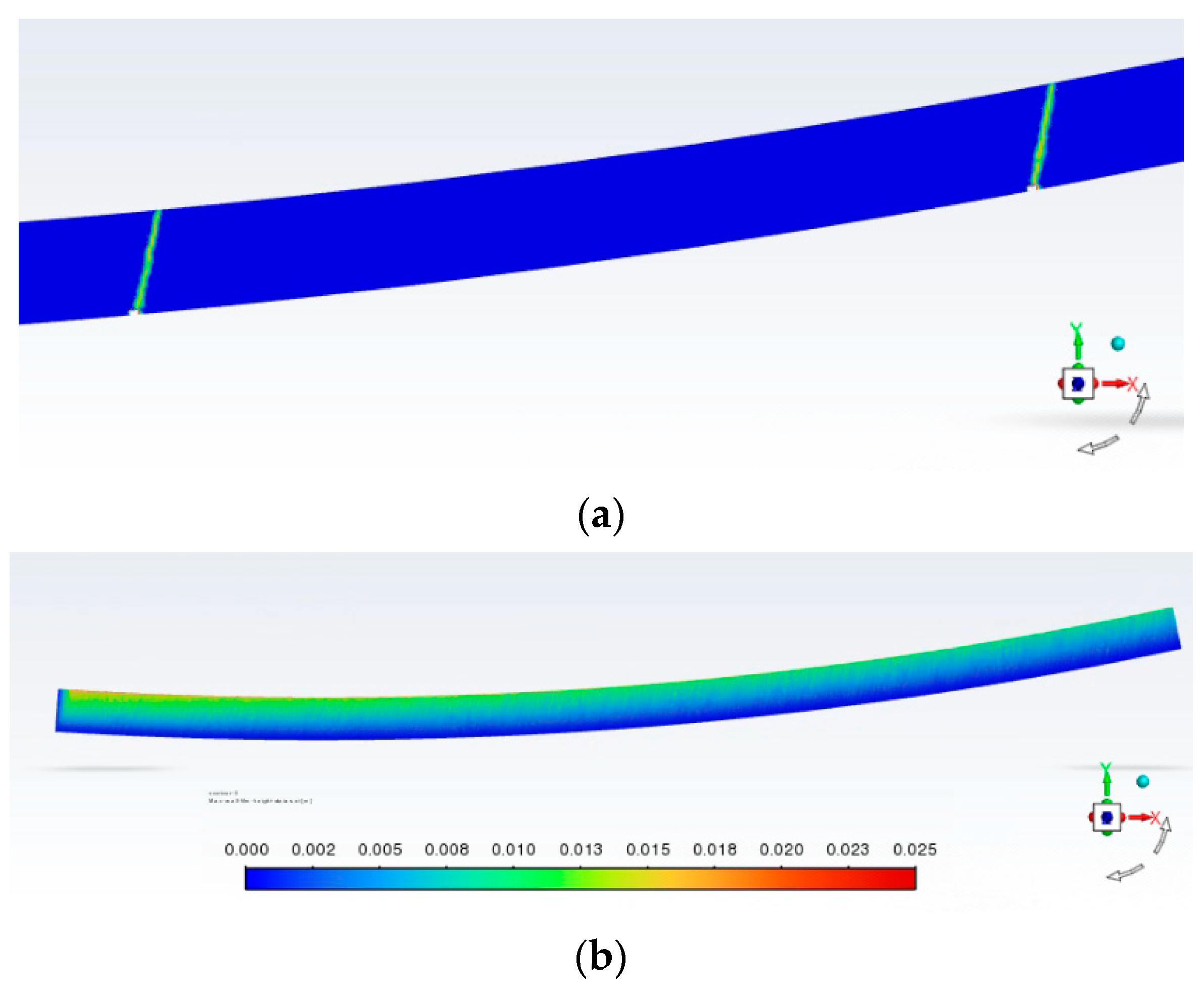
  • WFDmax is positively correlated with the WFPLmax, and the increase in the WFPL makes the retained time of water flow in the pavement longer, increasing the WFD. The WFD increases gradually along the direction of the WFPLmax and reaches the maximum value on the inside of the road curb.
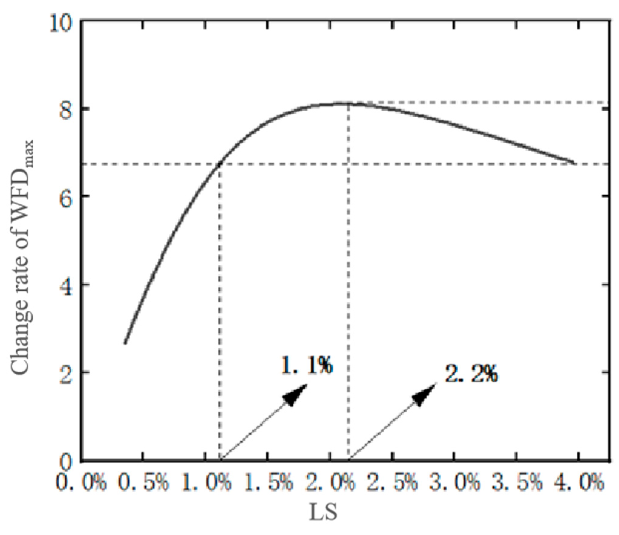
  • When the design value of LS is between 1.1% and 4%, the WFDmax can be effectively reduced by lowering the LS; and when the LS is less than 1.1%, it is not recommended to prioritize the adjustment of the LS to reduce the WFDmax.
  • In the case of large design values of the LS, it can be considered to effectively reduce the WFPLmax by increasing the arch TS from 2% to 2.5% for straight-line and circular-curve sections, and the wider PW, the better the improvement effect.
  • While the pavement width is widened, adjusting TS from 2% to 2.5% can effectively offset the increasing effect of the PW on the WFDmax.
Finally, this research aims to provide a better understanding of the runoff characteristics of wide expressway asphalt pavements. Future studies will be focused on the simulation of S-curve sections under different linear combination conditions, establishing a three-dimensional numerical model of a wide expressway asphalt pavement to simulate the rainfall catchment process and field validation.

Author Contributions

Conceptualization, Z.C., X.R. and H.Y.; Methodology, Z.C., Z.L., X.L., X.R. and H.Y.; Validation, Z.C., Z.L. and X.L.; Investigation, Z.L. and T.H.; Writing—original draft, Z.C. and Z.L.; Supervision, Z.C., X.R. and H.Y.; Funding acquisition, H.Y. All authors have read and agreed to the published version of the manuscript.

Funding

This research was funded by Guangdong Basic and Applied Basic Research Foundation (grant numbers 2022A1515011537, 2022A1515011607, and 2020A1515110900).

Data Availability Statement

The data presented in this study are available on request from the corresponding author. The data are not publicly available due to privacy.

Acknowledgments

The authors would like to thank the technicians at the Road laboratories of South China University of Technology for technical support and assistance in experimental activities.

Conflicts of Interest

Authors Zhenggang Cheng, Zhiyong Liang, Xuhua Li, Xiaowei Ren and Tao Hu were employed by the company Guangdong Province Communications Planning & Design Institute Co., Ltd. The remaining author declares that the research was conducted in the absence of any commercial or financial relationships that could be construed as a potential conflict of interest.

References

  1. Hermange, C.; Oger, G.; Le Chenadec, Y.; de Leffe, M.; Le Touzé, D. In-depth analysis of hydroplaning phenomenon accounting for tire wear on smooth ground. J. Fluids Struct. 2022, 111, 103555. [Google Scholar] [CrossRef]
  2. Spitzhüttl, F.; Goizet, F.; Unger, T.; Biesse, F. The real impact of full hydroplaning on driving safety. Accid. Anal. Prev. 2020, 138, 105458. [Google Scholar] [CrossRef] [PubMed]
  3. Huang, X.; Liu, X.; Cao, Q.; Yan, T.; Zhu, S.; Zhou, X. Numerical Simulation of Tire Partial Hydroplaning on Flooded Pavement. J. Hunan Univ. (Nat. Sci.) 2018, 45, 113–121. [Google Scholar]
  4. Xiao, K.; Hui, B.; Qu, X.; Wang, H.; Diab, A.; Cao, M. Asphalt pavement water film thickness detection and prediction model: A review. J. Traffic Transp. Eng. (Engl. Ed.) 2023, 10, 349–367. [Google Scholar] [CrossRef]
  5. Luo, W.; Li, L. Development of a new analytical water film depth (WFD) prediction model for asphalt pavement drainage evaluation. Constr. Build. Mater. 2019, 218, 530–542. [Google Scholar] [CrossRef]
  6. Ma, Y.; Geng, Y.; Chen, X.; Lu, Y. Prediction for asphalt pavement water film thickness based on artificial neural network. J. Southeast Univ. (Engl. Ed.) 2017, 33, 490–495. [Google Scholar]
  7. Lubnow, M.; Jeffries, J.B.; Dreier, T.; Schulz, C. Water film thickness imaging based on time-multiplexed near-infrared absorption. Opt. Express 2018, 26, 20902–20912. [Google Scholar] [CrossRef]
  8. Ling, J.; Yang, F.; Zhang, J.; Li, P.; Uddin, M.D.I.; Cao, T. Water-film depth assessment for pavements of roads and airport runways: A review. Constr. Build. Mater. 2023, 392, 132054. [Google Scholar] [CrossRef]
  9. Luo, W.; Li, L.; Wang, K.C.; Wei, C. Surface drainage evaluation of asphalt pavement using a new analytical water film depth model. Road Mater. Pavement Des. 2020, 21, 1985–2004. [Google Scholar] [CrossRef]
  10. Qi, Y. Effect of Road Alignment Combination on Pavement Runoff Characterisrics. Master’s Thesis, Southeast University, Nanjing, China, 2019. [Google Scholar]
  11. Akan, A.O. Drainage of Pavements Under Nonuniform Rainfall. J. Transp. Eng. 1986, 112, 172–183. [Google Scholar] [CrossRef]
  12. Jeong, J.; Charbeneau, R.J. Diffusion Wave Model for Simulating Storm-Water Runoff on Highway Pavement Surfaces at Superelevation Transition. J. Hydraul. Eng. 2010, 136, 770–778. [Google Scholar] [CrossRef]
  13. Charbeneau, R.J.; Jeong, J.; Barrett, M.E. Highway Drainage at Superelevation Transitions; The University of Texas at Austin: Austin, TX, USA, 2008. [Google Scholar]
  14. Liu, X.; Chen, Y.; Shen, C. Coupled Two-Dimensional Surface Flow and Three-Dimensional Subsurface Flow Modeling for Drainage of Permeable Road Pavement. J. Hydrol. Eng. 2016, 21, 04016051. [Google Scholar] [CrossRef]
  15. Softić, E.; Radičević, V.; Subotić, M.; Stević, Ž.; Talić, Z.; Pamučar, D. Sustainability of the Optimum Pavement Model of Reclaimed Asphalt from a Used Pavement Structure. Sustainability 2020, 12, 1912. [Google Scholar] [CrossRef]
  16. Luo, J.; Liu, J.; Wang, Y. Validation Test on Pavement Water Film Depth Prediction Model. China J. Highw. Transp. 2015, 28, 57–63. [Google Scholar]
  17. Zhang, L. The Water Sections Diagnosis and Control Techniques. Master’s Thesis, Chongqing Jiaotong University, Chongqing, China, 2013. [Google Scholar]
  18. Huebner, R.S.; Anderson, D.A.; Warner, J.C.; Reed, J.R. PAVDRN: Computer model for predicting water film thickness and potential for hydroplaning on new and reconditioned pavements. Transp. Res. Rec. 1997, 1599, 128–131. [Google Scholar] [CrossRef]
  19. Guo, S. Analysis on Pavement Runoff Characteristics of Super Multilane Expressway. North. Commun. 2021, 8, 64–68. [Google Scholar]
  20. Ji, T.; An, J.; He, S.; Li, C. Prediction of road Surface rainfall depth based on Artificial neural Network. Trans. Nanjing Univ. Aeronaut. Astronaut. 2006, 23, 115–119. [Google Scholar]
  21. Liu, Y.; Miao, H. Research on Performance of New Pavement Drainage System Under Rainfall Infiltration. China J. Highw. Transp. 2017, 30, 1–9. [Google Scholar]
  22. Escarameia, M.; Gasowski, Y.; May, R.W.P.; Bergamini, L. Estimation of runoff depths on paved areas. Urban Water J. 2006, 3, 185–197. [Google Scholar] [CrossRef]
  23. Pan, C.; Yu, P.; Lu, H. Numerical simulation of wetting and drying for shallow flows by Riemann solution on dry bed. J. Hydrodyn. 2009, 24, 305–312. [Google Scholar]
  24. Cea, L.; Garrido, M.; Puertas, J. Experimental validation of two-dimensional depth-averaged models for forecasting rainfall-runoff from precipitation data in urban areas. J. Hydrol. 2010, 382, 88–102. [Google Scholar] [CrossRef]
  25. Staufer, P.; Siekmann, M.; Loos, S.; Pinnekamp, J. Numerical Modeling of Water Levels on Pavements under Extreme Rainfall. J. Transp. Eng. 2012, 138, 732–740. [Google Scholar] [CrossRef]
  26. Li, H.; Kayhanian, M.; Harvey, J.T. Comparative field permeability measurement of permeable pavements using ASTM C1701 and NCAT permeameter methods. J. Environ. Manag. 2013, 118, 144–152. [Google Scholar] [CrossRef] [PubMed]
  27. Aureli, F.; Maranzoni, A.; Mignosa, P.; Ziveri, C. A weighted surface-depth gradient method for the numerical integration of the 2D shallow water equations with topography. Adv. Water Resour. 2008, 31, 962–974. [Google Scholar] [CrossRef]
  28. Costabile, P.; Costanzo, C.; Macchione, F. Performances and limitations of the diffusive approximation of the 2-d shallow water equations for flood simulation in urban and rural areas. Appl. Numer. Math. 2016, 116, 141–156. [Google Scholar] [CrossRef]
  29. Liu, S.-H.; Tai, W.; Fan, M.; Luo, Q.-S. Numerical simulation of atomization rainfall and the generated flow on a slope. J. Hydrodyn. 2012, 24, 273–279. [Google Scholar] [CrossRef]
  30. Ji, T.; Huang, X.; Liu, Q.; Tang, G. Prediction model of rain water depth on road surface. J. Traffic Transp. Eng. 2004, 4, 1–3. [Google Scholar]
  31. Gallaway, B.M.; Schiller, R.E.; Rose, J.G. The Effects of Rainfall Intensity, Pavement Cross Slope, Surface Texture, and Drainage Length on Pavement Water Depths; Texas A&M University: College Station, TX, USA, 1971. [Google Scholar]
  32. Wambold, J.C.; Henry, J.J.; Hegmon, R.R. Evaluation of pavement surface texture significance and measurement techniques. Wear 1982, 83, 351–368. [Google Scholar] [CrossRef]
  33. JTG D20-2017; Design Specification for Highway Alignment. People’s Communications Press: Beijing, China, 2017.
Figure 1. Detail of pavement surface model.
Buildings 14 00254 g001
Figure 2. Rainfall area.
Buildings 14 00254 g002
Figure 3. Pavement model.
Buildings 14 00254 g003
Figure 4. WFPL and WFD simulation results of straight-line sections without LS: (a) WFPL distribution; (b) WFD distribution.
Buildings 14 00254 g004
Figure 5. WFPL and WFD simulation results of straight-line sections with LS: (a) WFPL distribution; (b) WFD distribution.
Buildings 14 00254 g005
Figure 6. Change rate of the WFDmax vs. LS.
Buildings 14 00254 g006
Figure 7. WFPL and WFD simulation results of circular-curve sections: (a) WFPL distribution; (b) WFD distribution.
Buildings 14 00254 g007
Figure 8. The change rate results: (a) change rate of the WFDmax vs. the LS; (b) change rate of the WFD on the first lane middle vs. the LS; (c) change rate of the WFD on the second lane middle vs. the LS.
Buildings 14 00254 g008
Table 1. Hourly rainfall intensity and mean diameter of raindrop.
Rainfall Intensity (mm/h)Mean Diameter of a Raindrop (mm)Hourly Rainfall Intensity (mm/h)Mean Diameter of a Raindrop (mm)
0.250.75–1.0025.42.00–2.25
1.271.00–1.2550.82.25–2.75
2.541.25–1.50101.62.75–3.00
12.701.75–2.00152.43.00–3.25
Table 2. Linear combination conditions of straight-line sections.
Number of Lanes per SideSection Length (m)LS (%)TS (%)
4300−0.32
−0.5
5−1.0
−2.02.5
63.0
−4.0
Table 3. Linear combination condition of circular-curve sections.
Number of Lanes per SideSection Length (m)Radius of the Circular Curve (m)LS (%)TS (%)
43004500−0.3%2.0%
−0.5%
5−1.0%
−2.0%2.5%
6−3.0%
−4.0%
Table 4. WFPLmax (m) under different LS, TS, and PW conditions at 120 km/h.
Number of Lanes in Both Sides LS (%)0.30.51.02.03.04.0
TS (%)
82.015.9316.2317.6122.2728.3935.22
2.515.8616.0616.9620.1724.6029.72
102.019.7220.1021.8027.5835.1543.60
2.519.6419.8921.0024.9730.4636.79
122.023.5123.9725.9932.8841.9151.99
2.523.4223.7125.0429.7736.3243.87
Table 5. WFPLmax reduction (m) of TS from 2% to 2.5% for different number of lanes at 120 km/h.
Number of Lanes on
Both Sides
81012
LS (%)
0.30.070.080.09
45.506.818.12
Multiple788590
Table 6. Multiple regression model coefficient of WFPLmax.
ModelUnstandardized CoefficientStandard CoefficienttSignificanceCovariance Statistic
BStandard ErrorBetaToleranceVIF
Constant2.261.28/1.770.078//
LS−5.800.11−0.78−54.480.001.001.00
TS−6.230.46−0.20−13.560.001.001.00
PW1.460.0370.5638.940.001.001.00
Table 7. WFDmax (mm) under different LS, TS, and PW conditions at 120 km/h.
Number of Lanes on Both Sides LS (%)0.30.51.02.03.04.0
TS (%)
82.03.20 3.21 3.23 3.29 3.36 3.42
2.53.01 3.01 3.03 3.07 3.12 3.17
102.03.46 3.46 3.49 3.56 3.63 3.70
2.53.25 3.25 3.27 3.32 3.37 3.43
122.03.69 3.69 3.72 3.79 3.87 3.94
2.53.46 3.47 3.48 3.53 3.59 3.65
Table 8. WFD (mm) on the middle line of the first lane and the second lane under different LS, TS, and PW conditions at 120 km/h.
Number of Lanes on Both Sides LS (%)The First LaneThe Second Lane
TS (%) 0.30.51.02.03.04.00.30.51.02.03.04.0
82.01.671.681.691.731.761.802.312.312.332.382.422.47
2.51.571.581.591.601.641.662.162.172.192.222.252.28
102.01.681.681.681.731.751.802.322.322.332.382.432.47
2.51.581.591.591.611.651.672.172.182.192.222.252.29
122.01.671.681.691.731.761.812.312.322.332.392.442.47
2.51.581.591.591.611.651.682.172.192.192.222.262.29
Table 9. Multiple regression model coefficient of the WFDmax.
ModelUnstandardized CoefficientStandard CoefficienttSignificanceCovariance Statistic
BStandard ErrorBetaToleranceVIF
Constant3.190.011 284.300.00
LS−0.060.001−0.27−63.600.001.001.00
TS−0.480.004−0.50−119.310.001.001.00
PW0.060.0000.82194.940.001.001.00
Table 10. WFPLmax under different LS, TS, and PW conditions at 120 km/h.
Number of Lanes on Both Sides LS (%)0.30.51.02.03.04.0
TS (%)
82.018.9619.3320.9626.5233.8041.93
2.518.8819.1220.1924.0129.2935.38
102.022.7523.1925.1631.8240.5650.31
2.522.6622.9524.2328.8135.1542.45
122.026.5427.0629.3537.1247.3258.70
2.526.4426.7728.2733.6241.0049.53
Table 11. WFPLmax reduction (m) of TS from 2% to 2.5% for different number of lanes at 120 km/h.
Number of Lanes
on Both
Sides
81012
LS (%)
0.30.080.090.10
46.557.869.17
Multiple828792
Table 12. Multiple regression model coefficient of WFPLmax.
ModelUnstandardized CoefficientStandard CoefficienttSignificanceCovariance Statistic
BStandard ErrorBetaToleranceVIF
Constant7.371.47/5.010.00//
LS6.460.120.8255.30.001.001.00
TS−6.900.53−0.19−13.020.001.001.00
PW1.430.040.4933.030.001.001.00
Table 13. WFDmax (mm) under different LS, TS, and PW conditions at 120 km/h.
Number of Lanes on Both Sides LS (%)0.30.51.02.03.04.0
TS (%)
82.03.41 3.42 3.44 3.51 3.58 3.65
2.53.21 3.21 3.22 3.27 3.33 3.38
102.03.64 3.65 3.67 3.75 3.82 3.89
2.53.42 3.43 3.44 3.49 3.55 3.61
122.03.85 3.86 3.88 3.96 4.04 4.12
2.53.62 3.62 3.64 3.69 3.75 3.81
Table 14. WFT (mm) on the middle line of the first lane and the second lane under different LS, TS, and PW conditions at 120 km/h.
Number of Lanes on Both Sides LS (%)The First LaneThe Second Lane
TS (%) 0.30.51.02.03.04.00.30.51.02.03.04.0
82.03.233.243.263.323.393.453.233.243.263.323.393.45
2.53.043.043.053.103.153.203.043.043.053.103.153.20
102.03.483.493.513.583.663.723.483.493.513.583.663.72
2.53.273.283.293.343.403.453.273.283.293.343.403.45
122.03.713.713.743.813.893.963.713.713.743.813.893.96
2.53.483.493.503.563.613.673.483.493.503.563.613.67
Table 15. Multiple regression model coefficient of WFDmax.
ModelUnstandardized CoefficientStandard CoefficienttSignificanceCovariance Statistic
BStandard ErrorBetaToleranceVIF
Constant3.540.01/312.760.00//
LS0.060.000.3068.030.001.001.00
TS−0.510.00−0.55−123.730.001.001.00
Disclaimer/Publisher’s Note: The statements, opinions and data contained in all publications are solely those of the individual author(s) and contributor(s) and not of MDPI and/or the editor(s). MDPI and/or the editor(s) disclaim responsibility for any injury to people or property resulting from any ideas, methods, instructions or products referred to in the content.

