


A Comprehensive Approach to Earthquake-Resilient Infrastructure: Integrating Maintenance with Seismic Fragility Curves


Abstract
:1. Introduction
- : The uncertain damage state of a particular component, {0, 1, …};
- : A particular value of the DS;
- : The number of possible damage states;
- : Uncertain excitation, the ground-motion-intensity measure (i.e., PGA, PGD, or PGV);
- : A particular value of the IM;
- : The standard cumulative normal distribution function;
- : The median capacity of the component to resist a damage state ds measured in terms of the IM;
- : The logarithmic standard deviation of the uncertain capacity of the component to resist a damage state ds.
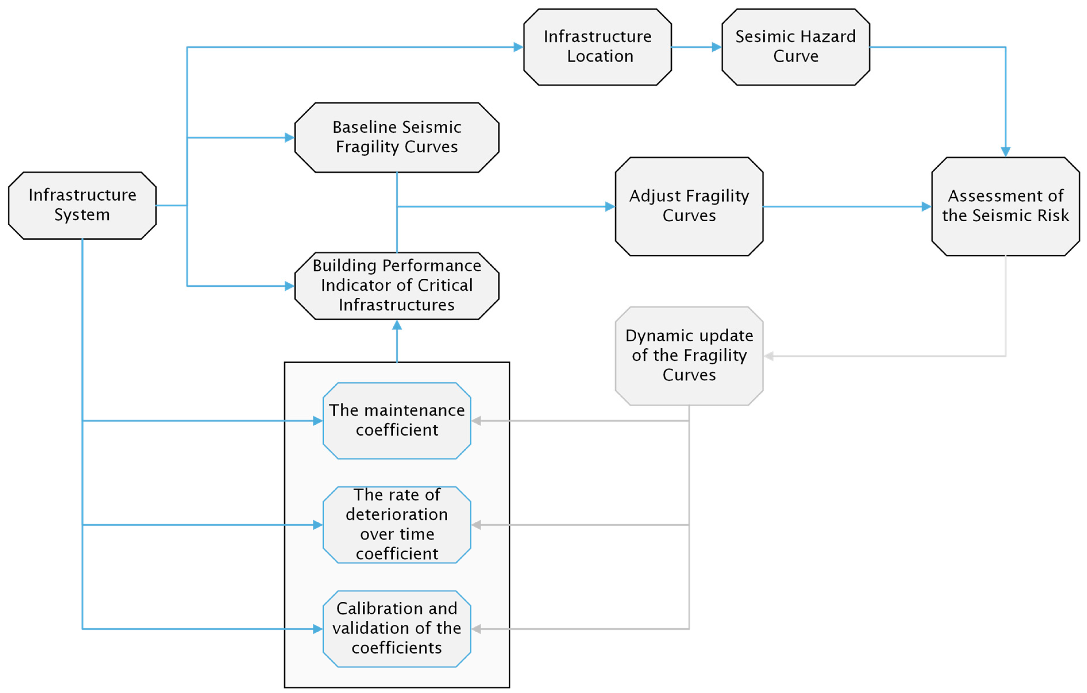
2. Integration of the Building Performance Indicator with Seismic Fragility Curves
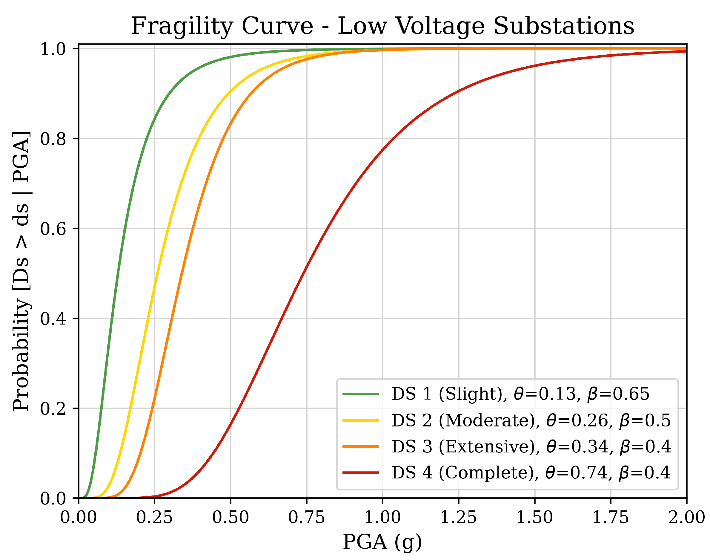
2.1. Baseline Seismic Fragility Curves
2.2. Building Performance Indicator of Critical Infrastructures
2.2.1. The Maintenance Coefficient
- Frequency of Maintenance: how regular maintenance activities are performed. Regular, scheduled maintenance usually indicates a higher maintenance level.
- Quality of Maintenance: the thoroughness and effectiveness of maintenance procedures. High-quality maintenance that addresses potential issues proactively contributes to a higher maintenance level.
- Maintenance History: past maintenance records, including any instances of delayed or skipped maintenance, which might impact the current condition of the component or system.
- Current Condition: the current physical condition of the component or system, assessed through inspections or condition-monitoring systems. This could include factors such as wear and tear, damage state, degradation, etc.
- Performance Metrics: operational data indicating the performance of the component or system. This might include efficiency, reliability, or failure rates, among other metrics.
- —Building Performance Indicator (0–100);
- —Performance level for system n (on a scale of 0 to 100);
- —Weight of system n in the BPI.
- BPI > 80 indicates that the state of the building and its resultant performance are good or better;
- 70 < BPI < 80 indicates that the state of the building is such that some of the systems are in marginal condition, i.e., some preventive maintenance measures must be taken;
- 60 < BPI < 70 indicates deterioration of the building, i.e., preventive and breakdown maintenance activities must be carried out;
- BPI < 60 means that the building is run-down.
2.2.2. The Rate of the Deterioration-over-Time Coefficient
- Age of the System: the period since the component or system was installed or last renovated. Older components typically show more signs of wear and tear.
- Designed Lifecycle: the lifecycle for which the component or system was initially designed also impacts its rate of deterioration. Components designed for a longer lifespan may have higher durability and slower deterioration compared to those designed for shorter lifecycles.
- Service regime: the degree and nature of usage can accelerate the deterioration process.
- Environmental Conditions: exposure to harsh environmental conditions, such as temperature fluctuations, humidity, salinity, etc., can influence the rate of deterioration.
- Material Properties: different construction materials have different inherent lifespans and susceptibility to deterioration. For instance, steel might corrode over time while concrete may experience spalling, cracking, and corrosion.
- : Service-regime-intensity factor;
- : Environmental-conditions factor;
- : Material-properties factor;
- : Weights associated with each factor;
- : Calibration coefficient for the performance score for perfect conditions;
- : Performance score of the infrastructure.
- : Deterioration-over-time coefficient at time t;
- : Time. The number of years since the start of the evaluation period;
- : Initial performance (usually set a 1.0);
- : Designed lifecycle of the infrastructure.
2.2.3. Integrating Uncertainty to the Model
2.2.4. Calibration and Validation of the Coefficients
2.3. Adjust Fragility Curves Based on the Maintenance Level and the Rate of Deterioration
2.4. Dynamic Update of the Fragility Curves
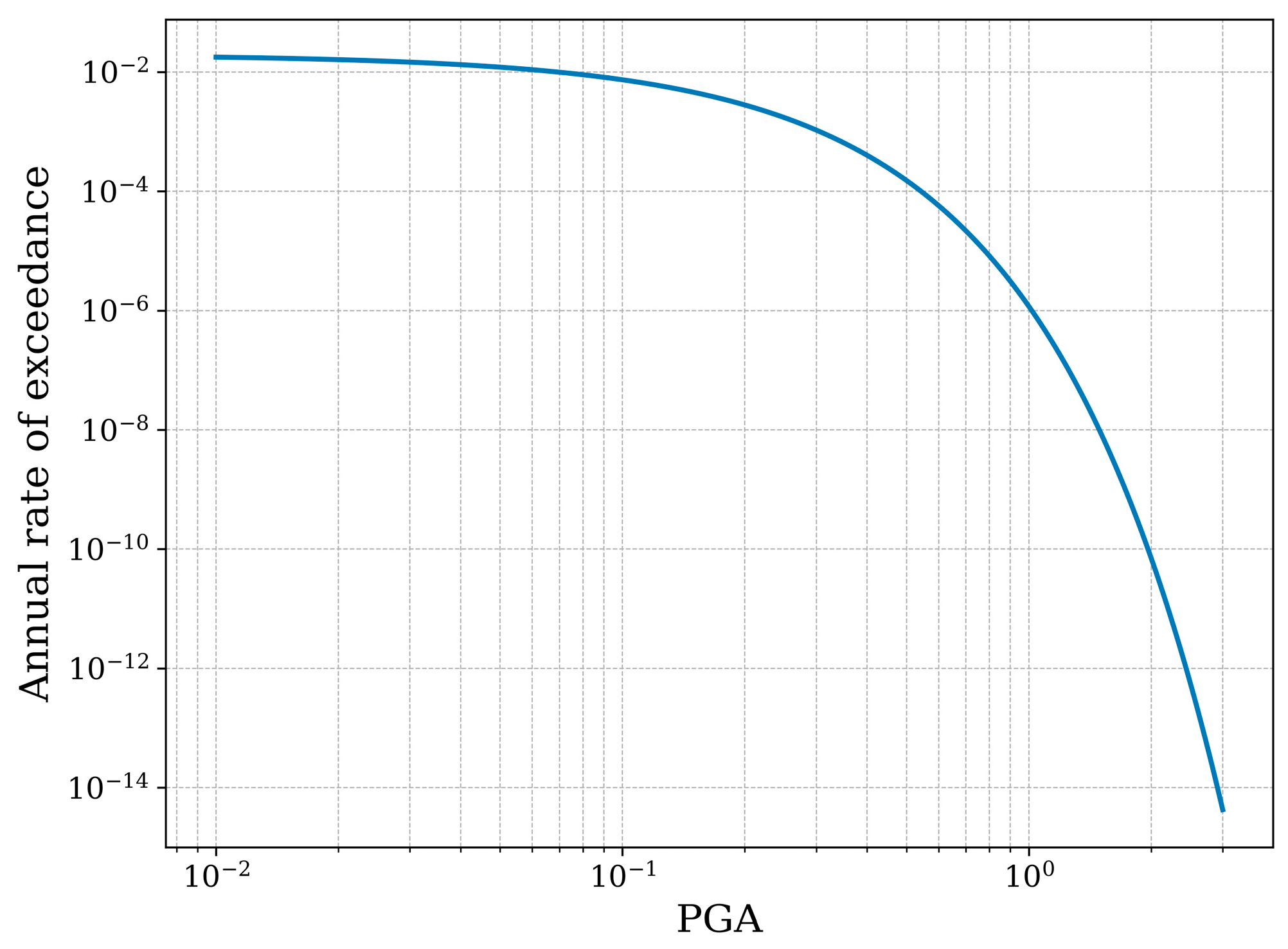
2.5. Assessment of the Seismic Risk
- —Total risk for the infrastructure design life cycle;
- —Damage rate of damage state i;
- —Conditional probability of being in a certain damage state for a given ;
- —Design lifecycle;
- —Annual rate of exceedance of a given ;
- —Repair cost (US$);
- —Direct loss (US$);
- —Indirect loss coefficient;
- —Overall consequences (US$).
3. Case Study
3.1. Baseline Seismic Fragility Curves
3.2. Analysis of Building Performance Coefficients
3.3. Risk Calculations
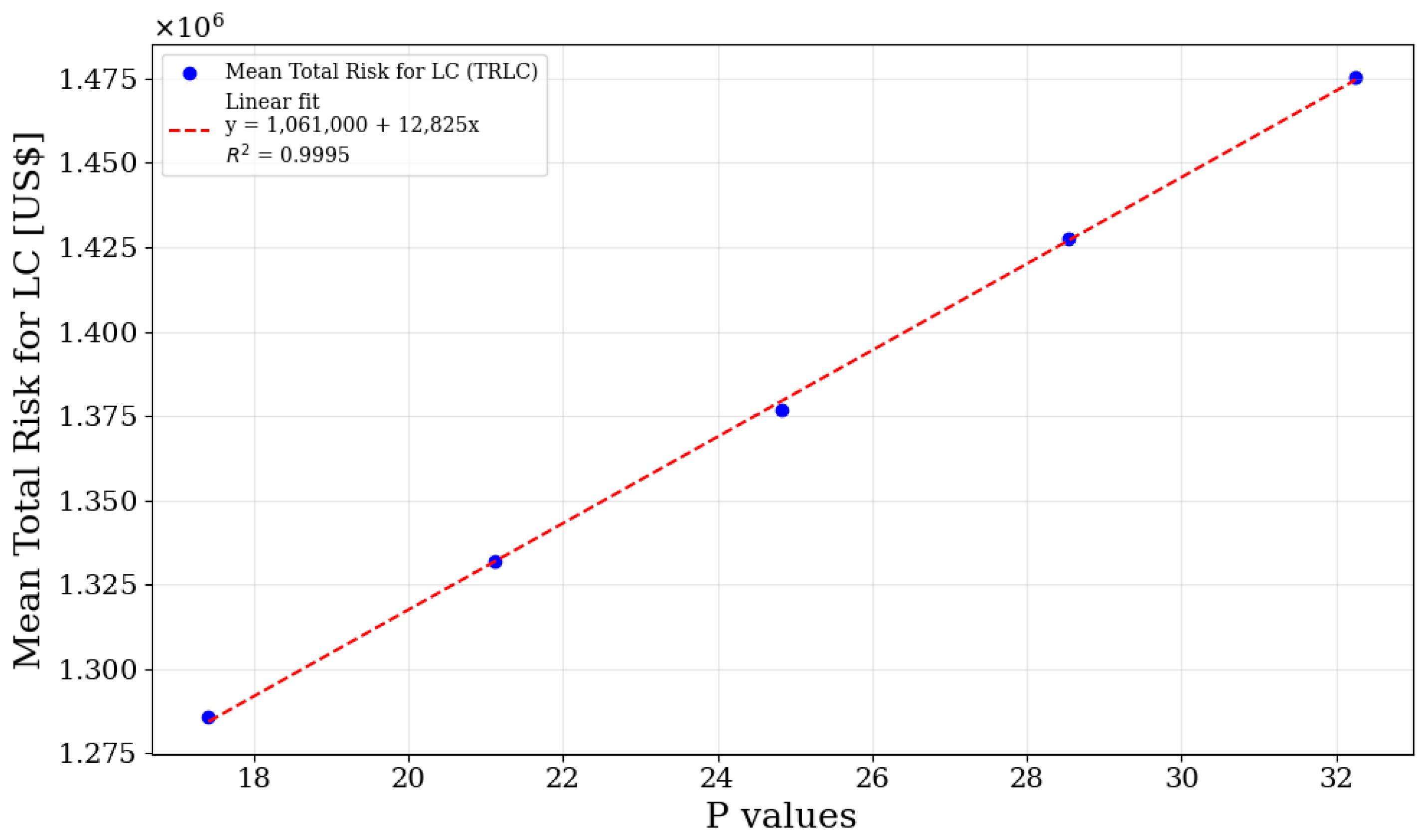
4. Sensitivity Analysis
5. Results and Discussion
6. Practical Applicability of the Research
- Decision-making for infrastructure maintenance—The framework provides a quantitative basis for making maintenance decisions. By considering not just the structural attributes but also the state of maintenance, decision-makers can allocate resources more efficiently, targeting the most vulnerable components for repair or upgrades.
- Seismic risk assessment—Integrating maintenance factors into seismic fragility curves allows for a more realistic and dynamic evaluation of seismic risks. This approach is precious for areas prone to seismic events, as it enhances preparedness and response strategies.
- Policy and Regulation—Our methodology can serve as a foundation for developing more comprehensive policies and regulations related to infrastructure resilience against seismic events. Regulatory bodies can adopt our study’s metrics and indicators for standardization.
- Economic efficiency—The proposed framework enables a more efficient allocation of resources by focusing on both maintenance and seismic resilience, potentially leading to significant cost savings in the long term.
7. Conclusions
8. Limitations
Author Contributions
Funding
Data Availability Statement
Conflicts of Interest
Appendix A. Classification and Grading of Service Regime, Environmental Conditions, and Material Properties
- Very-light service regime (e.g., a residential road)
- Light service regime (e.g., a small-town main road)
- Moderate service regime (e.g., a city street)
- Intensive service regime (e.g., a busy city street)
- Very-intensive service regime (e.g., a highway or freeway)
- Very-mild conditions (e.g., indoor, climate-controlled, stable temperature and humidity, no exposure to weather or environmental stressors such as extreme wind storms, no heat and tow cycles)
- Mild conditions (e.g., outdoor in a region with mild weather, moderate temperature and humidity, limited exposure to weather extremes)
- Moderate conditions (e.g., outdoor with some weather extremes, occasional exposure to high or low temperatures, humidity variations, or mild salinity)
- Harsh conditions (e.g., outdoor with regular weather extremes, frequent exposure to high or low temperatures, humidity variations, or moderate salinity)
- Very-harsh conditions (e.g., coastal areas with high salinity, areas with extreme temperatures or humidity, frequent exposure to severe weather conditions)
- Extremely durable materials (e.g., advanced composites)
- Durable materials (e.g., stainless steel, concrete)
- Moderately durable materials (e.g., steel)
- Less-durable materials (e.g., URM—unreinforced masonry wall)
- Highly susceptible to deterioration (e.g., wood, porose concrete)
References
- Urlainis, A.; Ornai, D.; Levy, R.; Vilnay, O.; Shohet, I.M. Loss and Damage Assessment in Critical Infrastructures Due to Extreme Events. Saf. Sci. 2022, 147, 105587. [Google Scholar] [CrossRef]
- Cinar, E.N.; Abbara, A.; Yilmaz, E. Earthquakes in Turkey and Syria-Collaboration Is Needed to Mitigate Longer Terms Risks to Health. BMJ 2023, 380, 559. [Google Scholar] [CrossRef] [PubMed]
- Gkougkoustamos, I.; Krassakis, P.; Kalogeropoulou, G.; Parcharidis, I. Correlation of Ground Deformation Induced by the 6 February 2023 M7.8 and M7.5 Earthquakes in Turkey Inferred by Sentinel-2 and Critical Exposure in Gaziantep and Kahramanmaraş Cities. GeoHazards 2023, 4, 267–285. [Google Scholar] [CrossRef]
- Cimellaro, G.P.; Reinhorn, A.M.; Bruneau, M. Framework for Analytical Quantification of Disaster Resilience. Eng. Struct. 2010, 32, 3639–3649. [Google Scholar] [CrossRef]
- Rasulo, A.; Pelle, A.; Briseghella, B.; Nuti, C. A Resilience-Based Model for the Seismic Assessment of the Functionality of Road Networks Affected by Bridge Damage and Restoration. Infrastructures 2021, 6, 112. [Google Scholar] [CrossRef]
- Bocchini, P.; Frangopol, D.M.; Ummenhofer, T.; Zinke, T. Resilience and Sustainability of Civil Infrastructure: Toward a Unified Approach. J. Infrastruct. Syst. 2014, 20, 04014004. [Google Scholar] [CrossRef]
- Porter, K. A Beginner’s Guide to Fragility, Vulnerability, and Risk; Springer: Berlin/Heidelberg, Germany, 2020. [Google Scholar]
- National Institute of Building Sciences. HAZUS-MH: Users’s Manual and Technical Manuals. In Report Prepared for the Federal Emergency Management Agency; Federal Emergency Management Agency: Washington, DC, USA, 2004. [Google Scholar]
- Urlainis, A.; Shohet, I.M. Development of Exclusive Seismic Fragility Curves for Critical Infrastructure: An Oil Pumping Station Case Study. Buildings 2022, 12, 842. [Google Scholar] [CrossRef]
- Porter, K.; Kennedy, R.; Bachman, R. Creating Fragility Functions for Performance-Based Earthquake Engineering. Earthq. Spectra 2007, 23, 471–489. [Google Scholar] [CrossRef]
- Porter, K.; Hamburger, R.; Kennedy, R. Practical Development and Application of Fragility Functions. In Proceedings of the Research Frontiers at Structures Congress 2007, Long Beach, CA, USA, 20 June 2007; American Society of Civil Engineers: Long Beach, CA, USA, 2007. [Google Scholar]
- Baker, J.W. Efficient Analytical Fragility Function Fitting Using Dynamic Structural Analysis. Earthq. Spectra 2015, 31, 579–599. [Google Scholar] [CrossRef]
- Sandoli, A.; Calderoni, B.; Lignola, G.P.; Prota, A. Seismic Vulnerability Assessment of Minor Italian Urban Centres: Development of Urban Fragility Curves. Bull. Earthq. Eng. 2022, 20, 5017–5046. [Google Scholar] [CrossRef]
- Rosti, A.; Rota, M.; Penna, A. Empirical Fragility Curves for Italian URM Buildings. Bull. Earthq. Eng. 2021, 19, 3057–3076. [Google Scholar] [CrossRef]
- Rosti, A.; Del Gaudio, C.; Rota, M.; Ricci, P.; Di Ludovico, M.; Penna, A.; Verderame, G.M. Empirical Fragility Curves for Italian Residential RC Buildings. Bull. Earthq. Eng. 2021, 19, 3165–3183. [Google Scholar] [CrossRef]
- Ruggieri, S.; Tosto, C.; Rosati, G.; Uva, G.; Ferro, G.A. Seismic Vulnerability Analysis of Masonry Churches in Piemonte after 2003 Valle Scrivia Earthquake: Post-Event Screening and Situation 17 Years Later. Int. J. Archit. Herit. 2020, 16, 717–745. [Google Scholar] [CrossRef]
- Rojas-Mercedes, N.; Erazo, K.; Di Sarno, L. Seismic Fragility Curves for a Concrete Bridge Using Structural Health Monitoring and Digital Twins. Earthq. Struct. 2022, 22, 503–515. [Google Scholar] [CrossRef]
- O’Rourke, M.J.; So, P. Seismic Fragility Curves for On-Grade Steel Tanks. Earthq. Spectra 2000, 16, 801–815. [Google Scholar] [CrossRef]
- Razzaghi, M.S.; Eshghi, S. Development of Analytical Fragility Curves for Cylindrical Steel Oil Tanks. In Proceedings of the 14th World Conference on Earthquake Engineering, Beijing, China, 12–17 October 2008; p. 8. [Google Scholar]
- Buratti, N.; Tavano, M. Dynamic Buckling and Seismic Fragility of Anchored Steel Tanks by the Added Mass Method. Earthq. Eng. Struct. Dyn. 2014, 43, 1–21. [Google Scholar] [CrossRef]
- Tseng, C.Y.; Wang, C.H.; Zheng, X.Y.; Chiu, H.C.; Jiang, J.A. Design of a Seismic Hazard Risk Assessment Model for EHV Transmission Grid. In Proceedings of the Second EAI International Conference, SmartGIFT 2017, London, UK, 27–28 March 2017. [Google Scholar] [CrossRef]
- Nariman, A.; Fattahi, M.H.; Talebbeydokhti, N.; Sadeghian, M.S. Assessment of Seismic Resilience in Urban Water Distribution Network Considering Hydraulic Indices. Iran. J. Sci. Technol. Trans. Civ. Eng. 2022, 47, 1165–1179. [Google Scholar] [CrossRef]
- Argyroudis, S.; Mitoulis, S.; Kaynia, A.M.; Winter, M.G. Fragility Assessment of Transportation Infrastructure Systems Subjected to Earthquakes. In Proceedings of the GEESD V, Geotechnical Special Publication (GSP 292), Austin, TX, USA, 10–13 June 2018. [Google Scholar] [CrossRef]
- Sevieri, G.; De Falco, A.; Marmo, G. Shedding Light on the Effect of Uncertainties in the Seismic Fragility Analysis of Existing Concrete Dams. Infrastructures 2020, 5, 22. [Google Scholar] [CrossRef]
- Frangopol, D.M.; Saydam, D.; Kim, S. Maintenance, Management, Lifecycle Design and Performance of Structures and Infrastructures: A Brief Review. Struct. Infrastruct. Eng. 2012, 8, 1–25. [Google Scholar] [CrossRef]
- Soleimanmeigouni, I.; Ahmadi, A.; Kumar, U. Track Geometry Degradation and Maintenance Modelling: A Review. Proc. Inst. Mech. Eng. Part F 2018, 232, 73–102. [Google Scholar] [CrossRef]
- Sedghi, M.; Kauppila, O.; Bergquist, B.; Vanhatalo, E.; Kulahci, M. A Taxonomy of Railway Track Maintenance Planning and Scheduling: A Review and Research Trends. Reliab. Eng. Syst. Saf. 2021, 215, 107827. [Google Scholar] [CrossRef]
- Volovski, M.; Murillo-Hoyos, J.; Saeed, T.U.; Labi, S. Estimation of Routine Maintenance Expenditures for Highway Pavement Segments: Accounting for Heterogeneity Using Random-Effects Models. J. Transp. Eng. Part A 2017, 143, 04017006. [Google Scholar] [CrossRef]
- Woldemariam, W.; Murillo-Hoyos, J.; Labi, S. Estimating Annual Maintenance Expenditures for Infrastructure: Artificial Neural Network Approach. J. Infrastruct. Syst. 2016, 22, 04015025. [Google Scholar] [CrossRef]
- Verdezoto, N.; Bagalkot, N.; Akbar, S.Z.; Sharma, S.; MacKintosh, N.; Harrington, D.; Griffiths, P. The Invisible Work of Maintenance in Community Health: Challenges and Opportunities for Digital Health to Support Frontline Health Workers in Karnataka, South India. Proc. ACM Hum.-Comput. Interact. 2021, 5, 1–31. [Google Scholar] [CrossRef]
- Caldera, S.; Mostafa, S.; Desha, C.; Mohamed, S. Integrating Disaster Management Planning into Road Infrastructure Asset Management. Infrastruct. Asset Manag. 2021, 8, 219–233. [Google Scholar] [CrossRef]
- Lei, X.; Sun, L.; Xia, Y. Seismic Fragility Assessment and Maintenance Management on Regional Bridges Using Bayesian Multi-Parameter Estimation. Bull. Earthq. Eng. 2021, 19, 6693–6717. [Google Scholar] [CrossRef]
- Zanini, M.A.; Faleschini, F.; Pellegrino, C. Cost Analysis for Maintenance and Seismic Retrofit of Existing Bridges. Struct. Infrastruct. Eng. 2016, 12, 1411–1427. [Google Scholar] [CrossRef]
- Shohet, I.M. Building Evaluation Methodology for Setting Maintenance Priorities in Hospital Buildings. Constr. Manag. Econ. 2003, 21, 681–692. [Google Scholar] [CrossRef]
- Manos, G.C.; Simos, N.; Kozikopoulos, E. The Structural Performance of Stone-Masonry Bridges. In Structural Bridge Engineering; IntechOpen: London, UK, 2016. [Google Scholar] [CrossRef]
- Crespi, P.; Zucca, M.; Valente, M.; Longarini, N. Influence of Corrosion Effects on the Seismic Capacity of Existing RC Bridges. Eng. Fail. Anal. 2022, 140, 106546. [Google Scholar] [CrossRef]
- Zanini, M.A.; Pellegrino, C.; Morbin, R.; Modena, C. Seismic Vulnerability of Bridges in Transport Networks Subjected to Environmental Deterioration. Bull. Earthq. Eng. 2013, 11, 561–579. [Google Scholar] [CrossRef]
- Soltani, M.; Raissi Dehkordi, M.; Eghbali, M.; Samadian, D.; Salmanmohajer, H. Influence of Infill Walls on Resilience Index of RC Schools Using the BIM Analysis and FEMA P-58 Methodology. Int. J. Civ. Eng. 2022, 21, 711–726. [Google Scholar] [CrossRef]
- Tecchio, G.; Donà, M.; Saler, E.; da Porto, F. Fragility of Single-Span Masonry Arch Bridges Accounting for Deterioration and Damage Effects. Eur. J. Environ. Civ. Eng. 2022, 27, 2048–2069. [Google Scholar] [CrossRef]
- Wang, K.C.; Almassy, R.; Wei, H.H.; Shohet, I.M. Integrated Building Maintenance and Safety Framework: Educational and Public Facilities Case Study. Buildings 2022, 12, 770. [Google Scholar] [CrossRef]
- Urlainis, A.; Shohet, I.M. Probabilistic Risk Appraisal and Mitigation of Critical Infrastructures for Seismic Extreme Events. In Proceedings of the Creative Construction Conference (CCC2018), Ljubljana, Slovenia, 30 June–3 July 2018. [Google Scholar] [CrossRef]
- Urlainis, A.; Shohet, I.M. Seismic Risk Mitigation and Management for Critical Infrastructures Using an RMIR Indicator. Buildings 2022, 12, 1748. [Google Scholar] [CrossRef]
- Wei, H.H.; Skibniewski, M.J.; Shohet, I.M.; Shapira, S.; Aharonson-Daniel, L.; Levi, T.; Salamon, A.; Levy, R.; Levi, O. Benefit-Cost Analysis of the Seismic Risk Mitigation for a Region with Moderate Seismicity: The Case of Tiberias, Israel. Procedia Eng. 2014, 85, 536–542. [Google Scholar] [CrossRef]
- Nuti, C.; Rasulo, A.; Vanzi, I. Seismic Safety Evaluation of Electric Power Supply at Urban Level. Earthq. Eng. Struct. Dyn. 2007, 36, 536–542. [Google Scholar] [CrossRef]
- Nuti, C.; Rasulo, A.; Vanzi, I. Seismic Safety of Network Structures and Infrastructures. Struct. Infrastruct. Eng. 2010, 6, 95–110. [Google Scholar] [CrossRef]
- Rasulo, A.; Nardoianni, S.; Evangelisti, A.; D’Apuzzo, M. Incorporating Traffic Models into Seismic Damage Analysis of Bridge Road Networks: A Case Study in Central Italy. Infrastructures 2023, 8, 113. [Google Scholar] [CrossRef]
- Federal Emergency Management Agency. Seismic Performance Assessment of Buildings—FEMA P-58; Federal Emergency Management Agency: Washington, DC, USA, 2012.
- Mitelman, A.; Lifshitz Sherzer, G. Coupling Numerical Modeling and Machine-Learning for Back Analysis of Cantilever Retaining Wall Failure. Comput. Concr. 2023, 31, 307–314. [Google Scholar] [CrossRef]
- Mitelman, A.; Yang, B.; Urlainis, A.; Elmo, D. Coupling Geotechnical Numerical Analysis with Machine Learning for Observational Method Projects. Geosciences 2023, 13, 196. [Google Scholar] [CrossRef]
- Mitelman, A.; Urlainis, A. Investigation of Transfer Learning for Tunnel Support Design. Mathematics 2023, 11, 1623. [Google Scholar] [CrossRef]
- Dabiri, H.; Faramarzi, A.; Dall’Asta, A.; Tondi, E.; Micozzi, F. A Machine Learning-Based Analysis for Predicting Fragility Curve Parameters of Buildings. J. Build. Eng. 2022, 62, 105367. [Google Scholar] [CrossRef]
- National Institute of Building Sciences. Hazus Earthquake Model Technical Manual Hazus 4.2 SP3; National Institute of Building Sciences: Washington, DC, USA, 2020. [Google Scholar]
- Klar, A.; Meirova, T.; Zaslavsky, Y.; Shapira, A. Spectral Acceleration Maps for Use in SI 413 Amendment No.5; The Geophysical Institute of Israel: Jerusalem, Israel, 2011. [Google Scholar]


| Damage State | Damage Ratio | |||
|---|---|---|---|---|
| DS1 | Slight | 0.13 | 0.65 | 0.05 |
| DS2 | Moderate | 0.26 | 0.50 | 0.11 |
| DS3 | Extensive | 0.34 | 0.40 | 0.55 |
| DS4 | Complete | 0.74 | 0.40 | 1 |
| Damage State | Description | |
|---|---|---|
| DS1 | Slight | Failure of 5% of the disconnect switches or circuit breakers, or by the building being in the slight damage state |
| DS2 | Moderate | Failure of 40% of disconnect switches, circuit breakers, or current transformers, or by the building being in the moderate damage state |
| DS3 | Extensive | Failure of 70% of disconnect switches, circuit breakers, current transformers, or transformers, or by the building being in the extensive damage state |
| DS4 | Complete | Failure of all disconnect switches, all circuit breakers, all transformers, or all current transformers, or by the building being in the complete damage state |
| System | Jan-17 | Jan-19 | Jan-21 | Apr-22 | Jul-22 | Oct-22 | Feb-23 |
|---|---|---|---|---|---|---|---|
| Structure | 80.0 | 88.0 | 90.0 | 90.0 | 90.0 | 90.0 | 90.0 |
| Exterior Envelope | 80.7 | 89.3 | 82.2 | 82.2 | 87.0 | 87.0 | 90.0 |
| Interior Finishes | 86.2 | 86.2 | 86.2 | 83.7 | 84.7 | 84.7 | 86.7 |
| Power Supply | 87.1 | 84.0 | 86.2 | 86.2 | 86.2 | 86.2 | 88.0 |
| Water and Sewerage System | 70.0 | 70.0 | 70.0 | 70.0 | 80.2 | 85.0 | 85.0 |
| HVAC | 64.8 | 70.0 | 90.0 | 90.0 | 90.0 | 90.0 | 90.0 |
| Fire Detection and Suppression | 95.0 | 95.0 | 90.0 | 90.0 | 90.0 | 87.0 | 90.0 |
| Elevators and Escalators | - | - | - | - | - | - | - |
| Peripheral Infrastructure | 90.0 | 82.5 | 67.5 | 67.5 | 75.0 | 75.0 | 75.0 |
| BPI Score | 84.0 | 83.3 | 85.3 | 84.5 | 86.5 | 86.8 | 88.1 |
| P | BPI | TRLC (US$) | |
|---|---|---|---|
| Mean | 21.05 | 85.45 | 1,330,458 |
| Std. | 4.23 | 1.57 | 50,953 |
| Min Value | 10.55 | 80.03 | 1,205,265 |
| 25% (1st Quartile) | 17.89 | 84.39 | 1,292,154 |
| 50% (Median) | 20.81 | 85.35 | 1,327,313 |
| 75% (3rd Quartile) | 23.75 | 86.49 | 1,362,107 |
| Max Value | 38.13 | 90.27 | 1,543,828 |
| Mean BPI | BPI = 75 | BPI = 80 | BPI = 85 | BPI = 90 | BPI = 95 |
|---|---|---|---|---|---|
| n= | 500 | 500 | 400,500 | 500 | 500 |
| Mean | 1,450,061 | 1,359,205 | 1,276,655 | 1,219,459 | 1,170,639 |
| Std. | 62,848 | 57,358 | 59,670 | 51,481 | 51,742 |
| min. | 1,271,963 | 1,184,940 | 1,135,168 | 1,061,887 | 1,059,202 |
| 25% | 1,407,262 | 1,318,910 | 1,234,882 | 1,184,530 | 1,135,560 |
| 50% | 1,443,205 | 1,355,042 | 1,274,359 | 1,214,930 | 1,166,577 |
| 75% | 1,490,181 | 1,398,849 | 1,316,040 | 1,251,680 | 1,201,536 |
| max. | 1,645,999 | 1,531,222 | 1,514,449 | 1,391,572 | 1,360,661 |
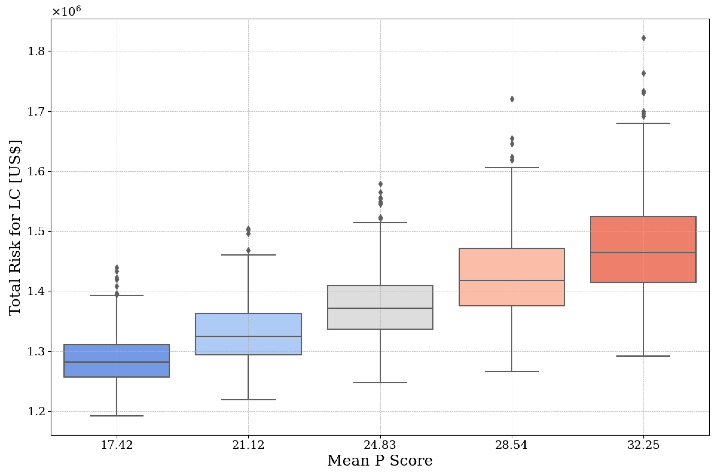
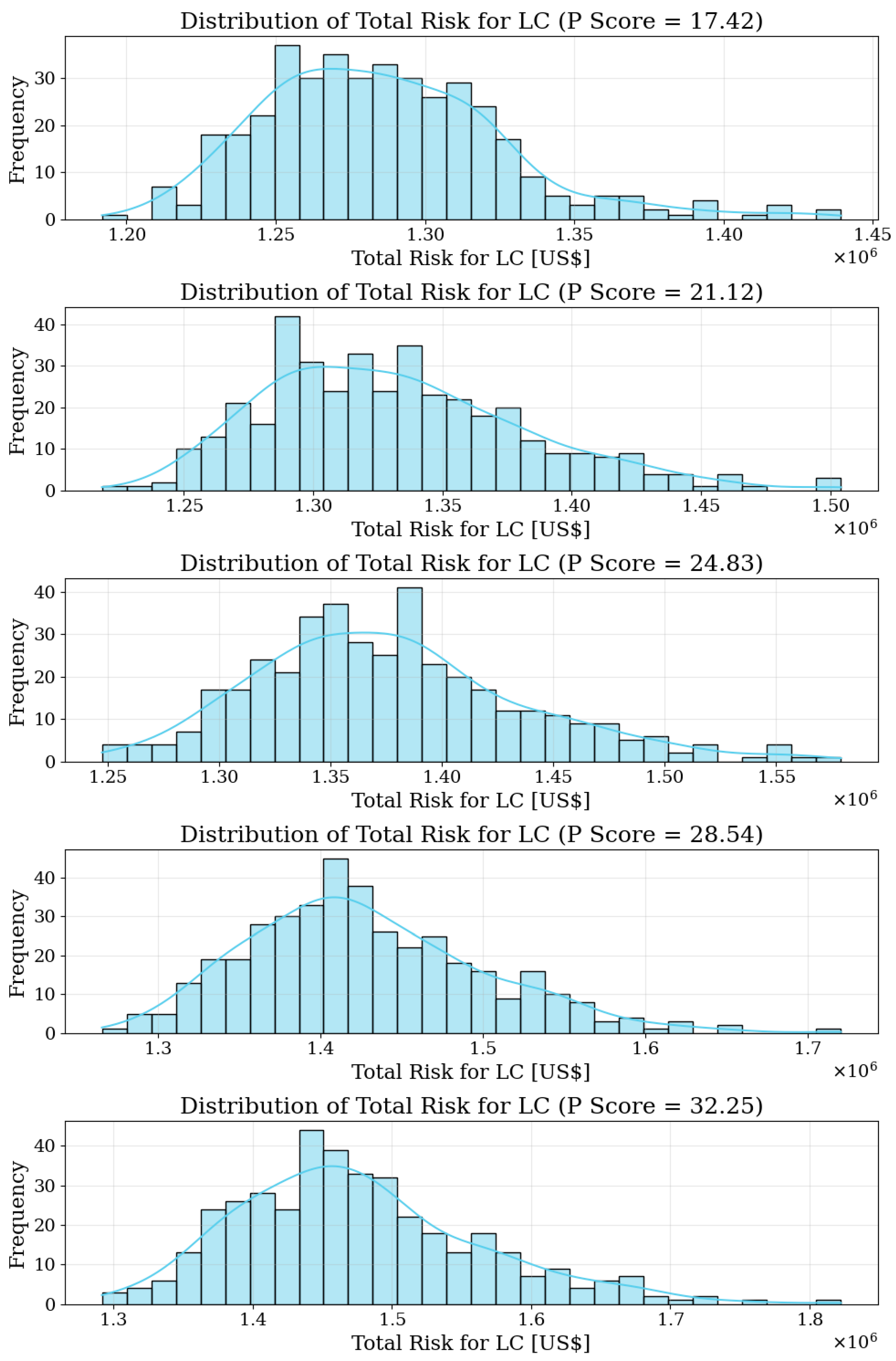
| Mean P | P = 17.42 | P = 21.13 | P = 24.83 | P = 28.54 | P = 32.25 |
|---|---|---|---|---|---|
| n= | 400 | 400 | 400 | 400 | 400 |
| Mean | 1,285,687 | 1,331,761 | 1,376,718 | 1,427,703 | 1,475,491 |
| Std. | 40,487 | 50,175 | 60,222 | 72,433 | 87,367 |
| min. | 1,191,755 | 1,218,358 | 1,247,397 | 1,265,752 | 1,291,696 |
| 25% | 1,256,330 | 1,293,241 | 1,336,244 | 1,375,846 | 1,414,411 |
| 50% | 1,281,857 | 1,324,765 | 1,371,375 | 1,417,702 | 1,464,657 |
| 75% | 1,310,973 | 1,362,096 | 1,409,387 | 1,471,124 | 1,524,204 |
| 99% | 1,419,327 | 1,460,045 | 1,549,155 | 1,619,376 | 1,699,655 |
| max. | 1,439,320 | 1,504,185 | 1,579,054 | 1,720,524 | 1,822,565 |
Disclaimer/Publisher’s Note: The statements, opinions and data contained in all publications are solely those of the individual author(s) and contributor(s) and not of MDPI and/or the editor(s). MDPI and/or the editor(s) disclaim responsibility for any injury to people or property resulting from any ideas, methods, instructions or products referred to in the content. |
© 2023 by the authors. Licensee MDPI, Basel, Switzerland. This article is an open access article distributed under the terms and conditions of the Creative Commons Attribution (CC BY) license (https://creativecommons.org/licenses/by/4.0/).
Share and Cite
Urlainis, A.; Shohet, I.M. A Comprehensive Approach to Earthquake-Resilient Infrastructure: Integrating Maintenance with Seismic Fragility Curves. Buildings 2023, 13, 2265. https://doi.org/10.3390/buildings13092265
Urlainis A, Shohet IM. A Comprehensive Approach to Earthquake-Resilient Infrastructure: Integrating Maintenance with Seismic Fragility Curves. Buildings. 2023; 13(9):2265. https://doi.org/10.3390/buildings13092265
Chicago/Turabian StyleUrlainis, Alon, and Igal M. Shohet. 2023. "A Comprehensive Approach to Earthquake-Resilient Infrastructure: Integrating Maintenance with Seismic Fragility Curves" Buildings 13, no. 9: 2265. https://doi.org/10.3390/buildings13092265
APA StyleUrlainis, A., & Shohet, I. M. (2023). A Comprehensive Approach to Earthquake-Resilient Infrastructure: Integrating Maintenance with Seismic Fragility Curves. Buildings, 13(9), 2265. https://doi.org/10.3390/buildings13092265