Abstract
Rapid urbanization and an increasing carbon footprint have underscored the need for sustainable practices in the construction industry. With the aim of prioritizing global sustainable development, the measurement of carbon emission efficiency in the construction industry (CEECI) has emerged as a critical indicator. Nevertheless, a comprehensive exploration of carbon emission efficiency within the Chinese construction sector remains limited, despite the pressing demand to mitigate carbon emissions. To address this research gap, this study aims to provide valuable policy recommendations for effectively reducing carbon emissions. We conducted a thorough assessment of both the total carbon emissions and the carbon emission intensity in 30 provinces and cities across China from 2010 to 2020. Utilizing the slacks-based measure (SBM) model with non-desired outputs, we evaluated the static CEECI, including the spatial correlation analysis and the evaluation of the carbon reduction potential in the construction industry (CRPCI). Additionally, the dynamic CEECI was quantified using the Malmquist–Luenberger (ML) index model, followed by an index decomposition analysis. The findings reveal several noteworthy insights: (1) There exists a positive correlation between carbon emissions in the construction industry and the economic scale. Generally, less developed areas (e.g., central and western regions of China) exhibit higher levels of carbon emission intensity (CEICI), while more developed areas (e.g., eastern regions of China) demonstrate lower levels of CEICI. (2) The CEECI across various provinces and cities demonstrates a clear spatial positive autocorrelation, while the CRPCI exhibits a negative correlation with the CEECI, with larger CRPCI values observed predominantly in western China. (3) Technological progress (MLTC) emerges as a crucial factor influencing the CEECI in our dynamic analysis. These findings offer valuable insights for policymakers to develop focused strategies to effectively mitigate carbon emissions nationwide.
1. Introduction
The unprecedented growth of the global economy has resulted in a surge in energy demand and greenhouse gas emissions, leading to global climate change and unsustainable environmental conditions [1]. This situation has garnered widespread attention from the public [2,3]. As the fastest-developing country globally, China has also become the world’s largest carbon emitter and is thus facing mounting domestic and international pressure to mitigate emissions [4]. According to the BP Statistical Review of World Energy 2021 [5], China accounts for approximately 30% of global carbon dioxide emissions, and its carbon emissions will rise by more than 50% in the next 15 years if no appropriate control measures are implemented [1,6]. To mitigate carbon emissions, China pledged that its carbon emissions would peak by 2030 and that carbon neutrality would be achieved by 2060 [7]. The Chinese construction industry is a major contributor to carbon emissions, which is characterized by high energy consumption and low energy efficiency, with total energy consumption in building operations accounting for up to 20% of the national total [8]. Carbon emission efficiency in the construction industry (CEECI) is a crucial indicator to measure the relationship between economic growth and carbon emissions in the construction sector [9]. However, the absence of official annual carbon emissions data poses a challenge to the exploration of CEECI in China [1], and there is a dearth of research that focuses on quantifying the CRPCI in China. To effectively adopt targeted strategies to mitigate carbon emissions caused by the Chinese construction industry, it is imperative to measure the CEECI and quantify the CRPCI in various regions of China.
An accurate measurement of carbon emissions is crucial for analyzing the CEECI, and the calculation of carbon emissions for the construction industry can be divided into two parts, namely direct carbon emissions (DCEs) and indirect carbon emissions (ICEs) [10]. Direct carbon emissions are typically calculated using the carbon emission coefficient method, which involves multiplying the energy consumption by corresponding carbon emission coefficients to obtain carbon emission estimates [11]. However, the calculation of DCEs in previous studies mainly focused on a limited number of energy sources, which failed to achieve a comprehensive and systematic calculation of those emissions [9,12]. ICEs, on the other hand, are divided into type I indirect carbon emissions () (i.e., the consumption of electricity and heat) and type II indirect carbon emissions (), where is the carbon emissions produced by other industries associated with the construction industry [13]. is commonly calculated using the IPCC carbon emission coefficient method [14], while is mostly measured using the input–output method [15] and the carbon emission coefficient method. While some researchers [16,17,18] have adopted the input–output method to calculate , the calculation of annual provincial carbon emissions is constrained by poor data availability and accuracy, as China’s input–output tables are published at five-year intervals. To avoid the aforementioned limitations, this study selects more comprehensive energy sources to achieve an accurate estimation of DCEs and adopts the carbon emission coefficient method to calculate . By calculating the carbon emissions generated by the primary building materials (i.e., steel, wood, cement, glass, and aluminum), the present research proves that this method is effective and reliable for calculating [19].
The research into assessing carbon emission efficiency is primarily focused on two aspects: static and dynamic analysis. Indicators adopted to explore the static performance of carbon emission efficiency can be measured using the single factor index and the total factor index [20]. However, the assessment of carbon emission efficiency solely based on the single factor method has been criticized for being one-sided as it fails to consider other production factors to assess the substantive level of carbon production. To address this limitation, Solow [21] introduced the concept of total factor productivity, incorporating input factors such as capital, labor, and energy into the research framework. The total factor carbon emission efficiency method has a more accurate and objective reflection on the relationship between carbon emissions and each factor, which has been widely employed by various researchers [22,23,24]. The two major methods used to measure the total factor carbon emission efficiency are the Stochastic Frontier Analysis (SFA) and the Data Envelopment Analysis (DEA). The SFA, a parametric method that only takes into account one output indicator, has been applied by some researchers [25,26] but may not align well with the actual situation. In contrast, the DEA with nonparametric models is more popular, as it avoids the influence of setting weights artificially on evaluation results [20,27,28,29,30,31,32,33,34]. Despite this, traditional DEA models are not applicable to efficiency studies involving non-desired outputs. Consequently, Tone [35] proposed the slacks-based measure (SBM) based on non-expected outputs, which has been widely employed to conduct analytical studies on the carbon emission efficiency of different regions [36,37,38]. Incorporating super-efficiency [39,40,41,42] into SBM models can effectively rank and analyze the decision units, making it more applicable for measuring carbon emission efficiency as the efficiency of the decision unit is no longer limited to the range of [0, 1]. Therefore, this paper employs a super-efficient SBM model that includes non-desired outputs to better analyze the CEECI. Compared to the vast number of studies on static analysis, limited research has focused on dynamic carbon emission efficiency. Researchers have mainly employed the Malmquist–Luenberger (ML) index model to evaluate carbon emission efficiency in various industries such as transportation [43,44,45], agriculture [46,47,48], and manufacturing [49,50]. Nonetheless, relevant studies on the construction industry are lacking. To address this knowledge gap, the CEECI in China is assessed from both static and dynamic perspectives, providing a comprehensive understanding of the current carbon emission situation [51,52], which can provide valuable insights for policy designers to develop targeted strategies in China. Hence, this paper aims to provide effective policy recommendations for carbon emission reductions by analyzing the CEECI in 30 provinces and cities in China.
The main contributions of this paper are as follows: First, it contributes to the existing literature by adopting a more comprehensive energy consumption indicator system to precisely calculate carbon emissions in 30 provinces and cities in China, enhancing the understanding of carbon emission footprints in the context of China. Second, it establishes a standard formula to effectively calculate the CEICI at the provincial level of China, which can be applied to future research assessing carbon emission intensities in other contexts globally. Third, this study introduces and quantifies the CRPCI in 30 provinces and cities in China, facilitating the rational allocation of provincial resources and providing valuable insights for the formulation of energy conservation and carbon emission reduction policies.
2. Research Methods and Models
2.1. Carbon Emissions Accounting Model
The concept of ICEs was introduced due to the construction industry’s characteristic of being highly interrelated with other industries, such as the manufacturing and transportation industries [19,53]. TCE is the sum of DCE and ICE, which is formulated as follows:
where TCE represents the total carbon emissions from the construction industry (104 tons), DCE represents the direct carbon emissions from the construction industry (104 tons), and ICE denotes the indirect carbon emissions from the construction industry (104 tons).
2.1.1. DCE Accounting Model
At the inter-provincial construction industry level, in line with the principle of “whoever consumes it, takes it” (e.g., the principle of energy consumption), the carbon emissions directly consumed in the construction industry are regarded as DCEs. In order to enhance the comprehensiveness and accuracy of the measurement results, an extensive literature review has been conducted [9,12], resulting in the elicitation of 21 sources of energy consumption (see Table 1). The consumption of energy in the construction industry is derived from the China Energy Statistical Yearbook (2010–2020) [54]. The DCE calculation formula is as follows:
where Ei represents the consumption of energy i in the construction industry (104 tons), NCVi represents the average low calorific value of energy i (TJ/ 104 tons), Ci is the carbon content per unit calorific value of energy i (tons/TJ), and Oi is the carbon oxidation rate of energy i.

Table 1.
Sources of energy for direct carbon emission calculation.
Table 1 presents the average low calorific value, carbon content per unit calorific value, and carbon oxidation rate of the 21 energy sources.
2.1.2. ICE Accounting Model
ICEs can be divided into and , which are generated from the electricity and heat energy consumptions within the construction industry and emissions from other related industries, respectively. The accounting formula is as follows:
where represents type I indirect carbon emissions from the construction industry (104 tons) and denotes type II indirect carbon emissions from the construction industry (104 tons).
(1) accounting model
The electricity consumption and heat consumption in the construction industry are derived from the China Energy Statistical Yearbook (2010–2020) [54]. The specific accounting formula is as follows:
where EP represents electricity consumption in the construction industry (108 kW·h), αEP is electricity carbon emission factor (kgCO2/kWh), HP denotes heat consumption in the construction industry (1010 kJ), and αHP stands for the heat carbon emission factor (tCO2/GJ), with 0.11 tCO2/GJ as the accounting basis.
Table 2 presents the carbon emission factors of regional power grids in China.
Table 2.
Average carbon emission factors of regional power grids in China.
(2) accounting model
The carbon emission coefficient method adopted from the IPCC [11] was employed in this study to calculate , which includes the carbon consumption of five main construction materials (i.e., steel, wood, cement, glass, and aluminum) [19]. The consumption of each construction material is derived from the China Statistical Yearbook on Construction (2010–2020) [58]. The formula is as follows:
where Mj represents the consumption of the jth construction material (104 tons), fj represents the carbon emission factor of the jth construction material (kg/kg, kg/m3, or kg/weight box), and rj stands for the recycling factor of the jth construction material.
Table 3 demonstrates the carbon emission factors and recovery factors of major building materials.
Table 3.
Carbon emission factors and recovery factors of major building materials.
DCEs and fall under the category of carbon emissions during the operation stage of a building. On the other hand, pertains to the carbon emissions associated with the materialization stage of the building (e.g., material production and building construction). As a result, the TCEs can be further categorized into two different stages, as represented by the following formulas:
where OCE represents the carbon emission during the building operation stage (104 tons) and MCE denotes the carbon emission during the building materialization stage (104 tons).
2.1.3. The CEICI Accounting Model
The concept of carbon emission intensity was proposed by President Hu Jintao [63] with the aim of effectively assessing the level of China’s economic development, technological progress, and energy use efficiency. This indicator is generally calculated by dividing carbon emissions by GDP (gross domestic product). The smaller the carbon emission intensity, the lower the carbon emissions per unit of economic output, which indicates better coordination between regional or industrial economic developments and low-carbon environmental protection. Therefore, the CEICI can be defined as the ratio of carbon dioxide emissions from the construction industry to the total construction output, which reflects the low-carbon development level of the construction industry in a specific region. The specific calculation formula is as follows:
where CEICI is the carbon emission intensity of the construction industry (tons/104 RMB) and P represents the total construction industry output (108 RMB).
2.2. The Static CEECI Measurement Model
2.2.1. Factor Selection and Data Source
Referring to relevant research on measuring static carbon emissions [9,12,64] and considering the characteristics of the Chinese construction industry, energy, labor, capital, and mechanical equipment are selected as input factors, while the total construction output and carbon emissions are taken as the desired and non-desired outputs, respectively. The specific indicators of each element and data sources are shown in Table 4.
Table 4.
Input–output indicators and data sources for the CEECI.
2.2.2. Super-Efficient SBM Models including Non-Desired Outputs
Within the total factor productivity framework, the primary methods for measuring static efficiency include the SFA and DEA. The SFA considers the influence of stochastic factors during the production process while examining cross-period panel data. This method requires the input indicators to be independent of each other and only permits one output indicator, making it challenging to achieve in actual production settings in the construction industry. In comparison, the DEA does not require the specific form of the constructed model and is not affected by the scale of operations, making it suitable for problems involving multiple inputs and multiple outputs. However, the DEA model is not applicable for evaluating efficiency in scenarios involving non-expected outputs, as it is constrained to the setting of output maximization. In addition, most traditional DEA models employ radial and angular measures, which fail to capture all the slack variables, resulting in flaws in efficiency evaluations. In order to address the issues of non-expected output and slack variables concurrently, the SBM model proposed by Tone [35] is employed in this study. To effectively account for non-desired outputs, carbon emissions are utilized as an indicator, and the super-efficient SBM model containing non-desired outputs is selected to measure the CEECI. Matlab software was mainly used to construct the model, and the specific equations [66] are as follows:
where ρ is the efficiency of the decision unit; n is the decision unit; x, y, and z are the input, desired output, and undesired output, respectively; m, s1, and s2 represent the number of variables of the input, desired output, and undesired output, respectively; and Sx, Sy, and Sz refer to the slack variables of the input, desired output, and undesired output, respectively.
2.3. The Dynamic CEECI Measurement Model
2.3.1. The ML Index Model
The common method for measuring dynamic efficiency is the Malmquist index model, which was pioneered by the Swedish economist Sten Malmquist [67] in 1953. The Malmquist index has significant advantages in dealing with efficiency changes and their decomposition. Fare et al. [68] further construct the Malmquist productivity index model based on the DEA measurement model to study both the static and dynamic aspects of carbon emission efficiency to provide a comprehensive measurement perspective. Yet, it was found that the Malmquist index is unable to assess dynamic efficiency when non-desired outputs such as carbon emissions are taken into consideration. In this light, Chung [69] et al. addressed this deficiency by incorporating non-desired outputs within the ML framework of efficiency measurements. This approach aims to solve practical problems related to dynamic efficiency measurements. Building upon the super-efficient SBM model that considers non-desired outputs, the CEECI is further analyzed dynamically through the construction of the ML index model. Adopting Cheng’s [66] method using the non-desired output SBM, the ML index is calculated using the following formula:
where the subscript c represents constant returns to scale (CRS); t stands for the time duration; x, y, and z are the inputs, desired outputs, and non-desired outputs, respectively; and is the efficiency value in the case of CRS.
2.3.2. ML Exponential Decomposition
The ML index, as a new branch of the Malmquist index, offers the advantage of assessing the control of pollutant emissions while measuring dynamic productivity and technological progress, thus effectively addressing the issue of non-desired outputs such as carbon emissions in the research process [70]. Chung and Fare [71] derived the ML index (i.e., the M-index with undesired outputs) based on the Malmquist index by using the output-oriented directional distance function. Under the assumption of CRS, the ML index can be decomposed into technical efficiency (MLEC) and technological progress (MLTC) with the following equations:
where the subscript c is CRS; t is the time duration; and x, y, and z represent the inputs, desired outputs, and non-desired outputs, respectively.
Further, the MLEC can be decomposed into pure technical efficiency (MLPEC) and scale efficiency (MLSEC) under the variable returns to scale (VRS) assumption, as follows:
where the subscript c represents CRS; the subscript v represents VRS; and t stands for the time duration; x, y, and z represent the input, desired output, and non-desired output, respectively.
3. Empirical Results
3.1. Carbon Emissions from the Construction Industry
3.1.1. Results of the TCEs
Based on the equations of (1)–(5) and the obtained data in relation to carbon emissions, the carbon emissions of the construction industry in 30 provinces and cities from 2010 to 2020 were calculated. The annual amount of each province’s or city’s carbon emissions in the construction industry from 2010 to 2020 is presented in Table A1 in Appendix A, and the total construction industry output of 30 provinces and cities in China is presented in Table A2 in Appendix A.
Table A1 illustrates that there is a substantial variation in carbon emissions across China. Zhejiang, Jiangsu, Sichuan, Fujian, and Hebei are the top five provinces with average carbon emissions above 150 million tons. Among them, Zhejiang (305.695 million tons) and Jiangsu (255.328 million tons) exhibit the highest carbon emissions, accounting for 13.11% and 10.95% of the national total, respectively. In contrast, Hainan, Qinghai, and Ningxia are the bottom three provinces with average carbon emissions below 10 million tons. Notably, Hainan demonstrates the lowest average carbon emissions of only 3.862 million tons (accounting for 1.26% of Zhejiang), significantly below other regions in China. By examining Table A2, it is found that the TCEs in most provinces is positively correlated with the total output from the construction industry, which is consistent with Du et al. [72], who emphasized a positive correlation between carbon emissions and economic growth in most provinces in China.
3.1.2. Results of the CEICI
Based on Formula (8) and relevant data, ArcGIS was used to depict the spatial distribution of the average CEICI from 2010 to 2020, as shown in Figure 1.
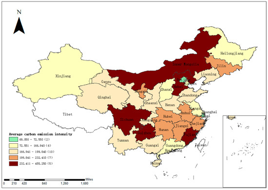
Figure 1.
Spatial distribution of the average CEICI (2010–2020).
The results reveal pronounced regional differences in the CEICI of China. In particular, the CEICI is found to be higher in western and central regions, which are regarded as less developed areas with a relatively low per capita GDP (data from the China Statistical Yearbook [65]), whereas the CEICI is found to be lower in well-developed eastern regions such as Beijing and Shanghai. As an exception, Fujian manifests a high level of CEICI, which can be attributed to the mounting carbon emissions arising from the expanding construction enterprises coupled with a subdued construction output in this area. Additionally, it is found that Hebei, Fujian, Sichuan, Guizhou, and Inner Mongolia exhibit a notably heightened CEICI, which aligns with the findings of related studies [73]. For example, Zhang et al. [7] noted an increased carbon emission intensity in western China.
3.2. The Static CEECI
3.2.1. Results of the CEECI
According to Formulas (9)–(10), Matlab was used to calculate the CEECI for each province in China with the super-efficient SBM model. Then, ArcGIS was further used to visually present the results of the CEECI, allowing for a detailed analysis of its spatial distribution characteristics. Due to technical limitations, it is not feasible to plot the CEECI bar charts for all years on a single map. Therefore, we have selected specific cross-sectional years, namely 2010, 2013, 2017, and 2020, for our analysis [39]. Figure 2 illustrates the average spatial distribution of the CEECI from 2010 to 2020, along with the bar chart depicting the CEECI for the years of 2010, 2013, 2017, and 2020.
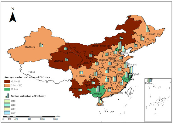
Figure 2.
The average spatial distribution of CEECI along with the bar chart of CEECI for the years of 2010, 2013, 2017, and 2020.
Figure 2 and the annual statistics (see Table A3 in Appendix A) reveal significant variations in the CEECI in China, with high levels mainly distributed in eastern and coastal areas and low levels mainly distributed in western areas. The average CEECI in Beijing (1.435), Shanghai (1.122), Zhejiang (1.028), and Guangxi (1.064) from 2010 to 2020 exceeded 1.0, indicating a higher level of carbon efficiency in comparison to other provinces in China. In contrast, provinces such as Inner Mongolia, Gansu, Qinghai, and Guizhou in the western region demonstrate low average annual efficiency levels of less than 0.5. The average annual CEECI in the western region of Inner Mongolia is 0.363, ranking the least among 30 provinces and cities in China.
3.2.2. Spatial Correlation Analysis
Moran’s I index is an important measure of spatial autocorrelation [74,75], which is divided into a global Moran’s I index and a local index. Specifically, the global Moran’s I index is used to detect the spatial pattern of the whole region, while the local index is used to reveal the heterogeneity of the local region [76]. To further analyze the spatial correlation in each province, GeoDa software was used to calculate the global Moran’s I of the CEECI from 2010 to 2020 based on the geographic distance spatial weight matrix, which is used to describe the average correlation degree observed in the whole region with the surrounding areas [77].
When −1 < Moran’s I < 0, the spatial correlation is negative. When 0 < Moran’s I < 1, the space is positively correlated. The calculation results are shown in Table 5.
Table 5.
Global Moran’s I for CEECI from 2010 to 2020.
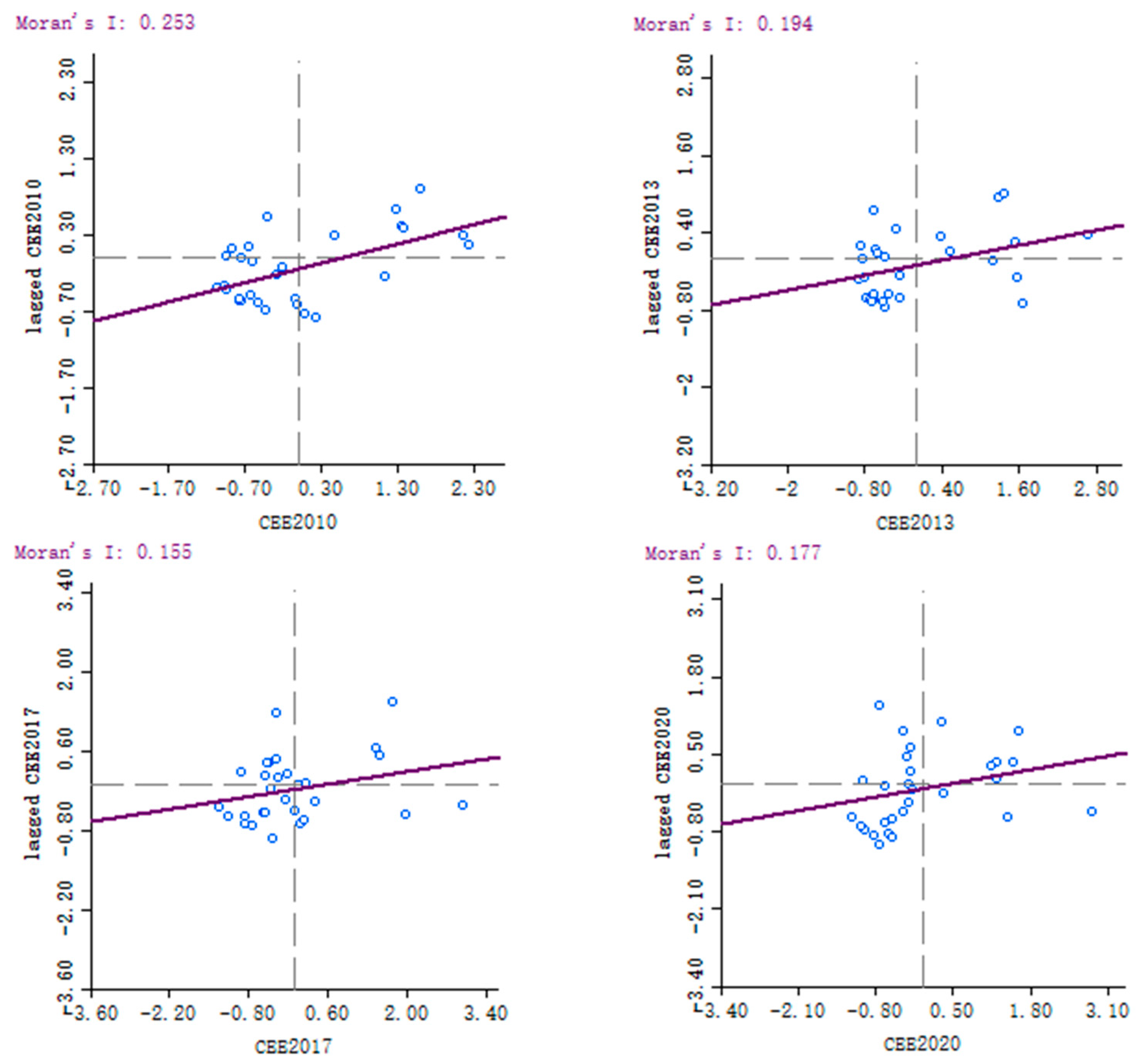
The results of the global Moran’s I reveal that every year, except for 2012, passed the significance test. The global Moran’s I of the CEECI is consistently greater than 0, indicating an obvious positive spatial autocorrelation. To further examine the correlation between the internal spatial units and the adjacent units, a local spatial correlation test was conducted. Due to space constraints, Figure 3 displays the Moran local scatter plots for the years 2010, 2013, 2017, and 2020.
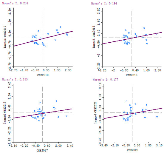
Figure 3.
Moran local scatter plot for 2010, 2013, 2017, and 2020.
Figure 3 illustrates that most provinces and cities are distributed in the first quadrant or the third quadrant, which indicates that there is a significant positive spatial correlation between the clustering of high CEECI areas and the clustering of low CEECI areas. The provinces and cities in the first quadrant are mostly located in the eastern region while those in the third quadrant are mostly located in the western region, indicating a mutual driving effect of the CEECI among the 30 provinces and cities. In general, the local distribution characteristics of the CEECI in each province exhibited relatively minor changes during 2010–2020. The number of provinces and cities in the first and third quadrants of the index remained relatively stable, and the overall spatial characteristics did not exhibit substantial changes between 2010 and 2020.
3.2.3. Results of the CRPCI
In accordance with Formulas (9) and (10), the relaxation variable Sz of carbon emissions was obtained, and the ratio of the relaxation variable (Sz) to the TCEs is the CRPCI [78,79,80]. The CRPCI represents the potential to reduce greenhouse gas emissions and achieve sustainable development goals through the implementation of emission reduction measures and technological innovations [81]. As the building industry is a significant contributor to carbon emissions, reducing its carbon footprint can lead to environmental improvements such as air quality enhancements, resource conservation, and economic benefits [82]. Therefore, quantifying the CEECI and evaluating the CRPCI can disclose the current challenges related to high carbon emissions and identify opportunities for improvement [83]. This assessment aids in the development and implementation of appropriate emission reduction measures, policies, and technological innovations, promoting the transition of the building industry to a low-carbon trajectory, reducing greenhouse gas emissions, and enhancing resource utilization efficiency. A larger CRPCI means that the region has excessive carbon emissions with more space for its reduction. The CRPCI of China was measured from 2010 to 2020, and the results are shown in Table 6.
Table 6.
The carbon emission reduction potential in the construction industry of 30 provinces and cities in China (2010–2020) (Unit: %).
This result shows the wide variation in the CRPCI values in different regions of China. It is worth noting that Inner Mongolia (68.43), Guizhou (62.13), Ningxia (55.80), Sichuan (53.04), and Hebei (53.02) have higher CRPCI values, with an average annual rate of more than 50%. On the other hand, the CRPCI value of Zhejiang, Beijing, and Shanghai is 0, which is significantly lower than other provinces and cities in China. In addition, the average annual CRPCI in Jiangsu is relatively small at less than 10%.
3.3. The Dynamic CEECI
By considering the static characteristics, the dynamic CEECI of 30 provinces and cities in China was further analyzed based on the ML index (see Table 7) obtained from Formula (11). The ML index of the construction industry in 30 provinces and cities in China is decomposed by Formulas (12)–(17). Table 8 presents the results for the years of 2010–2011, 2013–2014, 2016–2017, and 2019–2020.
Table 7.
ML index of the construction industry in 30 provinces and cities in China (2010–2020).
Table 8.
ML index decomposition of the construction industry in 30 provinces and cities in China for major years.
Overall, the ML index of most provinces and cities is greater than or close to 1, and the ML value of the eastern region is relatively lower than that of the central and western regions. According to the ML index decomposition model, the CEECI in the eastern region is affected by MLTC and MLPEC, while the increase of MLTC, MLPEC, and MLSEC in the western region is conducive to the increase of the CEECI, especially MLTC.
4. Discussion
4.1. Discussion and Analysis of TCEs
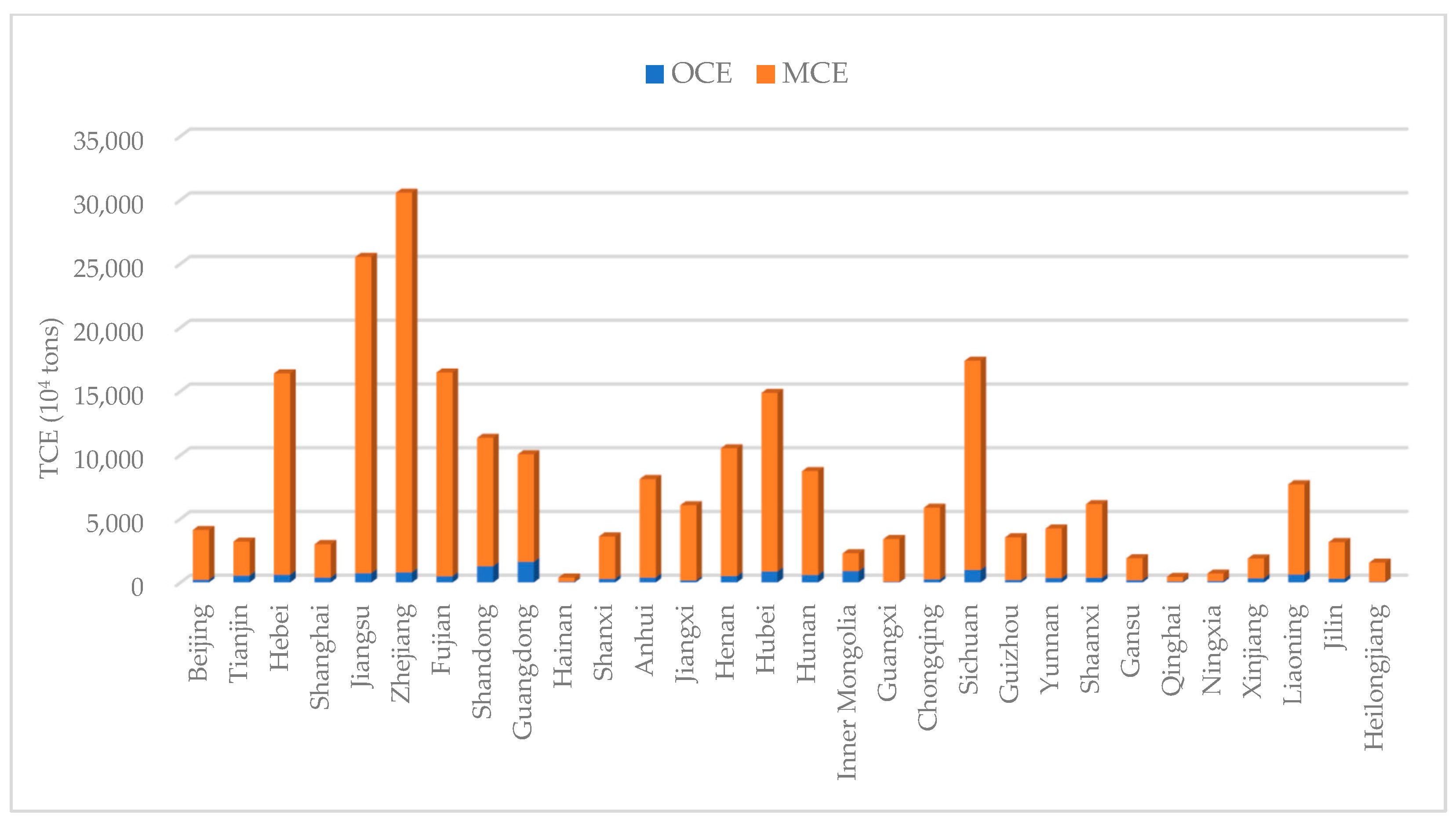
Due to limited studies attempting to achieve a systematic calculation of carbon emissions in various provinces in China, this study selected more comprehensive energy sources to achieve an accurate estimation of DCEs and employed the carbon emission coefficient method to measure ICE2. In order to further explore the results of the proportion of the OCEs and MCEs in the TCEs of Chinese provinces and cities, the average carbon emission and its composition histogram, as shown in Figure 4, were further analyzed.
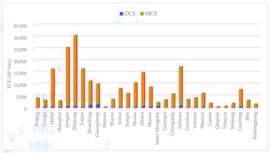
Figure 4.
The average of carbon emissions of 30 provinces and cities in China (2010–2020).
By comparing the collective share of the carbon emissions during the building operation stage (OCEs) and the share of the carbon emissions during the building materialization stage (MCEs) within the TCEs, it is found that the proportion of the MCEs is significantly higher than that of the OCEs in all provinces. The MCEs involve emissions generated from the construction stage, along with upstream industries (production and transportation of materials) and downstream industries (e.g., demolition). This is consistent with existing research findings [13,84]. For example, Du et al. [73] found that the MCEs accounted for about 90% of the TCEs. In addition, the prevalence of lower temperatures, extensive centralized heating areas, and the large proportion of heating energy within building operations contribute to a relatively elevated proportion of the OCEs in some specific northern provinces (e.g., Inner Mongolia, Tianjin, and Qinghai).
4.2. Discussion and Analysis of the Static CEECI
From the results of the CEECI and its spatial distribution map in Figure 2, it can be seen that the level of the CEECI in the eastern region is significantly higher than that in the central and western regions. This may be attributed to the heightened focus and strategic emphasis on the developed cities (Beijing, Shanghai, and Zhejiang) at the national level, along with a set of carbon emission reduction activities and a higher level of energy mix measures. Beijing, Shanghai, and Zhejiang are committed to promoting the development of clean energy, especially wind and solar energy, and increasing the proportion of renewable energy in their energy structures. In addition, the government has implemented incentive measures for green building projects to further promote carbon reduction activities [85]. The higher CEECI level in Guangxi Province is mainly attributed to its focus on green and energy-efficient building developments, resulting in significantly lower carbon emissions compared to other provinces and cities with similar building scales. For instance, Guangxi Province has issued the “Guangxi Green Building Action Plan” and established an energy-saving supervision system [86]. In addition, the relatively poor carbon emission efficiency of areas such as Inner Mongolia may be due to its unreasonable energy structure and the lack of technical personnel in the construction industry in the western areas. Mengna et al. [9] also found that the lower CEECI in Inner Mongolia was mainly attributed to conventional coal-dominated energy structures. This relationship underscores the positive correlation between regional economic developments and CEECI levels.
In general, the eastern region has a relatively open economy with a mature construction industry and a balanced allocation of production factors. Notably, a significant proportion of energy consumption in the eastern region comprises low carbon emission coefficient sources, such as natural gas and hydropower, contributing to the high level of CEECI in this area. On the contrary, the low level of CEECI in the western region can be attributed to its relatively less-advanced economic developments, which results in a less attractive environment for high-quality talents in the construction industry, leading to lower quality construction personnel and weaker technological advancements. Yang [27] also highlighted that although the CEECI is higher in the eastern region than in the western region, most provinces in China are experiencing a fluctuating upward trend. Du et al. [39] explained that the reasons for the lower CEECI levels in marginal cities (e.g., Xinjiang and Jilin) are the economic downturn, a continuous contraction of the construction market, and the lagging optimization of the energy structure, along with poor management practices in those areas.
4.3. Discussion and Analysis of the CRPCI
In order to better analyze and show the distribution of the CRPCI in different regions of China, the annual spatial distribution of the CRPCI was drawn, as shown in Figure 5.
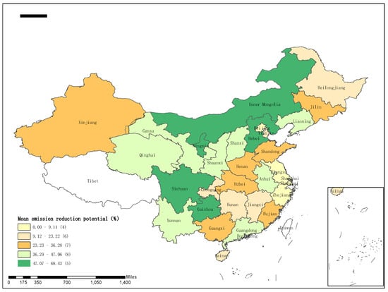
Figure 5.
Spatial distribution of the average CRPCI in China (2010–2020).
It can be seen from Figure 5 that the central and western regions demonstrate a higher CRPCI compared to the eastern region. Specific provinces and cities in eastern China, including Shanghai, Beijing, and Zhejiang, demonstrate zero potentials, indicating that they have already achieved an advanced level of CRPCI. In contrast, the central and western regions, such as Inner Mongolia, Guizhou, Ningxia, Sichuan, and Hebei, exhibit an average CRPCI exceeding 50%, highlighting a substantial scope for improvement in energy conservation and carbon emission reduction in these provinces. This finding is consistent with existing studies suggesting that there is great potential for emissions reduction in heating districts such as Inner Mongolia and Hebei [87]. Moreover, an examination of the CEECI reveals an inverse correlation with the CRPCI; that is, provinces and cities with a higher CRPCI tend to have a lower CEECI, whereas those with a lower potential exhibit a higher CEECI [88].
4.4. Discussion and Analysis of the Dynamic CEECI
Using the ML index model to study the dynamic CEECI, the ML index in the majority of the 30 provinces and cities is greater than or close to 1, suggesting a steady growth of the CEECI with a slowed-down growth rate in recent years. Some studies have also indicated that areas with a higher CEECI exhibit a relatively lower ML index and slower CEECI growth [89]. The eastern provinces generally have lower ML values with a slow growth rate, which may be due to the fact that they have achieved an excellent CEECI level [12]. Additionally, Beijing and Shanghai are exhibiting high values of ML while maintaining a high level of CEECI. This is mainly attributed to the advanced economic development of Beijing and Shanghai, which has driven local governments to allocate substantial funds for the adoption of low-energy and renewable building materials and to establish prominent standards and regulations for the green development of the construction sector [90,91]. For example, Beijing has issued a standard specification on the management of green building incentive funds [86], while Shanghai has mandated the adoption of assembly-type constructions for new civil and industrial buildings [92].
It can be concluded from Table 8 that the enhancement of the CEECI in all provinces and cities is mainly due to the impact of MLTC, which is consistent with existing studies [93,94]. From a regional perspective, the CEECI in the eastern region is affected by MLTC and MLPEC, and the decision-making unit is constantly moving to the production frontier and approaching the optimal scale. The construction industry in the eastern region has reached a certain scale, the economic development level is high, and the MLSEC has not significantly affected the improvement of the CEECI. The improvement of MLTC, MLPEC, and the MLSEC in the central and western regions is all conducive to promoting the improvement of the CEECI, indicating that these regions should pay particular attention to MLTC, accelerate the growth of low-carbon technologies, and improve the ML index. However, the ML index of the central and western regions as a whole shows a fluctuating upward trend, indicating that, with the continuous development of the construction industry in the central and western regions, it is approaching the optimal scale.
Despite the fact that this paper has conducted a relatively complete and systematic analysis of the CEECI of China, there are still some limitations in its calculation of MCEs and the scope of the analysis of the CEECI. First, the consumption data for building materials in China is primarily recorded in the China Statistical Yearbook on Construction [59], which only includes information on the consumption of steel, wood, cement, glass, and aluminum. Consequently, the calculated MCEs only take into account the carbon emissions generated by these five main building materials, potentially introducing a slight deviation into the calculation. Hence, it is recommended for researchers to further explore the impact of carbon emissions from building materials beyond these five main categories to determine the contribution of these additional materials to the total carbon emissions in the construction industry. This can provide a more comprehensive understanding of the carbon emissions profile of the sector. Second, conducting an analysis at the provincial level offers a macroscopic perspective but may overlook the subtle differences and variations within each province’s construction industry. Future research is recommended to focus on the municipal level within a province to investigate the variations of the CEECI among different cities. This can help evaluate the strengths and weaknesses of the emission reduction policies and measures implemented in these cities to complement the findings of the present study.
5. Conclusions and Policy Recommendations
This paper establishes a comprehensive carbon emission accounting model for the accurate measurement and analysis of carbon emissions in the construction industry in China. By employing the super-efficiency SBM model and the ML index model containing non-expected outputs, both the dynamic and static analyses of the CEECI in 30 provinces and cities were conducted. A spatial analysis of the CEECI and CRPCI was performed, which can provide valuable implications for policy designers to effectively mitigate carbon emissions. The main conclusions and policy recommendations are as follows:
(1) The TCEs of the Chinese construction industry shows a fluctuating upward trend, and the generated by the construction industry is the main component of the TCEs, indicating that the construction industry has a strong industry driving role. Consequently, the government should establish differentiated carbon emission reduction responsibility mechanisms for different industries and establish low-carbon management and implementation rules. For instance, the establishment of low-carbon awareness among different industries (e.g., steel and concrete) and the implementation of reward and penalty systems based on their levels of emissions can effectively mitigate the carbon emissions generated in the materialization stage.
(2) The CEECI varies significantly among provinces in China, and the CEECI in the eastern region is significantly higher than that in the central and western regions. The government should strengthen regional cooperation and mutually beneficial partnerships in order to overcome regional constraints and reduce disparities in the CEECI. Efforts should be made to facilitate the transfer of technology from the eastern regions to the central and western regions, with a particular focus on attracting skilled professionals in the construction industry. The positive role of high-efficiency areas in driving the development of low-efficiency areas should be fully utilized to achieve regionally coordinated developments. Additionally, since Beijing and Shanghai have the best CEECIs, their green building policies and regulations are advocated for adoption by other provinces and cities in China to facilitate green building developments nationwide.
(3) The CRPCI of China in different provinces varies significantly, and the CRPCI is found to be negatively correlated with the CEECI. The government should tailor economic and technological support based on the characteristics of each region, comprehensively taking local conditions into account. Provinces with a high CRPCI but a low CEECI should fully utilize the advantages of low-carbon policies and accelerate the development of clean technologies (e.g., renewable materials). Provinces with a high CRPCI should focus on optimizing industrial structures and resource allocations to further improve their CEECI. Taking inspiration from the clean energy initiatives promoted by Beijing, Shanghai, and Zhejiang, such as wind and solar power, efforts should be made to reduce reliance on traditional coal-dominated energy structures and to increase the proportion of renewable energy in the overall energy mix.
(4) From the dynamic decomposition results of the CEECI, MLTC is the main factor affecting the CEECI in each province and has a significant positive effect on the improvement of the CEECI. The government should increase scientific and technological investments and make overall plans. Technical issues such as heating and cooling efficiency and energy electrification should be prioritized. In addition, the construction industry in China’s provinces should strengthen technological transformations, such as replacing technical equipment that is not suitable for technical or economic use with new technical equipment.
Author Contributions
Conceptualization, J.Z. and M.C.; methodology, Y.Z.; software, Y.Z.; formal analysis, Y.Z.; investigation, Y.C.; resources, J.Z.; data curation, Y.Z.; writing—original draft preparation, Y.Z.; writing—review and editing, J.W. and M.C.; visualization, L.Z.; supervision, J.Z.; project administration, L.Z.; funding acquisition, J.Z. All authors have read and agreed to the published version of the manuscript.
Funding
This study was supported by the Practice and Innovation Fund for University Students of Jiangsu Province (202310304063Z).
Data Availability Statement
Not applicable.
Acknowledgments
This work was supported by the Practice and Innovation Fund for University Students of Jiangsu Province (202310304063Z). The authors thank all of the researchers who have been involved in this study: Jun Zhang, Ying Zhang, Yunjie Chen, Jinpeng Wang, Lilin Zhao, and Min Chen.
Conflicts of Interest
The authors declare no conflict of interest.
Appendix A
Table A1.
Carbon emissions of the construction industry from 2010 to 2020 (Unit: 104 tons).
Table A1.
Carbon emissions of the construction industry from 2010 to 2020 (Unit: 104 tons).
| Provinces | 2010 | 2011 | 2012 | 2013 | 2014 | 2015 | 2016 | 2017 | 2018 | 2019 | 2020 | Average |
|---|---|---|---|---|---|---|---|---|---|---|---|---|
| Beijing | 4141.10 | 4247.77 | 3435.60 | 3855.11 | 3991.27 | 3858.62 | 3655.28 | 3876.19 | 4616.35 | 4977.63 | 4636.69 | 4117.42 |
| Tianjin | 2180.10 | 2962.44 | 2921.30 | 3827.69 | 5124.88 | 3377.18 | 3066.20 | 2683.86 | 3917.30 | 2345.50 | 2887.00 | 3208.49 |
| Hebei | 11,931.56 | 50,978.83 | 50,098.14 | 18,619.91 | 8787.23 | 9145.52 | 6541.50 | 7026.63 | 5645.86 | 6563.21 | 5100.96 | 164,03.58 |
| Shanghai | 2683.57 | 2862.43 | 2711.69 | 2771.60 | 2850.15 | 2352.96 | 2424.72 | 2659.57 | 2582.21 | 5715.11 | 3413.71 | 3002.52 |
| Jiangsu | 17,446.34 | 29,870.23 | 32,186.46 | 24,667.14 | 26,506.67 | 24,510.53 | 24,102.46 | 24,053.74 | 25,803.79 | 24,940.07 | 26,773.66 | 25,532.83 |
| Zhejiang | 22,551.46 | 27,728.49 | 29,545.27 | 33,489.57 | 34,282.08 | 34,412.04 | 34,716.80 | 37,087.15 | 31,773.29 | 25,682.84 | 24,995.17 | 30,569.47 |
| Fujian | 6784.00 | 6664.42 | 8351.58 | 11,196.03 | 14,788.44 | 15,257.24 | 17,283.81 | 21,591.42 | 25,139.66 | 27,867.68 | 26,267.89 | 16,472.02 |
| Shandong | 9632.56 | 9778.67 | 22,368.62 | 10,686.56 | 11,149.21 | 10,562.08 | 9843.76 | 9792.52 | 10,052.95 | 11,333.09 | 9600.75 | 11,345.53 |
| Guangdong | 7009.04 | 10,127.94 | 10,306.67 | 9755.95 | 10,390.67 | 8726.73 | 8005.24 | 10,334.96 | 10,671.74 | 12,435.93 | 12,798.55 | 10,051.22 |
| Hainan | 268.49 | 430.32 | 415.05 | 515.16 | 405.61 | 266.53 | 302.59 | 331.99 | 454.03 | 465.23 | 393.19 | 386.20 |
| Shanxi | 4494.84 | 3095.55 | 3138.88 | 3297.47 | 3857.80 | 3518.09 | 3427.76 | 3630.51 | 3882.76 | 3787.12 | 3537.35 | 3606.19 |
| Anhui | 4519.68 | 4863.35 | 4905.01 | 6093.21 | 6607.09 | 5599.87 | 6943.01 | 8886.85 | 10,135.06 | 18,269.11 | 12,359.16 | 8107.40 |
| Jiangxi | 2285.25 | 3530.82 | 3801.32 | 4651.75 | 2297.18 | 6068.00 | 6466.47 | 8027.91 | 9170.38 | 10,437.02 | 9898.34 | 6057.68 |
| Henan | 7087.71 | 7281.73 | 8859.62 | 8525.09 | 11,723.72 | 8563.09 | 10,555.01 | 11,561.57 | 16,238.15 | 12,341.31 | 12,957.67 | 10,517.70 |
| Hubei | 4824.10 | 9355.86 | 16,766.38 | 15,564.60 | 18,350.34 | 14,754.54 | 19,784.64 | 17,360.74 | 17,852.62 | 14,421.98 | 14,508.45 | 14,867.66 |
| Hunan | 6142.03 | 6000.92 | 6912.98 | 7275.36 | 7619.36 | 7962.16 | 8714.58 | 9489.04 | 11,208.90 | 12,309.58 | 12,425.32 | 8732.75 |
| Inner Mongolia | 2063.54 | 2376.58 | 2290.73 | 2114.21 | 2085.44 | 2207.67 | 2553.85 | 3316.38 | 2515.35 | 1794.59 | 1811.30 | 2284.51 |
| Guangxi | 1907.17 | 2156.22 | 2940.48 | 3169.30 | 3533.47 | 3114.67 | 3957.46 | 4445.54 | 3766.46 | 4456.99 | 3960.43 | 3400.75 |
| Chongqing | 5007.53 | 5428.01 | 4810.03 | 5721.15 | 5850.80 | 5749.34 | 6325.33 | 6374.27 | 6328.41 | 6573.56 | 6385.13 | 5868.51 |
| Sichuan | 10,775.14 | 13,150.94 | 19,530.44 | 21,545.78 | 23,840.78 | 11,331.86 | 12,908.92 | 16,079.06 | 20,112.77 | 20,516.96 | 21,457.48 | 17,386.38 |
| Guizhou | 1040.72 | 1318.54 | 1624.78 | 2784.48 | 3403.56 | 4407.27 | 7880.68 | 3703.11 | 4292.21 | 4622.59 | 3836.98 | 3537.72 |
| Yunnan | 2347.06 | 2078.75 | 2576.87 | 5915.49 | 6472.38 | 3208.55 | 3807.53 | 4192.47 | 4956.26 | 5176.64 | 5747.87 | 4225.44 |
| Shaanxi | 3788.10 | 6280.58 | 4513.80 | 4821.53 | 5515.13 | 5627.84 | 6204.58 | 6354.95 | 7734.02 | 8005.90 | 8752.45 | 6145.35 |
| Gansu | 975.35 | 2122.99 | 1682.12 | 2090.38 | 2279.04 | 1988.81 | 2132.31 | 1862.40 | 1938.57 | 1647.23 | 2190.77 | 1900.91 |
| Qinghai | 573.40 | 330.01 | 346.55 | 366.79 | 396.53 | 391.06 | 416.94 | 507.48 | 519.98 | 463.93 | 503.29 | 437.81 |
| Ningxia | 506.34 | 646.52 | 633.60 | 821.17 | 953.18 | 702.07 | 628.94 | 626.39 | 693.35 | 909.82 | 558.23 | 698.15 |
| Xinjiang | 1144.42 | 1671.97 | 1927.40 | 2078.28 | 2602.63 | 1955.34 | 1928.41 | 1909.97 | 1693.89 | 1875.38 | 1910.06 | 1881.61 |
| Liaoning | 6602.81 | 10,681.55 | 9277.68 | 16,766.37 | 16,541.03 | 6068.53 | 5681.10 | 3467.76 | 3314.42 | 3084.19 | 3153.76 | 7694.47 |
| Jilin | 1741.40 | 2005.27 | 4815.41 | 7033.20 | 7466.20 | 2607.52 | 1857.23 | 1547.13 | 2251.32 | 2182.85 | 1243.56 | 3159.19 |
| Heilongjiang | 1432.66 | 2111.97 | 1653.23 | 1704.99 | 1736.29 | 1274.77 | 1270.41 | 1186.11 | 1199.92 | 2057.54 | 1428.20 | 1550.55 |
Table A2.
Total construction industry output of 30 provinces and cities in China from 2010 to 2020 (Unit: 108 RMB).
Table A2.
Total construction industry output of 30 provinces and cities in China from 2010 to 2020 (Unit: 108 RMB).
| Provinces | 2010 | 2011 | 2012 | 2013 | 2014 | 2015 | 2016 | 2017 | 2018 | 2019 | 2020 | Average |
|---|---|---|---|---|---|---|---|---|---|---|---|---|
| Beijing | 5196.02 | 6046.22 | 6588.30 | 7407.09 | 8209.80 | 8436.73 | 8841.19 | 9736.71 | 10,939.76 | 11,999.36 | 12,905.87 | 8755.18 |
| Tianjin | 2424.49 | 2986.45 | 3258.57 | 3670.53 | 4123.49 | 4488.90 | 4891.81 | 4262.35 | 3791.10 | 4096.50 | 4388.79 | 3853.00 |
| Hebei | 3231.46 | 3972.66 | 4865.09 | 5203.92 | 5625.75 | 5252.57 | 5517.69 | 5655.96 | 5740.25 | 5847.97 | 5948.09 | 5169.22 |
| Shanghai | 4300.19 | 4586.28 | 4843.44 | 5102.84 | 5499.94 | 5652.47 | 6046.19 | 6426.42 | 7072.21 | 7812.47 | 8277.04 | 5965.41 |
| Jiangsu | 12,405.92 | 15,122.85 | 18,423.55 | 21,712.16 | 24,592.93 | 24,785.81 | 25,791.76 | 27,956.71 | 30,846.66 | 33,099.18 | 35,251.64 | 24,544.47 |
| Zhejiang | 12,007.89 | 14,907.42 | 17,332.74 | 20,066.42 | 22,668.19 | 23,980.59 | 24,989.37 | 27,235.83 | 28,756.20 | 20,390.20 | 20,938.61 | 21,206.68 |
| Fujian | 2935.94 | 3692.62 | 4424.54 | 5459.41 | 6689.21 | 7605.81 | 8531.45 | 9993.65 | 11,548.82 | 13,164.42 | 14,118.01 | 8014.90 |
| Shandong | 5496.59 | 6482.90 | 7281.33 | 8332.70 | 9313.46 | 9381.72 | 10,087.43 | 11,477.75 | 12,898.29 | 14,269.29 | 14,947.30 | 9997.16 |
| Guangdong | 4715.46 | 5774.01 | 6514.43 | 7729.24 | 8356.50 | 8865.68 | 9652.31 | 11,372.05 | 13,714.37 | 16,633.41 | 18,429.84 | 10,159.75 |
| Hainan | 199.48 | 255.47 | 283.11 | 285.31 | 276.33 | 278.63 | 307.76 | 322.76 | 339.22 | 365.98 | 391.37 | 300.49 |
| Shanxi | 2143.46 | 2324.91 | 2668.17 | 2983.81 | 3103.49 | 2931.26 | 3318.47 | 3566.57 | 4071.46 | 4653.28 | 5113.64 | 3352.59 |
| Anhui | 2864.96 | 3597.26 | 4230.44 | 4970.34 | 5482.93 | 5695.94 | 6047.29 | 6829.67 | 7888.45 | 8503.26 | 9365.12 | 5952.33 |
| Jiangxi | 1690.02 | 2095.47 | 2789.57 | 3459.53 | 4122.63 | 4602.49 | 5179.03 | 6166.81 | 6993.40 | 7944.80 | 8649.16 | 4881.17 |
| Henan | 4400.61 | 5279.36 | 6009.08 | 7082.37 | 7911.89 | 8047.65 | 8807.99 | 10,086.58 | 11,360.52 | 12,701.68 | 13,122.56 | 8619.12 |
| Hubei | 4345.20 | 5586.45 | 7043.42 | 8343.40 | 10,059.59 | 10,592.86 | 11,862.40 | 13,390.73 | 15,133.87 | 16,979.67 | 16,136.11 | 10,861.24 |
| Hunan | 3161.73 | 3915.02 | 4407.92 | 5255.98 | 6020.97 | 6630.82 | 7304.22 | 8423.00 | 9581.44 | 10,800.62 | 11,864.03 | 7033.25 |
| Inner Mongolia | 1125.58 | 1394.68 | 1441.00 | 1540.48 | 1402.93 | 1123.47 | 1220.81 | 1122.19 | 1040.12 | 1086.06 | 1134.44 | 1239.25 |
| Guangxi | 1222.31 | 1553.07 | 1867.06 | 2271.39 | 2608.91 | 2953.42 | 3449.19 | 4210.07 | 4671.72 | 5407.31 | 5853.24 | 3278.88 |
| Chongqing | 2534.36 | 3328.83 | 3975.67 | 4731.88 | 5552.21 | 6256.94 | 7035.81 | 7605.66 | 7819.42 | 8222.96 | 8974.97 | 6003.52 |
| Sichuan | 4163.07 | 5256.65 | 6240.33 | 7239.49 | 8066.66 | 8768.24 | 9959.68 | 11,400.34 | 12,983.75 | 14,668.15 | 15,612.70 | 9487.19 |
| Guizhou | 622.96 | 824.72 | 1039.22 | 1365.00 | 1640.24 | 1947.74 | 2362.95 | 2932.96 | 3329.98 | 3714.89 | 4080.24 | 2169.17 |
| Yunnan | 1510.96 | 1868.40 | 2383.66 | 2888.82 | 3054.67 | 3268.93 | 3867.22 | 4726.36 | 5458.52 | 6122.09 | 6724.82 | 3806.77 |
| Shaanxi | 3063.61 | 3216.63 | 3529.39 | 3993.81 | 4557.71 | 4752.61 | 5329.23 | 6227.47 | 7120.15 | 7883.89 | 8501.13 | 5288.69 |
| Gansu | 751.99 | 925.84 | 1364.63 | 1708.27 | 1814.52 | 1849.02 | 1947.24 | 1825.42 | 1796.43 | 1916.35 | 2049.28 | 1631.73 |
| Qinghai | 279.61 | 319.42 | 325.76 | 396.39 | 432.91 | 409.51 | 410.62 | 406.93 | 435.14 | 460.72 | 512.24 | 399.02 |
| Ningxia | 342.69 | 427.92 | 466.95 | 564.66 | 625.16 | 524.53 | 511.25 | 549.21 | 565.04 | 601.41 | 641.81 | 529.15 |
| Xinjiang | 963.72 | 1320.37 | 1622.31 | 2071.52 | 2306.28 | 2255.74 | 2258.24 | 2418.70 | 2110.05 | 2278.17 | 2693.12 | 2027.11 |
| Liaoning | 4690.31 | 6217.52 | 7547.39 | 8743.37 | 7851.12 | 5413.76 | 3926.71 | 3688.33 | 3528.41 | 3554.45 | 3815.32 | 5361.52 |
| Jilin | 1348.78 | 1626.65 | 1990.43 | 2200.15 | 2521.00 | 2216.31 | 2283.56 | 2218.37 | 2183.63 | 1863.10 | 2005.78 | 2041.62 |
| Heilongjiang | 1769.70 | 2029.16 | 2373.96 | 2450.57 | 2150.75 | 1680.39 | 1716.61 | 1560.07 | 1194.28 | 1181.35 | 1206.37 | 1755.75 |
Table A3.
CEECI by provinces from 2010 to 2020.
Table A3.
CEECI by provinces from 2010 to 2020.
| Provinces | 2010 | 2011 | 2012 | 2013 | 2014 | 2015 | 2016 | 2017 | 2018 | 2019 | 2020 | Average |
|---|---|---|---|---|---|---|---|---|---|---|---|---|
| Beijing | 1.300 | 1.370 | 1.396 | 1.428 | 1.405 | 1.475 | 1.460 | 1.452 | 1.465 | 1.479 | 1.553 | 1.435 |
| Tianjin | 1.043 | 1.101 | 1.054 | 1.065 | 1.065 | 1.002 | 1.018 | 0.569 | 0.384 | 0.452 | 0.423 | 0.834 |
| Hebei | 0.446 | 0.451 | 0.415 | 0.505 | 0.676 | 0.540 | 0.593 | 0.540 | 0.538 | 0.623 | 0.599 | 0.539 |
| Shanghai | 1.125 | 1.114 | 1.033 | 1.036 | 1.038 | 1.126 | 1.138 | 1.120 | 1.180 | 1.267 | 1.165 | 1.122 |
| Jiangsu | 0.825 | 0.679 | 0.628 | 0.789 | 0.805 | 1.013 | 1.036 | 1.041 | 1.060 | 1.089 | 1.134 | 0.918 |
| Zhejiang | 1.064 | 1.097 | 1.089 | 1.111 | 1.117 | 1.086 | 1.086 | 1.058 | 1.105 | 0.739 | 0.751 | 1.028 |
| Fujian | 0.587 | 0.695 | 0.610 | 0.593 | 0.552 | 0.567 | 0.561 | 0.531 | 0.497 | 1.032 | 1.043 | 0.661 |
| Shandong | 0.408 | 0.455 | 0.359 | 0.447 | 0.524 | 0.552 | 0.556 | 0.571 | 0.601 | 0.650 | 0.589 | 0.519 |
| Guangdong | 0.467 | 0.520 | 0.414 | 0.492 | 0.523 | 0.552 | 0.554 | 0.525 | 0.488 | 0.656 | 0.548 | 0.522 |
| Hainan | 1.111 | 1.233 | 1.225 | 1.125 | 0.682 | 1.017 | 1.006 | 0.696 | 0.521 | 0.534 | 0.509 | 0.878 |
| Shanxi | 0.487 | 0.542 | 0.459 | 0.490 | 0.514 | 0.506 | 0.524 | 0.510 | 0.506 | 0.622 | 0.549 | 0.519 |
| Anhui | 0.522 | 0.605 | 0.497 | 0.501 | 0.545 | 0.685 | 0.630 | 0.568 | 0.535 | 0.512 | 0.585 | 0.562 |
| Jiangxi | 1.005 | 0.900 | 1.032 | 0.825 | 1.171 | 0.774 | 0.781 | 0.710 | 0.661 | 1.018 | 1.021 | 0.900 |
| Henan | 0.585 | 0.661 | 0.506 | 0.603 | 0.619 | 0.605 | 0.633 | 0.612 | 0.521 | 0.662 | 0.580 | 0.599 |
| Hubei | 0.533 | 0.585 | 0.464 | 0.538 | 0.620 | 0.647 | 0.707 | 0.675 | 1.048 | 1.064 | 1.048 | 0.721 |
| Hunan | 0.622 | 1.027 | 0.669 | 1.015 | 1.027 | 0.642 | 0.655 | 0.623 | 0.581 | 0.632 | 0.575 | 0.733 |
| Inner Mongolia | 0.495 | 0.500 | 0.421 | 0.428 | 0.380 | 0.334 | 0.332 | 0.294 | 0.243 | 0.290 | 0.278 | 0.363 |
| Guangxi | 0.719 | 1.012 | 1.020 | 1.121 | 1.141 | 1.099 | 1.152 | 1.180 | 1.040 | 1.110 | 1.108 | 1.064 |
| Chongqing | 0.690 | 0.690 | 0.590 | 0.605 | 0.759 | 0.848 | 0.830 | 0.754 | 0.750 | 0.783 | 0.762 | 0.733 |
| Sichuan | 0.494 | 0.545 | 0.468 | 0.493 | 0.502 | 0.595 | 0.562 | 0.506 | 0.482 | 0.583 | 0.490 | 0.520 |
| Guizhou | 0.438 | 0.534 | 0.458 | 0.431 | 0.458 | 0.422 | 0.354 | 0.403 | 0.354 | 0.367 | 0.336 | 0.414 |
| Yunnan | 0.490 | 0.576 | 0.423 | 0.442 | 0.437 | 0.530 | 0.513 | 0.517 | 0.488 | 0.571 | 0.456 | 0.495 |
| Shaanxi | 0.691 | 0.707 | 0.593 | 0.559 | 0.550 | 0.620 | 0.639 | 0.653 | 0.596 | 0.656 | 0.584 | 0.622 |
| Gansu | 0.447 | 0.470 | 0.442 | 0.477 | 0.486 | 0.569 | 0.546 | 0.454 | 0.392 | 0.383 | 0.328 | 0.454 |
| Qinghai | 0.527 | 0.575 | 0.396 | 0.460 | 0.463 | 0.468 | 0.390 | 0.338 | 0.316 | 0.367 | 0.347 | 0.422 |
| Ningxia | 0.557 | 0.615 | 0.535 | 0.533 | 0.540 | 0.484 | 0.464 | 0.420 | 0.424 | 0.449 | 0.471 | 0.499 |
| Xinjiang | 0.760 | 0.813 | 0.667 | 0.541 | 0.568 | 0.549 | 0.744 | 0.550 | 0.389 | 0.414 | 0.428 | 0.584 |
| Liaoning | 0.641 | 0.804 | 0.643 | 0.482 | 0.555 | 0.511 | 0.400 | 0.421 | 0.423 | 0.487 | 0.450 | 0.529 |
| Jilin | 1.067 | 1.013 | 0.433 | 0.540 | 1.019 | 0.593 | 0.673 | 0.681 | 0.523 | 0.451 | 0.493 | 0.681 |
| Heilongjiang | 1.277 | 1.122 | 1.187 | 1.147 | 1.110 | 1.007 | 1.011 | 0.702 | 0.436 | 0.406 | 0.394 | 0.891 |
References
- Du, M.B.; Zhang, X.L.; Xia, L.; Libin, C.; Zhe, Z.; Li, Z.; Heran, Z.; Cai, B.F. The China Carbon Watch (CCW) system: A rapid accounting of household carbon emissions in China at the provincial level. Renew. Sustain. Energy Rev. 2022, 155, 111825. [Google Scholar] [CrossRef]
- Liu, S.; Wang, Y.; Liu, X.; Yang, L.; Zhang, Y.; He, J. How does future climatic uncertainty affect multi-objective building energy retrofit decisions? Evidence from residential buildings in subtropical Hong Kong. Sustain. Cities Soc. 2023, 92, 104482. [Google Scholar] [CrossRef]
- Liu, X.; He, J.; Xiong, K.; Liu, S.; He, B.-J. Identification of factors affecting public willingness to pay for heat mitigation and adaptation: Evidence from Guangzhou, China. Urban Clim. 2023, 48, 101405. [Google Scholar] [CrossRef]
- Ma, C.B.; Atakelty, H.; You, C.Y. A critical review of distance function based economic research on China’s marginal abatement cost of carbon dioxide emissions. Energy Econ. 2019, 84, 104533. [Google Scholar] [CrossRef]
- The Catalyst Review Newsletter Group. Bp’s Statistical Review of World Energy 2021. Catal. Rev. Newsl. 2021, 34, 3. [Google Scholar]
- Jiao, J.L.; Yang, Y.F.; Bai, Y. The impact of inter-industry R&D technology spillover on carbon emission in China. Nat. Hazards 2018, 91, 913–929. [Google Scholar] [CrossRef]
- Zhang, X.; Fan, D. The Spatial-Temporal Evolution of China’s Carbon Emission Intensity and the Analysis of Regional Emission Reduction Potential under the Carbon Emissions Trading Mechanism. Sustainability 2022, 14, 7442. [Google Scholar] [CrossRef]
- Shen, L.; Song, X.; Wu, Y.; Liao, S.; Zhang, X. Interpretive Structural Modeling based factor analysis on the implementation of Emission Trading System in the Chinese building sector. J. Clean. Prod. 2016, 127, 214–227. [Google Scholar] [CrossRef]
- Zhang, M.N.; Li, L.S.; Cheng, Z.H. Research on carbon emission efficiency in the Chinese construction industry based on a three-stage DEA-Tobit model. Environ. Sci. Pollut. Res. 2021, 28, 51120–51136. [Google Scholar] [CrossRef]
- Ma, N.; Li, H.J.; Tang, R.W.; Dong, D.; Shi, J.L.; Wang, Z. Structural analysis of indirect carbon emissions embodied in intermediate input between Chinese sectors: A complex network approach. Environ. Sci. Pollut. Res. 2019, 26, 17591–17607. [Google Scholar] [CrossRef]
- Eggleston, H.S.; Buendia, L.; Miwa, K.; Ngara, T.; Tanabe, K. 2006 IPCC Guidelines for National Greenhouse Gas Inventories. 2006. Available online: https://www.osti.gov/etdeweb/biblio/20880391 (accessed on 20 March 2023).
- Zhou, W.Z.; Yu, W.H. Regional Variation in the Carbon Dioxide Emission Efficiency of Construction Industry in China: Based on the Three-Stage DEA Model. Discret. Dyn. Nat. Soc. 2021, 2021, 4021947. [Google Scholar] [CrossRef]
- Zhu, C.; Yang, Z.; Huang, B.; Li, X. Embodied Carbon Emissions in China’s Building Sector: Historical Track from 2005 to 2020. Buildings 2023, 13, 211. [Google Scholar] [CrossRef]
- Sun, Y.H.; Hao, S.Y.; Long, X.F. A study on the measurement and influencing factors of carbon emissions in China’s construction sector. Build. Environ. 2023, 229, 109912. [Google Scholar] [CrossRef]
- Nicholas, G.R.; Wassily, L.W. The Structure of the American economy, 1919–1939: An empirical application of equilibrium analysis. Econometrica 1951, 19, 351–353. [Google Scholar]
- Pan, W.; Pan, W.; Shi, Y.; Liu, S.; He, B.; Hu, C.; Tu, H.; Xiong, J.; Yu, D. China’s inter-regional carbon emissions: An in-put-output analysis under considering national economic strategy. J. Clean. Prod. 2018, 197, 794–803. [Google Scholar] [CrossRef]
- Long, Y.; Yoshida, Y.; Fang, K.; Zhang, H.; Dhondt, M. City-level household carbon footprint from purchaser point of view by a modified input-output model. Appl. Energy 2019, 236, 379–387. [Google Scholar] [CrossRef]
- Acquaye, A.A.; Duffy, A.P. Input–output analysis of Irish construction sector greenhouse gas emissions. Build. Environ. 2009, 45, 784–791. [Google Scholar] [CrossRef]
- Feng, B.; Wang, X.; Liu, B. Provincial Variation in Energy Efficiency Across China’s Construction Industry with Carbon Emission Considered. Resour. Sci. 2014, 36, 1256–1266. [Google Scholar]
- Li, Y.; Wang, J.F.; Liu, B.; Li, H.Y.; Guo, Y.M.; Guo, X.R. Regional green total factor performance analysis of China’s construction industry based on a unified framework combining static and dynamic indexes. Environ. Sci. Pollut. Res. 2022, 30, 26874–26888. [Google Scholar] [CrossRef]
- Solow, R.M. Technical change and the aggregate production function. Rev. Econ. Stat. 1957, 39, 554–562. [Google Scholar] [CrossRef]
- Hu, J.-L.; Wang, S.-C. Total-factor energy efficiency of regions in China. Energy Policy 2006, 34, 3206–3217. [Google Scholar] [CrossRef]
- Cheng, Z.; Li, L.; Liu, J.; Zhang, H. Total-factor carbon emission efficiency of China’s provincial industrial sector and its dynamic evolution. Renew. Sustain. Energy Rev. 2018, 94, 330–339. [Google Scholar] [CrossRef]
- Yang, Z.; Ying, K.; Tuo, Z. The spatial and temporal evolution of provincial eco-efficiency in China based on SBM modified three-stage data envelopment analysis. Environ. Sci. Pollut. Res. 2020, 27, 8557–8569. [Google Scholar]
- Sun, W.; Huang, C.C. Predictions of carbon emission intensity based on factor analysis and an improved extreme learning machine from the perspective of carbon emission efficiency. J. Clean. Prod. 2022, 338, 130414. [Google Scholar] [CrossRef]
- Zhang, C.Q.; Chen, P.Y. Industrialization, urbanization, and carbon emission efficiency of Yangtze River Economic Belt-empirical analysis based on stochastic frontier model. Environ. Sci. Pollut. Res. 2021, 28, 66914–66929. [Google Scholar] [CrossRef]
- Yang, Z.; Fang, H.; Xue, X.S. Sustainable efficiency and CO2 reduction potential of China’s construction industry: Application of a three-stage virtual frontier SBM-DEA model. J. Asian Arch. Build. Eng. 2022, 21, 604–617. [Google Scholar] [CrossRef]
- Anze, Z.; Yuan, Q. Research on Energy Efficiency Evaluation and Emission Reduction Strategy of Construction Industry Based on DEA and Improved FAA. IOP Conf. Ser. Earth Environ. Sci. 2018, 199, 022065. [Google Scholar] [CrossRef]
- Yao, X.; Feng, W.; Zhang, X.; Wang, W.; Zhang, C.; You, S. Measurement and decomposition of industrial green total factor water efficiency in China. J. Clean. Prod. 2018, 198, 1144–1156. [Google Scholar] [CrossRef]
- Yu, Y.G.; Yan, Y.N.; Shen, P.Y.; Li, Y.T.; Ni, T.H. Green financing efficiency and influencing factors of Chinese listed construction companies against the background of carbon neutralization: A study based on Three-Stage DEA and system GMM. Axioms 2022, 11, 467. [Google Scholar] [CrossRef]
- Sun, C.; Yan, X.; Zhao, L. Coupling efficiency measurement and spatial correlation characteristic of water–energy–food nexus in China. Resour. Conserv. Recycl. 2021, 164, 105151. [Google Scholar] [CrossRef]
- Thompson, M.; Dahab, M.F.; Williams, R.E.; Dvorak, B. Improving energy efficiency of small water-resource recovery facilities: Opportunities and barriers. J. Environ. Eng. 2021, 146, 05020005. [Google Scholar] [CrossRef]
- Zhou, Z.B.; Li, K.; Liu, Q.; Tao, Z.; Lin, L. Carbon footprint and eco-efficiency of China’s regional construction industry: A life cycle perspective. J. Oper. Res. Soc. 2021, 72, 2704–2719. [Google Scholar] [CrossRef]
- Yang, W.; Li, L. Analysis of Total Factor Efficiency of Water Resource and Energy in China: A Study Based on DEA-SBM Model. Sustainability 2017, 9, 1316. [Google Scholar] [CrossRef]
- Tone, K. A slacks-based measure of efficiency in data envelopment analysis. Eur. J. Oper. Res. 2001, 130, 498–509. [Google Scholar] [CrossRef]
- Zhang, Y.; Xu, X.Y. Carbon emission efficiency measurement and influencing factor analysis of nine provinces in the Yellow River basin: Based on SBM-DDF model and Tobit-CCD model. Environ. Sci. Pollut. Res. 2022, 29, 33263–33280. [Google Scholar] [CrossRef]
- Hua, L.; Min, Z. Carbon emission efficiency of construction industry in Hunan province and measures of carbon emission reduction. Nat. Environ. Pollut. Technol. 2019, 18, 1005–1010. [Google Scholar]
- Song, M.L.; Chen, Y.; An, Q.X. Spatial econometric analysis of factors influencing regional energy efficiency in China. Environ. Sci. Pollut. Res. 2018, 25, 13745–13759. [Google Scholar] [CrossRef]
- Du, Q.; Deng, Y.G.; Zhou, J.; Wu, J.; Pang, Q.Y. Spatial spillover effect of carbon emission efficiency in the construction industry of China. Environ. Sci. Pollut. Res. 2021, 29, 2466–2479. [Google Scholar] [CrossRef]
- Zhou, Y.X.; Liu, W.L.; Lv, X.Y.; Chen, X.H.; Shen, M.H. Investigating interior driving factors and cross-industrial linkages of carbon emission efficiency in China’s construction industry: Based on Super-SBM DEA and GVAR model. J. Clean. Prod. 2019, 241, 118322. [Google Scholar] [CrossRef]
- Jiang, X.H.; Ma, J.X.; Zhu, H.Z.; Guo, L.C.; Huang, Z.G. Evaluating the Carbon Emissions Efficiency of the Logistics Industry Based on a Super-SBM Model and the Malmquist Index from a Strong Transportation Strategy Perspective in China. Int. J. Environ. Res. Public Health 2020, 17, 8459. [Google Scholar] [CrossRef]
- Tian, J.J.; Song, X.Q.; Zhang, J.S. Spatial-Temporal Pattern and Driving Factors of Carbon Efficiency in China: Evidence from Panel Data of Urban Governance. Energies 2022, 15, 2536. [Google Scholar] [CrossRef]
- Xu, G.; Zhao, T.; Wang, R. Research on Carbon Emission Efficiency Measurement and Regional Difference Evaluation of China’s Regional Transportation Industry. Energies 2022, 15, 6502. [Google Scholar] [CrossRef]
- Zhou, Y.W. Total factor productivity of Hubei transportation industry under environmental constraint. Ekoloji Dergisi. 2019, 107, 1591–1597. [Google Scholar]
- Zhang, N.; Zhou, P.; Kung, C. Total-factor carbon emission performance of the Chinese transportation industry: A boot-strapped non-radial Malmquist index analysis. Renew. Sustain. Energy Rev. 2015, 41, 584–593. [Google Scholar] [CrossRef]
- Lin, B.; Fei, R. Regional differences of CO2 emissions performance in China’s agricultural sector: A Malmquist index approach. Eur. J. Agron. 2015, 70, 33–40. [Google Scholar] [CrossRef]
- Liu, M.; Yang, L. Spatial pattern of China’s agricultural carbon emission performance. Ecol. Indic. 2021, 133, 108345. [Google Scholar] [CrossRef]
- Zhang, X.; Liao, K.; Zhou, X. Analysis of regional differences and dynamic mechanisms of agricultural carbon emission efficiency in China’s seven agricultural regions. Environ. Sci. Pollut. Res. 2022, 29, 38258–38284. [Google Scholar] [CrossRef]
- Yao, X.; Guo, C.; Shao, S.; Jiang, Z. Total-factor CO2 emission performance of China’s provincial industrial sector: A meta-frontier non-radial Malmquist index approach. Appl. Energy 2016, 184, 1142–1153. [Google Scholar] [CrossRef]
- Oathout, J.M. Determining the Dynamic Efficiency with which wiping Materials Remove Liquids from Surfaces. Int. Nonwovens J. 2000, OS-9(1). [Google Scholar] [CrossRef]
- Lu, X.; Xu, C. The difference and convergence of total factor productivity of inter-provincial water resources in China based on three- stage DEA-Malmquist index model. Sustain. Comput. Inform. Syst. 2019, 22, 75–83. [Google Scholar] [CrossRef]
- Woo, C.; Chung, Y.; Chun, D.; Seo, H.; Hong, S. The static and dynamic environmental efficiency of renewable energy: A Malmquist index analysis of OECD countries. Renew. Sustain. Energy Rev. 2015, 47, 367–376. [Google Scholar] [CrossRef]
- Zhang, Z.; Liu, R. Carbon emissions in the construction sector based on input-output analyses. J. Tsinghua Univ. (Sci. Technol.) 2013, 53, 53–57. [Google Scholar]
- State Statistical Bureau (SSB; Now NBS). China Energy Statistical Yearbook; China Statistics Press: Beijing, China, 2022. Available online: http://www.shujuku.org/china-energy-statistical-yearbook.html (accessed on 20 November 2022).
- State Administration for Market Regulation. General Rules for Calculation of the Comprehensive Energy Consumption; National Standard of the People’s Republic of China, 2020. Available online: http://ft.panzhihua.gov.cn/uploadfiles/202108/12/2021081217202347802674.pdf (accessed on 20 January 2023).
- National Development and Reform Commission. Guidelines for the Preparation of Provincial Greenhouse Gas Inventories (Trial); National Development and Reform Commission: Beijing, China, 2011.
- Ministry of Ecology and Environment. Accounting Methods and Reporting Guidelines for Greenhouse Gas Emissions of Enterprises; China Energy Information Platform, 2015. Available online: http://big5.mee.gov.cn/gate/big5/www.mee.gov.cn/xxgk2018/xxgk/xxgk06/202212/W020221221671986519778.pdf (accessed on 20 December 2022).
- Construction Statistics National Bureau of Statistics. China Statistical Yearbook on Construction; China Statistics Press: Beijing, China, 2022; Available online: http://www.shujuku.org/china-construction-statistical-yearbook.html (accessed on 20 January 2023).
- Cui, P.; Li, D.; Ang, S.; Li, Q. Study on the life-cycle eco-efficiency evaluation method of residential building. Constr. Econ. 2013, 11, 96–99. [Google Scholar]
- Li, Z. Study on calculation method of life cycle energy consumption for recyclable materials. J. Basic Sci. Eng. 2006, 1, 50–58. [Google Scholar]
- Wang, L. Re-discussing CO2 reduction in China’s cement industry. China Cem. 2008, 2, 36–39. [Google Scholar]
- Li, X.; Xu, H. Life cycle evaluation of steel based on GaBi software. Environ. Prot. Circ. Econ. 2009, 29, 15–18. [Google Scholar]
- Lin, B.Q. Qualitative Change of China’s Energy Conservation and Emission Reduction Policy: From Energy Intensity to Carbon Intensity. China Daily. 2009. Available online: http://www.chinadaily.com.cn/zgrbjx/2009-11/05/content_9089221.htm (accessed on 20 February 2023).
- Fang, L.; Lu, T.; Kai, C.; Li, J.; Ping, S. Spatial distribution and regional difference of carbon emissions efficiency of industrial energy in China. Sci. Rep. 2021, 11, 19419. [Google Scholar]
- National Bureau of Statistics (NBS; formerly State Statistical Bureau). China Statistical Yearbook; China Statistics Press: Beijing, China, 2022. Available online: http://www.stats.gov.cn/sj/ndsj/ (accessed on 20 January 2023).
- Cheng, G. Data Envelopment Analysis Methodology and MaxDEA Software; Intellectual Property Publishing House: Beijing, China, 2014. [Google Scholar]
- Sten, M. Index numbers and indifference surfaces. Trab. Estad. 1953, 4, 209–242. [Google Scholar]
- Färe, R.; Margaritis, S.; Margaritis, D. Malmquist productivity indexes and DEA. In Handbook on Data Envelopment Analysis; Springer: Berlin/Heidelberg, Germany, 2011; pp. 127–149. [Google Scholar]
- Zhang, C.; Liu, H.; Bressers, H.T.A.; Buchanan, K.S. Productivity growth and environmental regulations—Accounting for undesirable outputs: Analysis of China’s thirty provincial regions using the Malmquist–Luenberger index. Ecol. Econ. 2011, 70, 2369–2379. [Google Scholar] [CrossRef]
- Du, J.; Chen, Y.; Huang, Y. A Modified Malmquist-Luenberger Productivity Index: Assessing Environmental Productivity Performance in China. Eur. J. Oper. Res. 2018, 269, 171–187. [Google Scholar] [CrossRef]
- Chung, Y.H.; Färe, R.; Grosskopf, S. Productivity and Undesirable Outputs: A Directional Distance Function Approach. J. Environ. Manag. 1997, 51, 229–240. [Google Scholar] [CrossRef]
- Du, Q.; Zhou, J.; Pan, T.; Sun, Q.; Wu, M. Relationship of carbon emissions and economic growth in China’s construction industry. J. Clean. Prod. 2019, 220, 99–109. [Google Scholar] [CrossRef]
- Du, Q.; Lu, X.; Yi, L.; Min, W.; Li, B.; Ming, Y. Carbon emissions in China’s construction industry: Calculations, factors and regions. Int. J. Environ. Res. Public Health 2018, 15, 1220. [Google Scholar] [CrossRef] [PubMed]
- Li, W.; Sun, W.; Li, G.; Cui, P.; Wu, W.; Jin, B. Temporal and spatial heterogeneity of carbon intensity in China’s construction industry. Resour. Conserv. Recycl. 2017, 126, 162–173. [Google Scholar] [CrossRef]
- Monidipa, D.; Ghosh, S.K. Measuring Moran’s I in a cost-efficient manner to describe a land-cover change pattern in large-scale remote sensing imagery. IEEE J.-Stars. 2017, 10, 2631–2639. [Google Scholar]
- Chen, H.; Lu, X.; Gao, T.; Chang, Y. Identifying hot-spots of metal contamination in campus dust of Xi’an, China. Int. J. Environ. Res. Public Health 2016, 13, 555. [Google Scholar] [CrossRef] [PubMed]
- Tang, Y.C.; Xia, N.N.; Varga, L.; Tan, Y.T.; Hua, X.J.; Li, Q.M. Sustainable international competitiveness of regional construction industry: Spatiotemporal evolution and influential factor analysis in China. J. Clean. Prod. 2022, 337, 130592. [Google Scholar] [CrossRef]
- Du, K.; Lu, H.; Yu, K. Sources of the potential CO2 emission reduction in China: A nonparametric metafrontier approach. Appl. Energy 2014, 115, 491–501. [Google Scholar] [CrossRef]
- Lu, C.-C.; Chiu, Y.-H.; Shyu, M.-K.; Lee, J.-H. Measuring CO2 emission efficiency in OECD countries: Application of the Hybrid Efficiency model. Econ. Model. 2013, 32, 130–135. [Google Scholar] [CrossRef]
- Wang, K.; Wei, Y.-M. China’s regional industrial energy efficiency and carbon emissions abatement costs. Appl. Energy 2014, 130, 617–631. [Google Scholar] [CrossRef]
- Tan, X.; Lai, H.; Gu, B.; Zeng, Y.; Li, H. Carbon emission and abatement potential outlook in China’s building sector through 2050. Energy Policy 2018, 118, 429–439. [Google Scholar] [CrossRef]
- Hou, H.; Feng, X.; Zhang, Y.; Bai, H.; Ji, Y.; Xu, H. Energy-related carbon emissions mitigation potential for the construction sector in China. Environ. Impact Assess. Rev. 2021, 89, 106599. [Google Scholar] [CrossRef]
- Guo, X.; Zhu, L.; Fan, Y.; Xie, B. Evaluation of potential reductions in carbon emissions in Chinese provinces based on en-vironmental DEA. Energy Policy 2011, 39, 2352–2360. [Google Scholar] [CrossRef]
- Zhang, Z.; Wang, B. Research on the life-cycle CO2 emission of China’s construction sector. Energy Build. 2016, 112, 244–255. [Google Scholar] [CrossRef]
- Beijing Municipal Commission of Housing and Urban-rural Development; Beijing Municipal Commission of Planning and Natural Resources; Beijing Municipal Finance Bureau. Beijing prefabricated buildings, green buildings, green ecological demonstration zone project municipal incentive funds management Interim measures. Gaz. People’s Gov. Beijing Munic. 2020, 38, 11–23. [Google Scholar]
- Development and Reform Commission, Department of Housing and Urban-Rural Development. Guangxi: Issued a green building action plan. Informatiz. China Constr. 2013, 22, 6. [Google Scholar]
- Xiao, H.; Wei, Q.; Wang, H. Marginal abatement cost and carbon reduction potential outlook of key energy efficiency technologies in China’s building sector to 2030. Energy Policy 2014, 69, 92–105. [Google Scholar] [CrossRef]
- Bian, Y.; Lv, K.; Yu, A. China’s regional energy and carbon dioxide emissions efficiency evaluation with the presence of recovery energy: An interval slacks-based measure approach. Ann. Oper. Res. 2015, 255, 301–321. [Google Scholar] [CrossRef]
- Zhang, J.; Zeng, W.; Wang, J.; Yang, F.; Jiang, H. Regional low-carbon economy efficiency in China: Analysis based on the Super-SBM model with CO2 emissions. J. Clean. Prod. 2017, 163, 202–211. [Google Scholar] [CrossRef]
- GB/T 50378-2019; Assessment Standard for Green Building. National Standard of the People’s Republic of China: Beijing, China, 2019.
- Report on Building Energy Efficiency and Green Building Policy and Development of Shanghai. Shanghai Build. Mater. 2014, 4, 1–6.
- Shanghai Housing and urban and rural Construction Management Committee requires that new civil and industrial buildings should be fabricated. Build. Technol. Dev. 2019, 46, 143.
- Cheng, Z.; Li, L.; Liu, J. Industrial structure, technical progress and carbon intensity in China’s provinces. Renew. Sustain. Energy Rev. 2018, 81, 2935–2946. [Google Scholar] [CrossRef]
- Yan, D.; Lei, Y.; Li, L.; Song, W. Carbon emission efficiency and spatial clustering analyses in China’s thermal power industry: Evidence from the provincial level. J. Clean. Prod. 2017, 156, 518–527. [Google Scholar] [CrossRef]


Disclaimer/Publisher’s Note: The statements, opinions and data contained in all publications are solely those of the individual author(s) and contributor(s) and not of MDPI and/or the editor(s). MDPI and/or the editor(s) disclaim responsibility for any injury to people or property resulting from any ideas, methods, instructions or products referred to in the content. |
© 2023 by the authors. Licensee MDPI, Basel, Switzerland. This article is an open access article distributed under the terms and conditions of the Creative Commons Attribution (CC BY) license (https://creativecommons.org/licenses/by/4.0/).