Abstract
The refurbishment of a social interest building using Earth-to-Air Heat Exchanger (EAHE) was studied in representative dry climatic conditions of Mexico (dry, very dry, temperate, and sub-temperate). A simulation method that uses both computational fluid dynamics (CFD) and building energy simulation (BES) was used to analyze the influence of the EAHE on the indoor conditions of a room. First, CFD simulations of the EAHE were performed using climatic data and soil properties of the four representative cities, and then the results were loaded into the TRNSYS software to estimate the indoor air temperature and the building room’s thermal loads. When connected to a building room on a warm day, the EAHE reduced the indoor air temperature by a factor ranging between 1.7 and 3.2 °C, while on a cold day, the EAHE increased the indoor air temperature of the room by between 1.0 and 1.9 °C. On the other hand, the EAHE reduced the daily cooling load of the room by a factor between 2% and 6%. The EAHE also reduced the daily heating load by between 0.3% and 11%. Thus, EAHE as a refurbishment technology can benefit social interest buildings in Mexico.
1. Introduction
Currently, daily human life is very attached to technology. For instance, we use air conditioning systems to achieve thermal comfort. This technology allows activities to be carried out more comfortably, especially in zones with extreme weather conditions. However, air conditioners are large electricity consumers; thus, energy refurbishment technologies currently seek to condition indoor spaces with the lowest possible energy consumption. One of these refurbishment alternatives is the Earth-to-Air Heat Exchanger (EAHE), which supplies airflow to the indoor environment of buildings [1,2,3]. This airflow improves indoor air conditions without consuming a high amount of electricity because of the use of the thermal inertia of the soil. In an EAHE, the ambient air is supplied by a fan to one or more pipes buried in the soil at a depth where the outdoor environment has a small influence. Because the soil temperature is different from the ambient temperature, the airflow in the pipes exchanges heat with the soil, which acts as a heat source or sink depending on the season or climatic zone [4]. Thus, the air from the buried pipes is cooled or heated and sent to the buildings to benefit their indoor thermal comfort. The amount of heat exchanged between the air in the pipe and the soil depends on various factors such as weather conditions, pipe length, diameter, and soil properties. Several researchers have studied the EAHE by performing experimental tests. Those studies have provided information about the effectiveness of EAHE in reducing or increasing airflow temperature. The capacity of EAHE to cool or heat the air depends on its design and the thermophysical properties of the soil. The following points can be highlighted regarding the design of EAHE:
- An EAHE installed in soil with a high humidity level presents better thermal performance and better air temperature drops than EAHE installed in dry soil [5,6].
- An airspeed between 1 and 5 m/s provides good airflow at the EAHE outlet; however, this reduces the time of interaction between the ground and the air, reducing the temperature difference between the inlet and the outlet [7].
- There are no significant changes in results concerning the material of the pipes [8].
- The temperature of the soil surrounding the pipe increases as time passes, which can be between 6 and 12 h of continuous operation of the system, and this increase in temperature decreases the capacity of the EAHE to reduce the temperature of the air at the outlet [9,10,11].
- A diameter between 25 and 30 cm reduces pressure drops in the pipe [12].
- The drop or rise in temperature to the air caused by the EAHE can reach values between 2 and 20 °C and the cooling or heating capacity ranges between 2000 and 8000 W. Those values vary depending on weather conditions, construction parameters, and soil type [13,14,15,16,17,18,19,20].
The previous findings have allowed a better understanding of how an EAHE behaves; however, studying an EAHE by performing experimental tests requires considerable time and might be expensive. Thus, EAHE has also been studied theoretically to subject it to different conditions and understand the influence of various parameters on its thermal behavior. Many of these studies have certain similarities in developing their mathematical models, such as the following: constant soil and air thermophysical properties, constant air velocity, and laminar, transitional, or turbulent flow. These models are usually solved using computational fluid dynamics (CFD) [21]. On the other hand, most analytical studies consider one-dimensional models, generally whose formulations are solved using the thermal resistance method. Another notable difference is that the analytical studies consider steady-state conditions, while most numerical studies consider EAHE in an unsteady state [22]. These differences make analytical studies easier to develop but limited in representing reality, while numerical studies have higher accuracy but are relatively complex. Other computational tools, such as TRNSYS, implement components (type 952 and 997) where, by means of finite differences, they model the heat conduction between the pipe and the surrounding soil.
Some works have analyzed the influence of the soil temperature on the behavior of EAHE [12,23,24,25,26,27]. Other studies have considered different passive systems coupled to the EAHE [28,29,30,31,32]. Some studied different EAHE configurations [2,33,34,35] or different weather and soil conditions in which the EAHE interacts [36]. The results of these studies have allowed us to understand which soil conditions benefit the EAHE. For instance, a high humidity level in the soil or soil moisture benefits the thermal potential of the EAHE [37,38]. The typical configuration of an EAHE is a horizontal pipe. However, for its optimal operation, long lengths are sometimes needed, so various designs can allow long lines in a reduced space, such as the spiral configuration, serpentine, and others known as Z because of the way the fluid travels [39,40,41,42,43]. In the case of climatic conditions, the system works better for extreme weather conditions and deficient ambient humidity levels compared to mild and humid climates [34,44,45].
Other research works have mentioned that the EAHE can increase the ventilation potential of buildings. Thus, some researchers have evaluated the EAHE system connected to a room. Maytorena and Hinojosa [46] numerically analyzed the thermal behavior of an EAHE connected to a building room in the dry zone of Sonora, Mexico. The research was divided into four cases, where the authors determined the temperature inside the room while thermally insulating some walls and allowing heat gain in others. They showed that the EAHE maintained the indoor air between 27 and 29 °C regardless of where the heat gain was activated. Other authors, such as Ahmed et al. [15], experimentally studied the conditioning capacity of the EAHE connected to a room in a warm humid zone in Rockhampton, Australia. The authors found that the EAHE reduced the indoor air temperature by 2.1 °C, while the humidity level increased by 1.2%. Other works such as Skotnicka-Siepsiak [47] have studied the energy capacity of the EAHE connected to a room in Olsztyn, Poland. The results showed that the system reduced 45% of the energy consumption of the room by providing 75% of the cooling energy required by the room. Other studies were conducted to analyze different passive systems coupled to a room. For instance, Long et al. [48] studied the benefits of connecting a solar chimney with phase change material (PCM) with an EAHE. The results showed that the airflow of the EAHE increases by 50% when coupling this system to a solar chimney with PCM and with 0.8 °C lower indoor room temperature than the case without PCM.
An EAHE may have excellent cooling or heating potential, which is defined as the air temperature difference between the outlet and the inlet. Still, when the supply airflow to the room is insufficient, it could not benefit the indoor environment regardless of the supply air temperature. Previous works of the authors of the current research have numerically analyzed the performance of an EAHE for different cities in Mexico [49,50,51]. Although those studies showed that the EAHE had an acceptable thermal performance for most climatic zones, they do not reveal how the airflow from the EAHE could benefit the indoor environment of a building. Therefore, this work aims to estimate the influence of an EAHE on the indoor air temperatures and heating and cooling loads of a room that belongs to a social interest building situated in regions representing the different dry climate conditions of Mexico. For this purpose, a coupling was carried out between computational fluid dynamics (CFD) and TRNSYS (BES). First, a CFD model was used to perform simulations of the EAHE in four cities, and then the results were loaded into the TRNSYS V16 software through a data reader to estimate a building room’s cooling and heating loads.
2. Physical Model
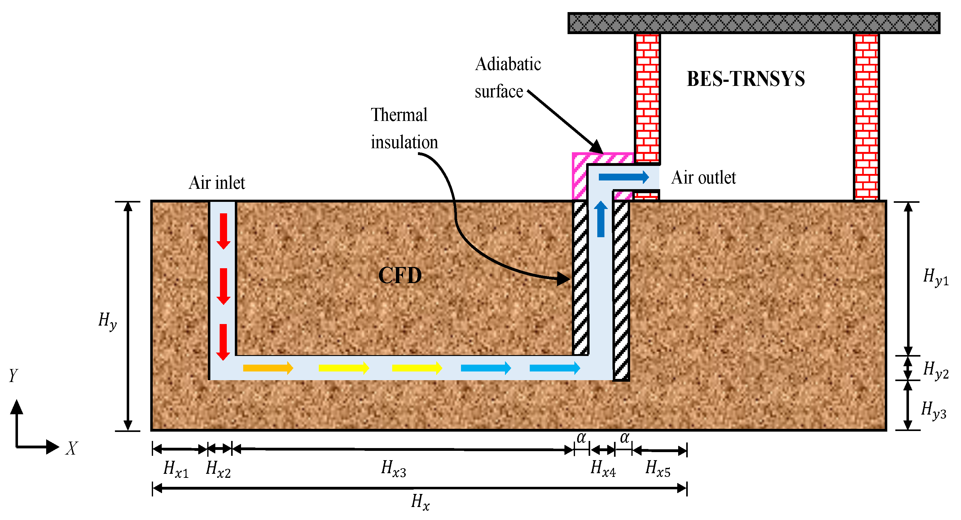
The EAHE was modeled with a typical horizontal configuration. The system consists of a 5 m long PVC D30 pipe buried at 2 m. The dimensions of the EAHE are due to the space available in low-income housing, whose dimensions are between 30 and 50 m. A 0.05 m insulation layer was considered to minimize energy losses or gains in the vertical outlet pipe of the EAHE. It is supposed that the air that is introduced to the building room has the same temperature and velocity as the air at the outlet of the EAHE. Thus, it is assumed that the elbow that connects the EAHE with the room is adiabatic and does not interrupt the airflow or cause additional head losses. Figure 1 shows the geometry of the EAHE, while its dimensions are shown in Table 1.

Figure 1.
Physical model of the Earth-to-Air Heat Exchanger (EAHE) connected to a room.

Table 1.
Dimensions of the different sections of the EAHE.
The assumptions for numerical modeling are shown in Figure 2. For the soil section (Figure 2a), we assume the following:
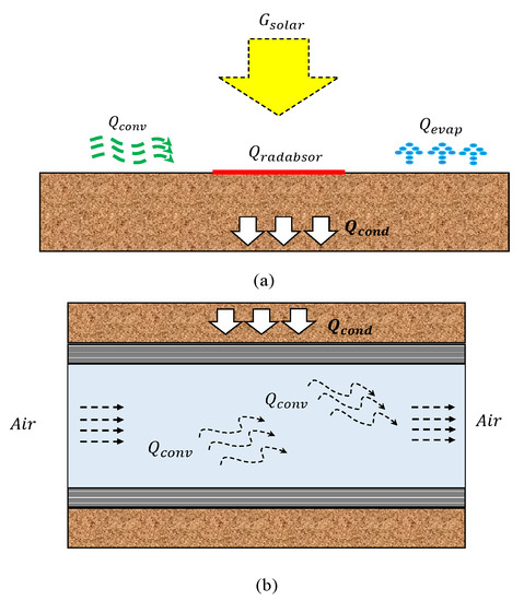
Figure 2.
Heat transfer processes: (a) soil and (b) interior of the pipe.
- Two-dimensional heat transfer.
- Constant and temperature-independent thermophysical properties of soil.
- The temperature of the soil is determined by solving the heat conduction equation affected by the boundary conditions of the surface exposed to the outdoor environment.
For the pipe (Figure 2b), we assume the following:
- The pipe of the circular cross-section is modeled as a square cross-section of equivalent area [52].
- The heat conduction of the pipe wall is not considered because the thickness is very thin.
- There is no evaporation or condensation in the pipes of the EAHE.
- Convection heat transfer is the dominant mechanism in the pipes.
- There is laminar and transitional airflow inside the pipes because it is considered that a low-power fan will supply the air.
Room
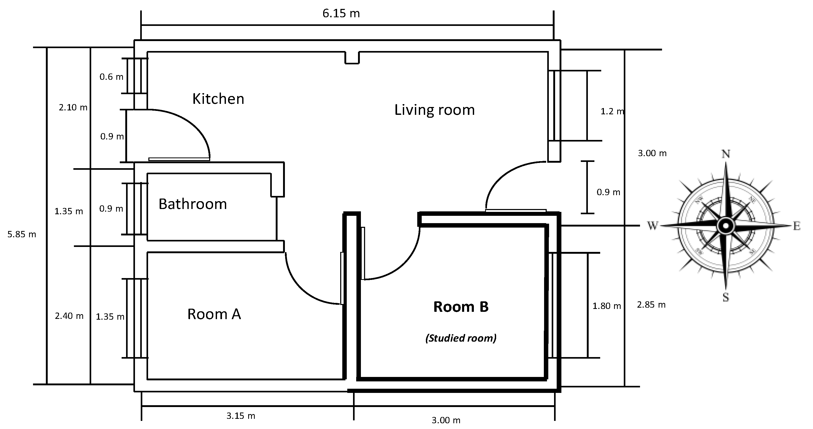
In Mexico, homes are classified according to their surface area and price, with the residential plus being the largest and most expensive, and those with the lowest price and size are called social interest. The latter is between 30 and 50 m in size [53], and consists of two bedrooms, a living–dining room, a kitchen, and a bathroom, as shown in Figure 3.

Figure 3.
Plant view of the social interest building.
The room selected for the coupling of the system is the largest bedroom of the building from Figure 3 (room B), with dimensions of 3 × 2.85 m. The room is highlighted in the Figure and the orientation of the building is also shown. The room’s height was established according to the housing building code, which specifies that it must be 2.7 m [53].
Table 2 shows the thermophysical properties of the construction materials of the analyzed building used in the simulation together with the thicknesses of each one, whose values were obtained from the TRNSYS materials library. These materials were used to form the walls, roof, and floor configuration, which were defined as a composition of one or several layers of material, from the inside to the outside; the building envelope components are composed as follows:
Table 2.
Thermophysical properties of the materials of the building room.
- Exterior walls (exposed to outdoor environment): a layer of gypsum plaster, a layer of mortar, brick, and a layer of mortar.
- Interior walls (exposed to indoor environment): a layer of mortar, brick, and a layer of mortar.
- Floor: a layer of marble, lime cement mortar, and a layer of light concrete.
- Roof: a layer of gypsum plaster, a layer of mortar, hollow block, lime cement mortar, and a waterproofing layer.
3. Mathematical Model of the EAHE
The system analyzed is formed by the soil and EAHE. The mathematical model considers the heat conduction in the soil and heat transfer by convection in laminar and transitional regime inside the pipes. The governing equations of the heat transfer phenomenon are continuity, momentum, and energy, which are discretized using the finite volume method. These equations can be solved in a transient state; however, it requires a lot of resources and computational time. Thus, the quasi-transient state was used, which consists of modeling steady states every ten minutes. The governing equations are as follows:
The system is subject to four boundary conditions, three adiabatic and one in which an energy balance occurs, proposed by Mihalakakou et al. [22]; these conditions are detailed below.
- (a)
- Left and right boundaries (x = 0, ) are considered adiabatic:
For the bottom boundary, the current work uses the concept of penetration depth used by some research works available in the literature [54,55]. This concept assumes that the daily heat wave (the daily oscillation in temperature of the outdoor air entering the EAHE) does not penetrate the soil beyond a certain radius, and this radius is lower than 1 m in the y downward direction. Therefore, this boundary can be considered as an adiabatic boundary after a certain depth. The bottom boundary can be expressed as follows:
- (b)
- Bottom boundary (y = 0):
- (c)
- Upper boundary (). To represent the heat transfer in the northern boundary on the soil surface, the following energy balance proposed by Mihalakauko et al. [22] was used:
- (i)
- CE is the convective energy exchanged between the air and the soil surface:is the temperature of the environment according to the day, and is the temperature of the soil surface. is the convection heat transfer coefficient on the soil surface and it is determined from the following equations [56]:
- (ii)
- is the short wavelength solar radiation absorbed from the soil surface, which is calculated by Mihalakauko et al. [22]:is the absorptance of the soil and G is the solar radiation that reaches the surface of the soil.
- (iii)
- is the long wavelength radiation, which can be calculated as follows:is the emittance of the soil surface and is a term that depends on the relative humidity of the earth and air at the surface. A value of 63 W/m has proven to be a good approximate value for this variable, shown in Badescu [56].
- (iv)
- is the latent heat flux from the soil surface due to evaporation, which can be calculated as follows [22]:is the relative humidity of the ambient air and f is a number that is a function of the type of land cover. This fraction can take the following values:
- (d)
- Supplied airflow (). It is considered that the temperature of air entering the pipes is equal to the temperature of the outdoor environment at a constant velocity, which is governed by the Reynolds number value.
- (e)
- Outgoing air flow ().
For the numerical solution of the EAHE model, the governing equations of the system (soil + pipe thermal insulation + air) were solved as if it all was fluid, and the thermophysical properties were assigned according to the position in the system. In the solid region (soil and pipe thermal insulation), a blocking-off method was used, which consists of setting up the velocity components equal to zero. In this way, the hydrodynamic effect in the soil and insulation is canceled, and heat transfer is then governed only by heat conduction. In the fluid region (inside the pipes), such a blocking-off method was not used; therefore, the velocity and temperature fields were obtained for this region. In the current research, the soil temperature was not considered to be equal to the annual average outdoor air temperature, as the bottom boundary condition of the model. Instead, the soil temperature is determined by solving the mathematical model and its boundary conditions. The solution provides the temperature distribution of the soil, which depends on the type of soil, the upper boundary condition, which is affected by the outdoor environment, and the interaction with the pipes of the EAHE.
Numerical Modeling of the EAHE
The finite volume technique divides the physical domain into small control volumes. In this work, the finite volume technique uses a Cartesian grid and does not specify a z direction. Heat transfer in the z direction is considered negligible. A computational node is placed where the desired variable is calculated in each volume. Interpolation schemes were implemented to discretize the governing equations, using the central scheme for the conductive terms and a hybrid scheme for the convective ones. The SIMPLE algorithm was implemented for coupling the momentum and continuity equations [57,58]. A convergence criterion of 10 was established for all variables to ensure good results and precision.
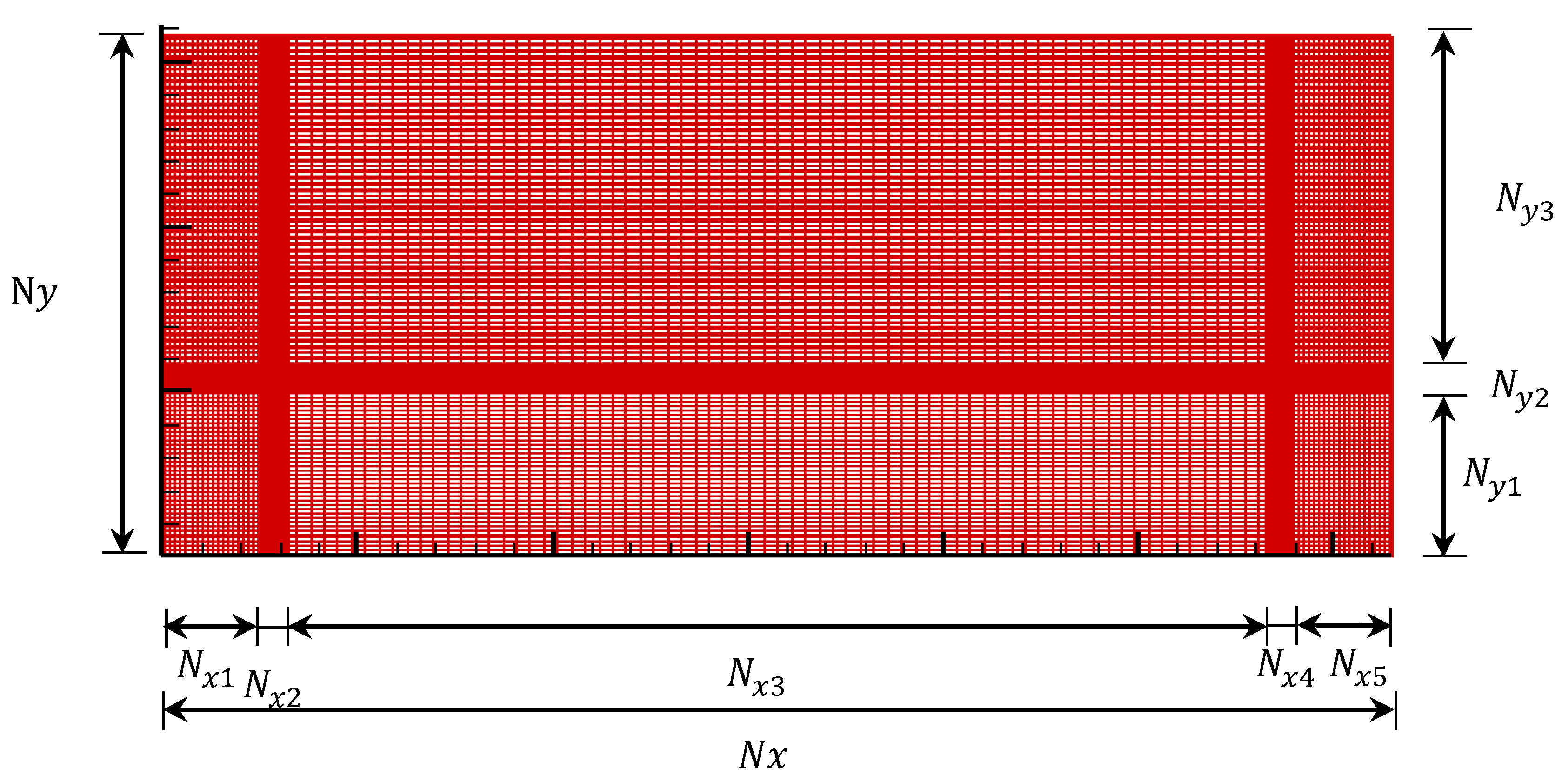
The optimal number of control volumes into which the domain can be divided varies in each case study. Thus, it is necessary to carry out a mesh independence study to find the number of volumes that allow the best precision in the results without consuming extra computational resources. Figure 4 shows the division of the physical domain in a computational mesh. The spaces separating the pipe volumes are more refined than those corresponding to the soil. The meteorological conditions for the mesh independence study were those of Juárez City because it is the place with the most extreme climate. The temperature was 46.6 °C with solar radiation of 786 W/m, and the relative humidity was 5% with a wind speed of 1.5 m/s.
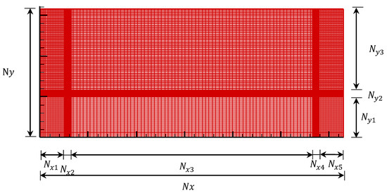
Figure 4.
Computational domain of the EAHE.
The mesh independence study consisted of varying the number of nodes representing the pipe length () from 71 to 111 nodes, while the rest of the sections remained constant. The results showed that after 101 nodes, there are no significant changes in the velocity and temperature of the air in the outlet. Once the number of nodes was established for the length of the pipe, the number of nodes varied in the sections of , , and from 50 to 90 nodes. From 71 nodes, it was observed that the outlet air temperature and speed no longer varied significantly. The number of nodes in the physical domain is 286 in the x-direction and 215 in the y-direction; the distribution is presented in Table 3.
Table 3.
Number of nodes used for each section of EAHE.
The computational code was verified by solving the exercise available in House et al. [59]. The exercise determines the velocities and temperatures of the air laminar flow regime in steady state by natural convection in a cavity with an embedded solid in the center. The cavity has a vertical hot wall ( = 25 °C) and a vertical cold wall ( = 15 °C). The dimension of cavity H is determined based on the Rayleigh number for conductivity ratios of 0.2 and 0.5 in which the Nusselt number was compared. The verification results showed that the absolute percentage difference between the results of this study and results obtained by House et al. [59] is 0.6% and 0.7% for the conductivity ratios mentioned above. Thus, the developed computational code provides reliable results. Other verification tests performed for the computational code used here can be found in previous publications of the authors of the current work [50,60].
4. BES-CFD Coupling
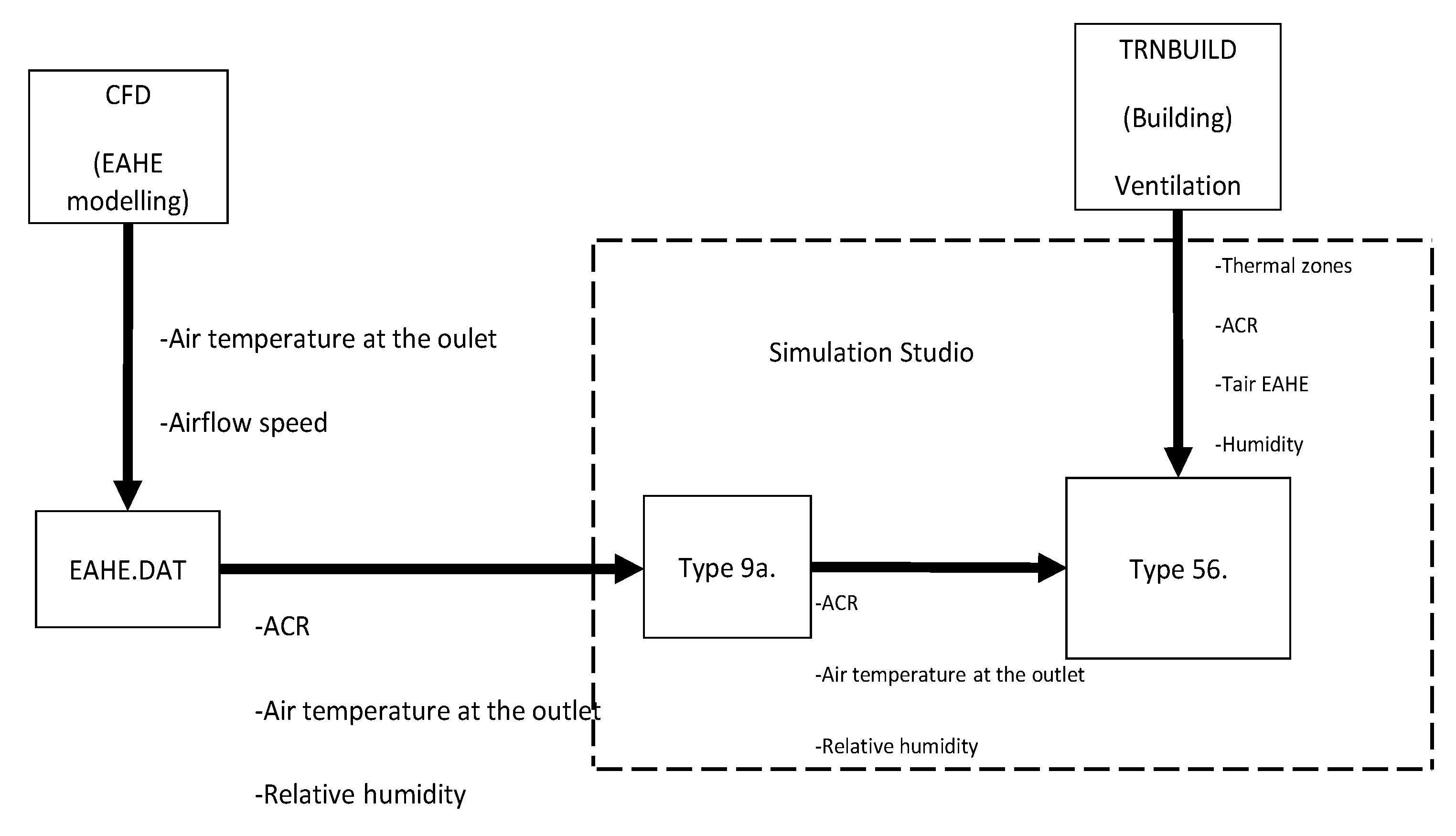
The BES-CFD coupling is a technique that allows us to take advantage of both parties in heat transfer analysis. The BES-CFD coupling can be of a dynamic type when both programs work together, exchanging information at each moment, or static when the programs work using the information received from the other, but they work independently. These benefits include reduced time and computational resources of convergence in CFD, more exact heat transfer coefficients used in BES, and better estimation of building energy requirements compared to standalone BES simulations [61]. In this study, a static coupling was implemented where the TRNSYS building modeling software implements the data obtained from the CFD numerical modeling through the following procedure:
- From the numerical modeling of EAHE, a .txt file is obtained, which contains the air temperature at the outlet of the EAHE, the air changes per hour, and the air humidity of each modeled case.
- The VENTILATION component is activated in the TRNbuild interface, and the variables are named.
- The .txt file is read through a data reader in the simulation studio, which supplies the TYPE 56 component with the variables required by the VENTILATION component.
The BES-CFD coupling is carried out using a data reader and TYPE 56, as shown in Figure 5.

Figure 5.
Diagram of the static coupling.
The room simulation in TRNSYS was carried out under free-floating conditions to analyze the influence of the EAHE on thermal comfort. The thermal loads for each chosen city’s warmest and coldest days were also calculated to explore the effect of the EAHE on the thermal loads.
5. Climatic Conditions and Soil Properties
For the numerical modeling or CFD simulations, the ambient temperature, wind speed, and relative humidity of warmest and coldest days of four representative cities with dry climate present in Mexico were used as input data in 10 min intervals. These cities were selected based on their prevailing climate. The climatic data were provided by the National Meteorologic Service—National Commission of Water (SMN-CONAGUA). However, it is not possible to show all of the input data used in simulations, so here are presented only the average, maximum, and minimum values of the climatic data used in simulations (Table 4). These data were obtained from the warmest and coldest days of the year 2020. The same climatic data used for the CFD simulations were used to perform the simulations of the social interest building using TRNSYS.
Table 4.
Summary of the climatic conditions of the four analyzed cities.
To perform the CFD simulations it is also necessary to have the properties of the soil in each of the representative cities in Mexico. Thus, according to previous research [62,63], the types of soil in each city are Mexico City (silt), Juarez City (sand), Zacualtipan (limestone rock), and Monterrey (limestone rock). Table 5 presents the thermophysical properties of the different types of soil considered in the current work.
Table 5.
Thermophysical properties of different types of soil [51].
6. Results
This section is divided into two parts. The first part presents the running schedule of the EAHE, which is determined by comparing the temperature of the air at the outlet of the EAHE and the temperature of the indoor air in the room. The second part presents the influence of connecting an EAHE on the indoor air temperatures and cooling and heating loads of the building room.
6.1. Determination of the EAHE Running Schedule
The numerical modeling of the heat exchanger was carried out for different air velocities, according to the Reynolds number in laminar and transitional flow. This section compares the temperature of the indoor air in the room, determined with TRNSYS, and the temperature of air supplied by the EAHE in each city, which was obtained with CFD simulation. This comparison allowed us to discriminate which schedule the EAHE works well with and which it does not. Therefore, if the EAHE does not comply with its duty of cooling or heating as needed, it is supposed that the air from EAHE does not enter the room.
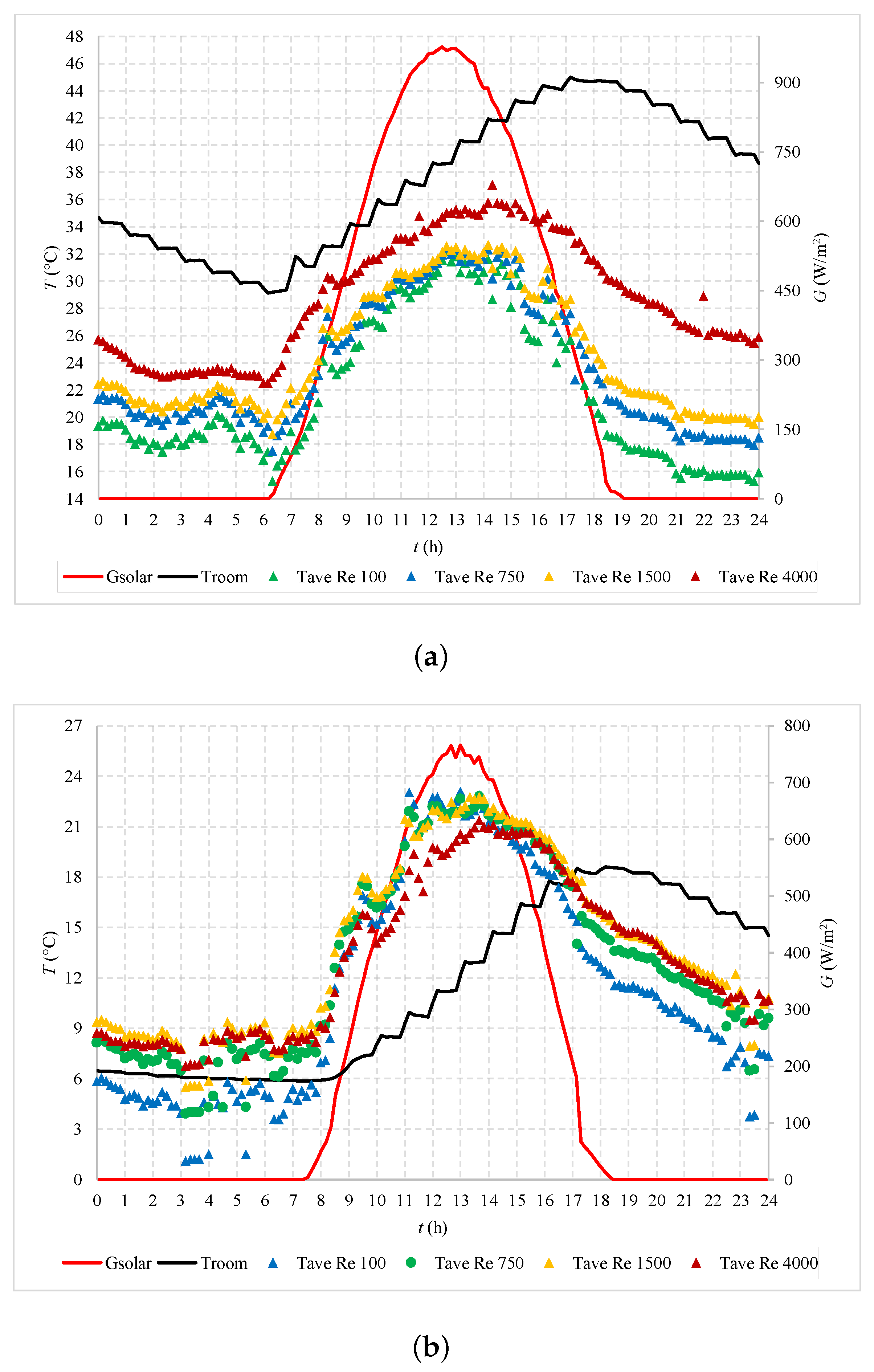
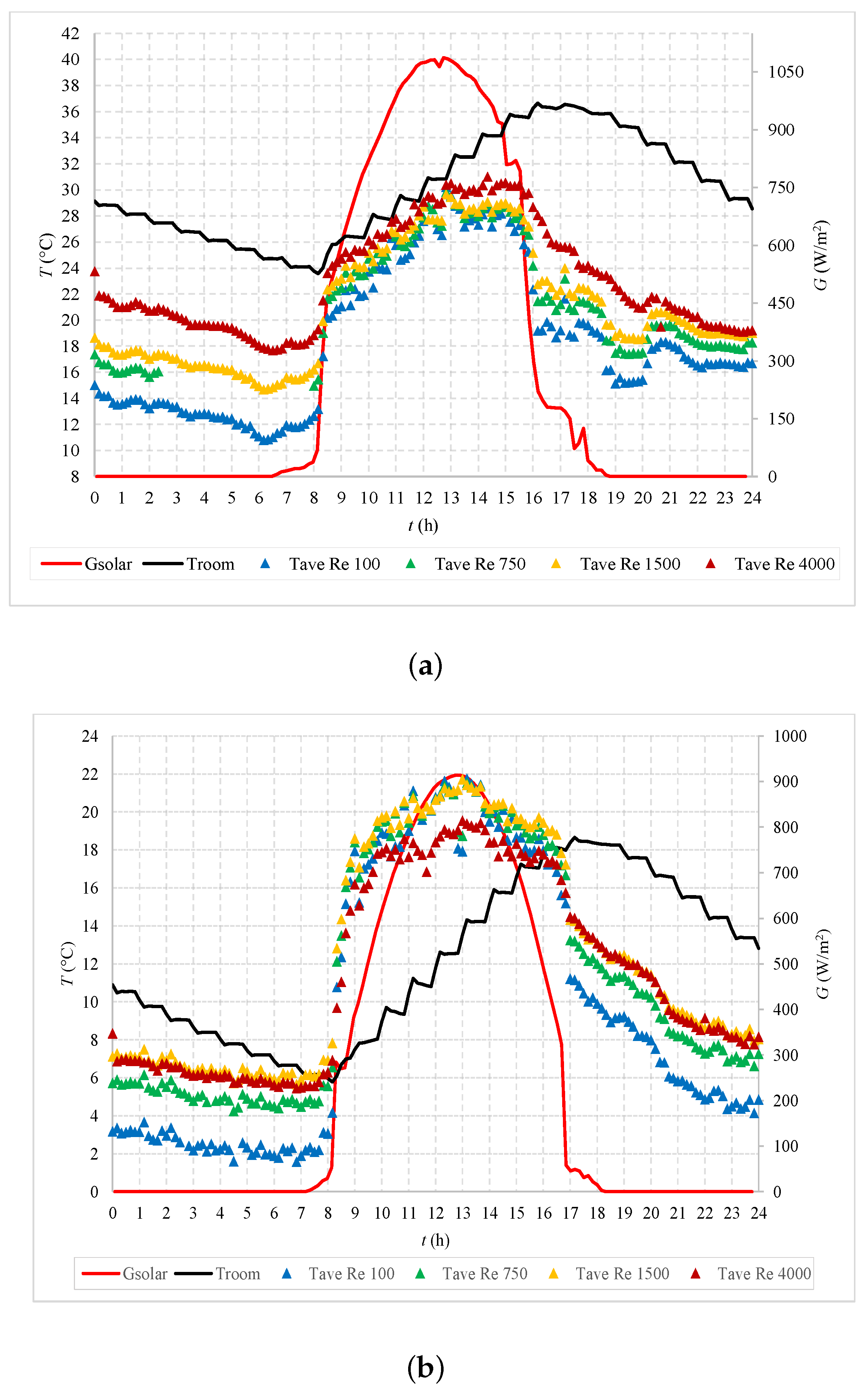
Figure 6a shows a graphical comparison between the indoor air temperature of the room without EAHE and the air temperature at the outlet of the EAHE on the warmest day in Monterrey. Different air velocities for the air into the pipes are presented in the figure as a function of the Reynolds number (). On this day, the indoor air temperature of the building room ranges between 29.5 and 45 °C. The air from the EAHE is colder than the indoor air of the room the whole day for any value of . During the first seven hours, between 00:00 h and 07:00 h, the air from the EAHE was up to 15 °C colder than the indoor air. This temperature difference tends to decrease as solar radiation increases; however, it remains below room temperature, with a difference of 7 °C between 7:00 and 13:00 h for small Reynolds values. When the radiation decreases, around 16:00 h, the air temperature from the outlet of the EAHE decreases.
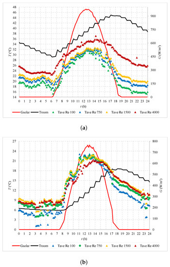
Figure 6.
Comparison between the temperature of the air supplied by the EAHE and the indoor air of the room in Monterrey: (a) warmest day and (b) coldest day.
On the coldest day in Monterrey, the air temperature supplied by the EAHE and the indoor air temperature in the room are shown in Figure 6b. The indoor air temperature of the building room ranges between 6 and 18.6 °C. Thus, the room in this city requires heating to reach thermal comfort, especially the period before 14:00 h. Figure 6b shows that the airflow provided by the EAHE is warmer than the air in the room during most of the day at high . As solar radiation increases, this heating effect tends to be greater from 08:00 h, with a temperature difference of about 11 °C. However, as solar radiation decreases, the EAHE loses the heating effect. The supplied air temperature becomes lower than that of the room from 16:00 h, with a temperature difference of about 11 °C. This behavior makes it unfeasible to keep the system running when the room reaches a temperature close to 15 °C; thus, the EAHE could only provide 17 h of heating.
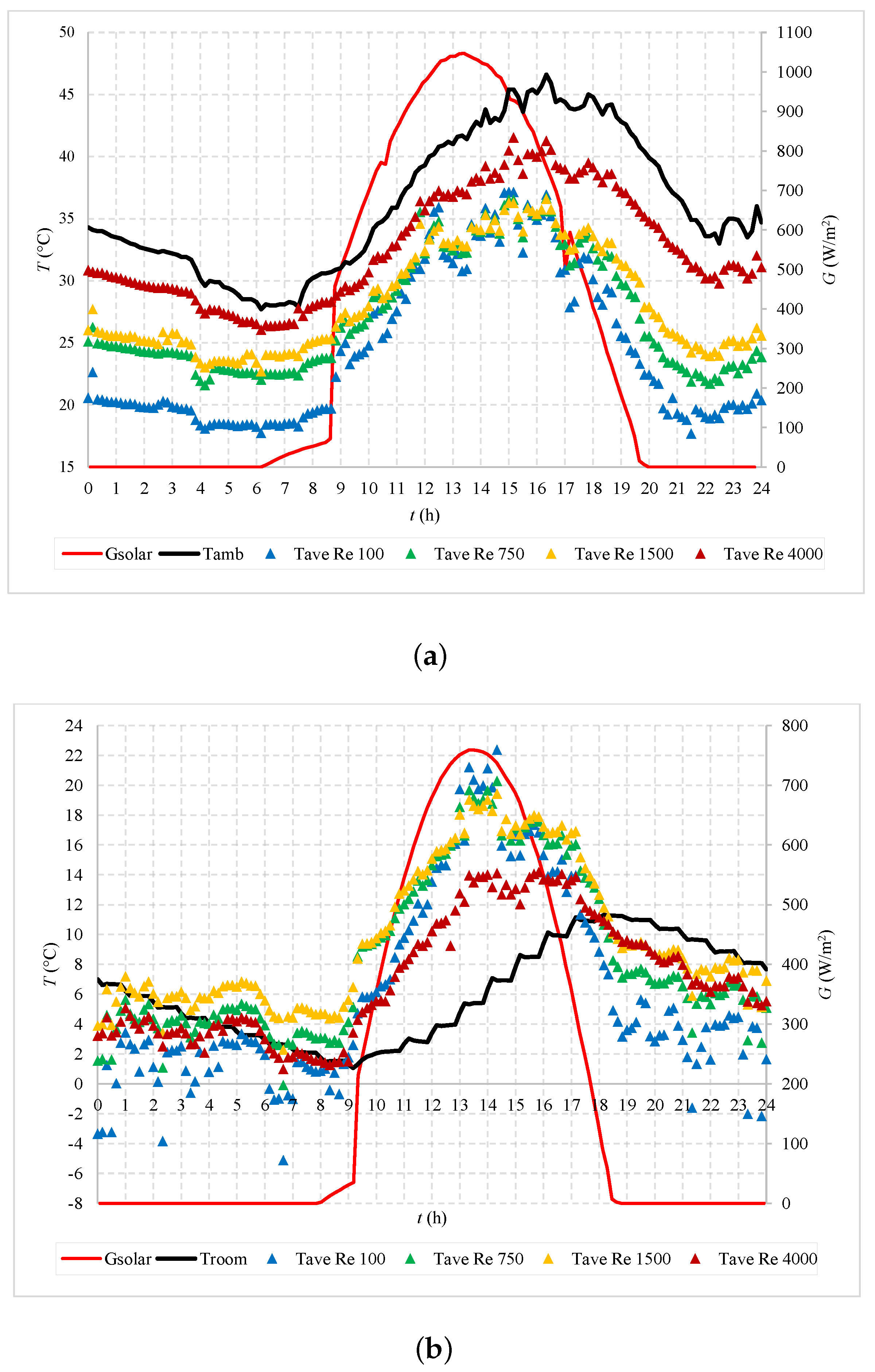
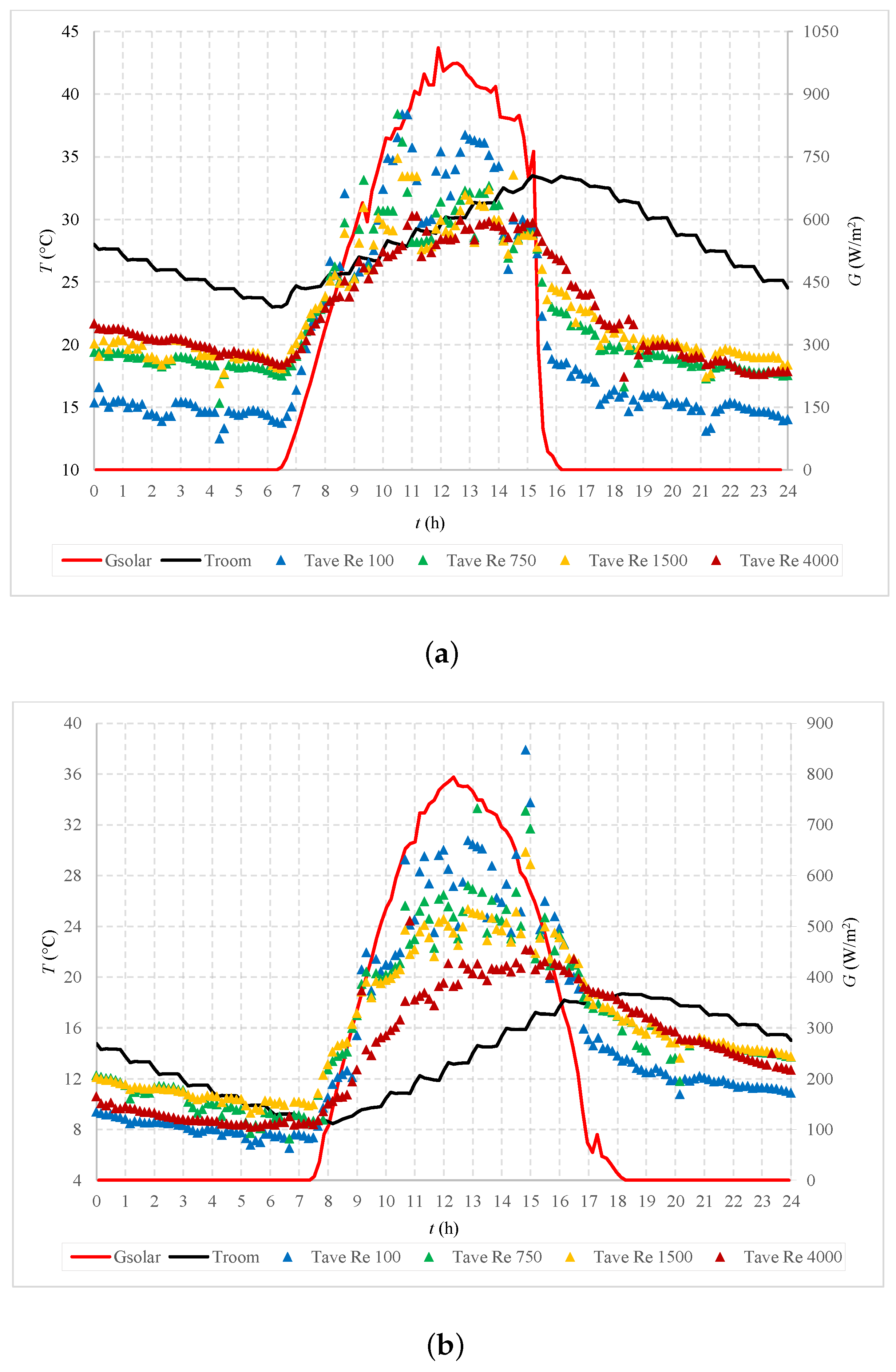
Figure 7a shows the comparison between the temperature of the air supplied by the EAHE and the indoor air temperature of the room in Juárez City. Throughout the warmest day, the air temperature supplied by the EAHE is lower than that reached by the room for all numbers. But, as is smaller, the temperature of the air supplied by the EAHE becomes colder than the indoor air. During the first hours, this temperature difference is close to 15 °C when = 100, which decreases as solar radiation increases after 9:00 h. However, this temperature difference reaches between 7 and 10 °C between 12:00 and 16:00 h. As solar radiation decreases, the supplied air recovers its cooling capacity for the rest of the day, reaching about 27 °C below the indoor room temperature, which provides up to 24 h of cooling effect.
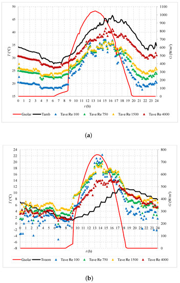
Figure 7.
Comparison between the temperature of the air supplied by the EAHE and the indoor air of the room in Juarez City: (a) warmest day and (b) coldest day.
On the coldest day in Juarez City, the EAHE supplies air at a temperature higher than the temperature of the room for most of the day for high Reynolds numbers (Figure 7b). During the first hours, a cooling effect is obtained by the system towards the room of up to 10 °C; however, as solar radiation increases, the heating effect of the system increases for all values, reaching a temperature difference of 15 °C between 9:00 h and 14:00 h. This temperature difference tends to decrease as the radiation decreases after 14:00 h, until a cooling effect is obtained again after 18:00 h, so a heating effect of between 9 and 18 h is obtained depending on the speed at which the air is driven by the EAHE.
Figure 8a presents the temperature of the air in the room and the air supplied by the EAHE in Zacualtipan. During the first hours of the day, a significant difference between both temperatures occurs (15 °C). But, during the hours with solar radiation, this difference decreases between 8:00 and 13:00 h, reaching a value between 3 and 5 °C, increasing again after 13:00 h. As solar radiation decreases, the effect of the air provided by the EAHE is cooling for the rest of the day, reaching a temperature difference of 20 °C. Thus, the supplied air temperature is colder than the air in the room the whole day.
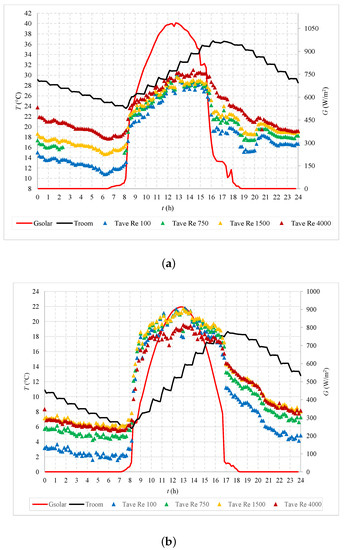
Figure 8.
Comparison between the temperature of the air supplied by the EAHE and the indoor air of the room in Zacualtipán: (a) warmest day and (b) coldest day.
Figure 8b shows that the air supplied by the EAHE during the first 8 h has a temperature lower than that of the room on the coldest day in Zacualtipán. As solar radiation increases, a heating effect begins after 8:00 h, reaching a temperature up to 11 °C greater than the indoor air between 8:00 and 13:00 h. Subsequently, once the radiation starts to decrease, a cooling effect occurs again from 16:00 h, with a temperature difference of between 6 and 10 °C, which can be harmful considering that the air in the room reaches values between 10 and 15 °C. The maximum temperature increase is 10.5 °C at 12:50 h, with a heating effect between 8:00 and 16:00 h.
The temperature of the air supplied by the EAHE and the indoor air temperature on the warmest day in Mexico City are presented in Figure 9a. The temperature of the air provided by the EAHE during the first hours of the day is between 7 and 12 °C lower than the room air temperature. However, in the hours of maximum solar radiation, between 8:00 and 15:00 h, the cooling effect decreases until the supplied air temperature is higher, between 5 and 10 °C, than the indoor air. As the day progresses and the radiation decreases, the cooling effect of the air supplied by the EAHE is recovered; the air supplied by the EAHE had a temperature between 10 and 16 °C lower than the indoor air.
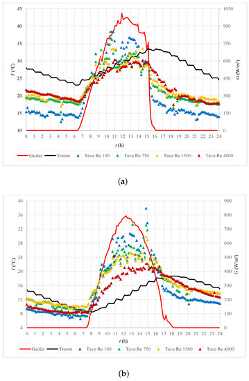
Figure 9.
Comparison between the temperature of the air supplied by the EAHE and the indoor air of the room in Mexico City: (a) warmest day and (b) coldest day.
On the coldest day, Figure 9b shows that when solar radiation is available, the temperature of the air supplied by the EAHE is warmer, between 12 and 18 °C (from 7:00 to 17:00 h), than the indoor air. On the other hand, for hours without solar radiation, the temperature of the supplied air is lower, between 2 and 5 °C, than that reached by the indoor air, which causes a cooling effect. The EAHE provided a heating operation time of 10 h.
Table 6 summarizes the running schedules of the EAHE in the four cities analyzed in this work for the different values of . The table presents the hours in which the EAHE works well on the warmest day and the hours in which the EAHE works well on the coldest day. These data are presented in the column labeled working time (W.T.). The table also presents the schedules in which the EAHE complies with its cooling and heating duty for the warmest and coldest days, respectively.
Table 6.
Running schedules of the EAHE in the different cities (W.T. = working time).
6.2. Results of the Simulations of the EAHE Connected to the Building Room
This section presents the analysis of the EAHE connected to a room. The effect of EAHE on the indoor air temperature of the room and its cooling and heating thermal loads is presented here. Such results were obtained by coupling each city’s CFD model of the EAHE and the BES room model.
As mentioned in previous sections, three input data are needed to feed the VENTILATION component in TRNSYS: rate of air changes, the temperature of the air from the EAHE that is injected into the house, and relative humidity. The air change ratio () was calculated according to [64]:
The volumetric flow rate is the product of the average velocity of the fluid at the outlet of the EAHE () and the area of the pipe (A). This volumetric flow is divided by the total volume of the room, in this case, a space of 20.52 m. Table 7 reports the values for each Reynolds number with different numbers of pipes implemented for a room. It is worth mentioning that pipe layout is such that no thermal interference between pipes occurs. The value obtained with one pipe was multiplied by the number of lines to obtain the for more pipes. As expected, the increases as the number of pipes and the Reynolds number increase. The peak = 3.1 1/h is achieved for 20 pipes and = 4000.
Table 7.
Air change ratio (1/h) as a function of air velocity for different numbers of pipes.
The effect of EAHE with 5, 10, 15, and 20 pipes on the thermal loads of the room was simulated. The maximum number of pipes was selected according to the area of the room (8.55 m2). As the number of pipes increases, the airflow into the room increases. This is done to increase the and improve the indoor conditions of the room. The airflow from the EAHE is supplied to Room B, as shown in Figure 3. The results from simulations of the EAHE connected to the room are presented below. It is worth mentioning that on a warm day, the EAHE only provides air to the room when the supplied air temperature is lower than that of indoor air, while for the coldest day, the EAHE only provides air to the room during the hours when the supplied air is warmer than the indoor air. It is supposed that the outlet of the EAHE is closed when this system does not comply with its duty of cooling or heating when required; in this way, it is avoided by introducing warm air on the warmest day and cold air on the coldest day. Due to restrictions of the numerical code, it is suitable for laminar and transitional flow only, but if it is required to use high air velocities or turbulent regime to achieve a high air change ratio (), it could not provide reliable results. Thus, it was decided to increase the number of pipes to determine the amount of ACR necessary to generate a significant air change ratio within the room. Implementing 20 pipes in an area of 8.55 m2 to obtain an air change value that generates a significant effect within the room could be somewhat difficult to carry out; however, within a real system, it is possible to obtain the same maximum value of ACR reported in the study, modifying specific EAHE parameters such as air velocity and pipe diameter to increase volumetric flow, which results in fewer pipes for the same value. On the other hand, according to the research developed by Minaei and Rabani [65], it is considered that a separation distance greater than 15 cm does not significantly affect the temperature at the outlet of the EAHE, so if someone wants to implement 20 pipes in the room, 10 pipes can be grouped on the south wall and 10 pipes on the east wall with a separation distance of 15 cm, covering a length of 2.4 m on each side. Another factor that is worth mentioning is the soil thermal saturation. When the EAHE is working, the temperature of the soil surrounding the pipes could increase as time goes on, then after a period between 6 and 12 h of continuous operation, the soil becomes thermally saturated and it could affect the performance of the EAHE [9]. The soil thermal saturation was not addressed in this work, but it should be considered when intermittent EAHE use is recommended.
Table 8 presents the maximum and minimum indoor air temperatures of the building room without EAHE obtained with TRNSYS and both temperatures when the EAHE is connected to the building room obtained with a CFD-BES coupling. The table presents results for airflow with = 4000, and it is supposed that twenty pipes are connected to the building room for all cities. Further, the temperature difference () between the indoor air temperature of the room without EAHE and with EAHE is also presented. A high Reynolds value was chosen because a high velocity of the airflow supplied by the EAHE favors its mixing with the room’s indoor air.
Table 8.
Maximum indoor air temperature difference of the room without and with EAHE considering 20 pipes and = 4000.
On the warmest day, the values of for the different cities range between 1.7 and 3.2 °C. The indoor air temperature reduction provided by the EAHE appears to be small, but it is worth mentioning that the room is closed and does not have other infiltration. Although infiltration is a relevant parameter, especially for having a healthy indoor environment, here, infiltration, other than the air introduced by the EAHE into the room, was not considered, because this research aims to focus on the influence of the EAHE on the indoor air temperature of the room. Thus, the indoor air temperature of the room without EAHE and the corresponding temperature of a room with EAHE were compared. Thus, leaving out other parameters could give a better understanding of the behavior of the air in the room with the two conditions mentioned above. In Monterrey, the EAHE was able to reduce the indoor air temperature by 3.2 °C, which is the maximum temperature reduction of all cities. The second more significant temperature reduction occurred in Juárez City with a value of 2.8 °C. Then, Zacaltipán had a temperature reduction of 2.6 °C. Finally, in Mexico City, the EAHE reduced the indoor air temperature by up to 1.7 °C. Thus, on warm days, buildings situated in cities in Mexico benefit from installing EAHE because the indoor air temperature is decreased.
On the other hand, Table 8 also shows the values of for the coldest day of the different cities. The values of ranged between 1.2 and 3.5 °C. In Juárez City, where indoor air reached the lowest value, the EAHE increased indoor air temperature by 3.5 °C. The second more significant temperature increase occurred in Mexico City with a value of 2.3 °C. Finally, the indoor air temperature increase provided by the EAHE in Zacaltipán (1.2 °C) was very similar to that in Monterrey (1.3 °C).
The EAHE connected to a building room can influence the thermal load required to condition the room space. Because the most significant effect on temperature is obtained with the airflow supplied by 20 pipes for the different Reynolds numbers, the cooling and heating loads of the room with EAHE with 20 pipes are presented here.
Table 9 shows the cooling load of the warmest day for each city under study. The values of the cooling load indicate that the thermal load decreases when airflow increases with velocity. The most significant cooling load reduction occurred in Zacualtipán, 2.39 kWh, which is equal to a 6% reduction. The second more significant cooling load reduction was obtained for the room in Monterrey and Juárez City, where the cooling load reductions were similar, with values of 1.64 kWh and 1.61 kWh, respectively. Both values also represent a 2% cooling load reduction. Finally, a minor decrease occurred in Mexico City, with 0.86 kWh (3%). The cooling load reductions are relatively small, but it should be remembered that these values belong to just one day. Depending on the number of days of the year that need cooling in each type of climate, the EAHE could reduce significantly the annual cooling load. Although the previous reductions are small, the year-round savings could be important depending on the type of climate in which the EAHE is installed. Future research should consider the year-round performance of EAHE connected to the building room.
Table 9.
Cooling loads (kWh) for the warmest day.
Table 10 presents the heating loads of the building room on the coldest day of the year 2020. The table demonstrates an EAHE with 20 pipes, and = 4000 provides the most significant room heating load reduction. When the EAHE is installed in the building room in Mexico City, it provided the most significant heating load reduction; it was reduced by 3.51 kWh (11%). In Zacualtipán, the EAHE reduced the heating load by 2.11 kWh, equivalent to 5%. In Juárez City, the heating load was reduced by 0.49 kWh (2%). In Monterrey, the EAHE reduced the heating load by just 0.16 kWh (0.3%). As in the cooling loads, the heating load reductions might be small, but these values belong to just one day. Depending on the number of days of the year that need heating, the EAHE could reduce significantly the annual heating load.
Table 10.
Heating loads (kWh) for the coldest day.
7. Conclusions
A simulation method that couples BES and CFD was used to simulate the thermal behavior of an EAHE connected to a building room in four cities with different climates in Mexico. Simulations were performed for the warmest and the coldest days of 2020, and the following is concluded:
- The comparison of the indoor air temperature and the temperature of the air at the outlet of the EAHE allowed us to understand the hours in which the EAHE works well and in which it does not work for each of the four cities. On the warmest day, the EAHE could supply air with a lower temperature than indoor air of the room for 24 h in Monterrey, Juárez City, and Zacualtipán. The EAHE worked well for 18 h in Mexico City.
- On the coldest day, Juárez City, Monterrey, Mexico City, and Zacualtipán require heating, and the EAHE could supply air with a higher temperature than indoor air for 24 h, 17 h, 10 h, and 8 h, respectively.
- It was found that the indoor air temperature conditions improved due to installing the EAHE with 20 pipes. On the warmest day, the EAHE decreased the indoor air temperature by a factor between 1.7 and 3.2 °C. On the coldest day, the EAHE increased the indoor air temperature between 1.5 and 3.5 °C.
- The effect of connecting an EAHE on the daily heating and cooling loads of the building room was also analyzed. On the warmest day, the EAHE reduced the cooling load of the room between 2% and 6%. On the coldest day, the EAHE reduced the heating load by a factor between 0.3% and 11%. Although the previous reductions are small, the year-round savings could be important depending on the type of climate in which the EAHE is installed.
Future research should consider the year-round performance of EAHE connected to the building room in the different types of climates in Mexico. Further, the payback period of the EAHE should be found in order to determine in which locations it is feasible to install EAHE for improving indoor environment conditions. Finally, the soil thermal saturation was not addressed in this work, but it should be considered when intermittent EAHE use is recommended.
Author Contributions
Conceptualization, I.H.-P., M.R.-V., Y.C.; writing—original draft preparation, M.R.-V., I.H.-P., I.H.-L., Y.C., C.M.J.-X., L.A.B.-T. and A.A.-A.; writing—review and editing, I.H.-P., M.R.-V., C.M.J.-X., L.A.B.-T. and A.A.-A.; supervision, I.H.-P., I.H.-L. and Y.C. All authors have read and agreed to the published version of the manuscript.
Funding
This research received no external funding.
Data Availability Statement
The data used to support the findings of this study are available from the corresponding author upon request.
Acknowledgments
The authors acknowledge the Nacional-Comisión Nacional del Agua (SMN-CONAGUA) for sharing the climatic data of the different cities. The authors dedicate this work to the memory of our mentor and friend Jesús Xamán, who guided us to develop this work and encouraged everybody when we needed it.
Conflicts of Interest
The authors declare no conflict of interest.
Abbreviations
| BES | building energy simulation |
| CFD | computational fluid dynamics |
| EAHE | Earth-to-Air Heat Exchanger |
| Nomenclature | |
| A | area, m |
| air change ratio, 1/h | |
| convective energy between air and soil, W/m·K | |
| specific heat, kJ/(kg·K) | |
| , | Body forces (N/m) |
| G | solar radiation, W/m |
| h | convective heat transfer coefficient, W/(m K) |
| number of nodes in direction x | |
| number of nodes in direction y | |
| relative humidity, % | |
| latent heat flux due to evaporation, W/(m K) | |
| long wavelength radiation, W/m | |
| P | pressure, Pa |
| Reynolds number | |
| short wavelength radiation, W/m | |
| t | time, s |
| T | temperature, °C |
| u, v | components of velocity, m/s |
| V | volume, m |
| volumetric flow rate, m/s | |
| x, y | coordinates, m |
| Greek | |
| thickness of thermal insulation | |
| solar absorptance | |
| thermal conductivity, W/(m·K) | |
| thermal emittance | |
| dynamic viscosity (N·s/m) | |
| density, kg/m | |
| Subscripts | |
| ambient | |
| average | |
| conduction | |
| convection | |
| evaporation | |
| surface | |
| wind |
References
- D’Agostino, D.; Greco, A.; Masselli, C.; Minichiello, F. The employment of an earth-to-air heat exchanger as pre-treating unit of an air conditioning system for energy saving: A comparison among different worldwide climatic zones. Energy Build. 2020, 229, 11051. [Google Scholar] [CrossRef] [PubMed]
- Rosa, N.; Santos, P.; Costa, J.J.; Gervásio, H. Modelling and performance analysis of an earth-to-air heat exchanger in a pilot installation. J. Build. Phys. 2018, 45, 259–287. [Google Scholar] [CrossRef]
- Bisoniya, T.S.; Kumar, A.; Baredar, P. Heating potential evaluation of earth–air heat exchanger system for winter season. J. Build. Physics 2015, 39, 242–260. [Google Scholar] [CrossRef]
- Peretti, C.; Zarrella, A.; De Carli, M.; Zecchin, R. The design and environmental evaluation of earth-to-air heat exchangers (EAHE): A literature review. Renew. Sustain. Energy Rev. 2013, 28, 107–116. [Google Scholar] [CrossRef]
- Agrawal, K.K.; Misra, R.; Das Agrawal, G. Improving the thermal performance of ground air heat exchanger system using sand-bentonite (in dry and wet condition) as backfilling material. Renew. Energy 2020, 146, 2008–2023. [Google Scholar] [CrossRef]
- Cuny, M.; Lapertot, A.; Lin, J.; Kadoch, B.; Le Metayer, O. Multi-criteria optimization of an earth-air heat exchanger for different French climates. Renew. Energy 2020, 157, 342–352. [Google Scholar] [CrossRef]
- Lin, Y.; Feng, H.; Yang, W.; Hao, X.; Tian, L.; Yuan, X. Thermal performance optimization of a semi-nested building coupled with an earth-to-air heat exchanger using iterative Taguchi method. Renew. Energy 2022, 195, 1275–1290. [Google Scholar] [CrossRef]
- Sakhri, N.; Menni, Y.; Ameur, H. Experimental investigation of the performance of earth-to-air heat exchangers in arid environments. J. Arid Environ. 2020, 180, 104215. [Google Scholar] [CrossRef]
- Belloufi, Y.; Zerouali, S.; Rouag, A.; Aissaoui, F.; Atmani, R.; Brima, A.; Moummi, N. Transient assessment of an earth air heat exchanger in warm climatic conditions. Geothermics 2022, 180, 102442. [Google Scholar] [CrossRef]
- Sakhri, N.; Menni, Y.; Ameur, H. Effect of the pipe material and burying depth on the thermal efficiency of earth-to-air heat exchangers. Case Stud. Chem. Environ. Eng. 2022, 2, 100013. [Google Scholar] [CrossRef]
- Atwany, H.; Hamdan, M.O.; Bassam, A.; Alami, A.H.; Attom, M. Experimental evaluation of ground heat exchanger in UAE. Renew. Energy 2020, 159, 538–546. [Google Scholar] [CrossRef]
- Agrawal, K.K.; Bhardwaj, M.; Misra, R.; Agrawal, G.D.; Bansal, V. Optimization of operating parameters of earth air tunnel heat exchangers for space cooling: Taguchi method approach. Geotherm. Energy 2018, 6, 1–17. [Google Scholar] [CrossRef]
- Díaz-Hernández, H.P.; Macias-Melo, E.V.; Aguilar-Castro, K.M.; Hernández-Pérez, I.; Xamán, J.; Serrano-Arellano, J.; López-Manrique, L.M. Experimental study of an earth to air heat exchanger (EAHE) for warm humid climatic conditions. Geothermics 2020, 84, 101741. [Google Scholar] [CrossRef]
- Kharbouch, A.; Berrabah, S.; Bakhouya, M.; Gaber, J.; El Ouadghiri, D.; Idrissi Kaitouni, S. Experimental and Co-Simulation Performance Evaluation of an Earth-to-Air Heat Exchanger System Integrated into a Smart Building. Energies 2022, 15, 5407. [Google Scholar] [CrossRef]
- Ahmed, S.F.; Khan, M.M.K.; Amanullah, M.T.O.; Rasul, M.G.; Hassan, N.M.S. Thermal performance of building-integrated horizontal earth-air heat exchanger in a subtropical hot humid climate. Geothermics 2022, 99, 102313. [Google Scholar] [CrossRef]
- Kaushal, M. Performance analysis of clean energy using geothermal earth to air heat exchanger (GEAHE) in Lower Himalayan Region—Case study scenario. Energy Build. 2021, 248, 111166. [Google Scholar] [CrossRef]
- Li, H.; Ni, L.; Liu, G.; Yao, Y. Performance evaluation of Earth to Air Heat Exchanger (EAHE) used for indoor ventilation during winter in severe cold regions. Appl. Therm. Eng. 2019, 160, 114111. [Google Scholar] [CrossRef]
- Li, H.; Ni, L.; Yao, Y.; Sun, C. Annual performance experiments of an earth-air heat exchanger fresh air-handling unit in severe cold regions: Operation, economic and greenhouse gas emission analyses. Renew. Energy 2020, 146, 25–37. [Google Scholar] [CrossRef]
- Pakari, A.; Ghani, S. Performance evaluation of a near-surface earth-to-air heat exchanger with short-grass ground cover: An experimental study. Energy Convers. Manag. 2019, 201, 112163. [Google Scholar] [CrossRef]
- Zeitoun, W.; Lin, J.; Siroux, M. Energetic and exergetic analyses of an experimental Earth–Air Heat Exchanger in the northeast of France. Energies 2023, 16, 1542. [Google Scholar] [CrossRef]
- Yang, Q.; Hu, Z.; Tao, Y.; Shi, L.; Tu, J.; Chai, J.; Wang, Y. Experimental and numerical study on cooling performance of a novel earth-to-air heat exchanger system with an inlet plenum chamber. Energy Convers. Manag. 2023, 277, 116671. [Google Scholar] [CrossRef]
- Mihalakakou, G.; Santamauris, M.; Lewis, J.O.; Asimakopoulos, D.N. On the application of the energy balance equation to predict ground temperature profiles. Sol. Energy 1997, 60, 181–190. [Google Scholar] [CrossRef]
- Pakari, A.; Ghani, S. Numerical evaluation of the thermal performance of a near-surface earth-to-air heat exchanger with short-grass ground cover: A parametric study. Int. J. Ref. 2021, 125, 25–33. [Google Scholar] [CrossRef]
- Cuny, M.; Lin, J.; Siroux, M.; Fond, C. Influence of rainfall events on the energy performance of an earth-air heat exchanger embedded in a multilayered soil. Renew. Energy 2020, 147, 2664–2675. [Google Scholar] [CrossRef]
- Hermes, V.F.; Ramalho, J.V.A.; Rocha, L.A.O.; dos Santos, E.D.; Marques, W.C.; Costi, J.; Rodrigues, M.K.; Isoldi, L.A. Further realistic annual simulations of earth-air heat exchangers installations in a coastal city. Sustain. Energy Technol. Assess. 2020, 37, 100603. [Google Scholar] [CrossRef]
- Larwa, B.; Kupiec, K. Heat transfer in the ground with a horizontal heat exchanger installed–Long-term thermal effects. Appl. Therm. Eng. 2020, 164, 114539. [Google Scholar] [CrossRef]
- Mehdid, C.E.; Benchabane, A.; Rouag, A.; Moummi, N.; Melhegueg, M.A.; Moummi, A.; Benabdi, M.L.; Brima, A. Thermal design of Earth-to-air heat exchanger. Part II: A new transient semi-analytical model and experimental validation for estimating air temperature. J. Clean. Prod. 2018, 198, 1536–1544. [Google Scholar] [CrossRef]
- Beenzama, M.H.; Menhoudj, S.; Mokhtari, A.M.; Lachi, M. Comparative study of the thermal performance of an earth air heat exchanger and seasonal storage systems: Experimental validation of Artificial Neural Networks model. J. Energy Storage 2022, 53, 105177. [Google Scholar] [CrossRef]
- Long, T.; Zhao, N.; Li, W.; Wei, S.; Li, Y.; Lu, Y.; Huang, S.; Qiao, Z. Numerical simulation of diurnal and annual performance of coupled solar chimney with earth-to-air heat exchanger system. J. Energy Storage 2022, 48, 104037. [Google Scholar] [CrossRef]
- Gou, X.; Wei, H.; He, X.; Du, J.; Yang, D. Experimental evaluation of an earth–to–air heat exchanger and air source heat pump hybrid indoor air conditioning system. Energy Build. 2022, 256, 111752. [Google Scholar]
- Gou, X.; Wei, H.; He, X.; He, M.; Yang, D. Integrating phase change material in building envelopes combined with the earth-to-air heat exchanger for indoor thermal environment regulation. Build. Environ. 2022, 221, 109318. [Google Scholar]
- Akhtari, M.R.; Shayegh, I.; Karimi, N. Techno-economic assessment and optimization of a hybrid renewable earth-air heat exchanger coupled with electric boiler, hydrogen, wind and PV configurations. Renew. Energy 2020, 148, 839–851. [Google Scholar] [CrossRef]
- Hamdane, S.; Pires, L.C.C.; Silva, P.D.; Gaspar, P.D. Evaluating the Thermal Performance and Environmental Impact of Agricultural Greenhouses Using Earth-to-Air Heat Exchanger: An Experimental Study. Appl. Sci. 2023, 13, 1119. [Google Scholar] [CrossRef]
- Wei, H.; Yang, D.; Guo, Y.; Chen, M. Coupling of earth-to-air heat exchangers and buoyancy for energy efficient ventilation of buildings considering Dynamic thermal behavior and cooling/heating capacity. Energy 2018, 147, 587–602. [Google Scholar] [CrossRef]
- Yang, D.; Wei, H.; Shi, R.; Wang, J. A demand-oriented approach for integrating earth-to-air heat exchangers into buildings for achieving year-round indoor thermal comfort. Energy Convers. Manag. 2019, 182, 95–107. [Google Scholar] [CrossRef]
- Misra, R.; Jakhar, S.; Agrawal, K.K.; Sharma, S.; Jamuwa, D.K.; Soni, M.S.; Agrawal, G.D. Field investigations to determine the thermal performance of earth air tunnel heat exchanger with dry and wet soil: Energy and Exergetic Analysis. Energy Build. 2018, 171, 107–115. [Google Scholar] [CrossRef]
- Aranda-Arizmendi, A.; Rodríguez-Vázquez, M.; Jiménez-Xamán, C.M.; Romero, R.J.; Montiel-González, M. Parametric Study of the Ground-Air Heat Exchanger (GAHE): Effect of Burial Depth and Insulation Length. Fluids 2023, 8, 40. [Google Scholar] [CrossRef]
- Minaei, A.; Safikhani, H. A new transient analytical model for heat transfer of earth-to-air heat exchangers. J. Build. Eng. 2021, 33, 101560. [Google Scholar] [CrossRef]
- Qi, D.; Li, S.; Zhao, C.; Xie, W.; Li, A. Structural optimization of multi-pipe earth to air heat exchanger in greenhouse. Geothermics 2022, 98, 102288. [Google Scholar] [CrossRef]
- Papakostas, K.T.; Tsamitros, A.; Martinopoulos, G. Validation of modified one-dimensional models simulating the thermal behavior of earth-to-air heat exchangers—Comparative analysis of modelling and experimental results. Geothermics 2019, 82, 1–6. [Google Scholar] [CrossRef]
- Amanowicz, L.; Wojtkowiak, J. Thermal performance of multi-pipe earth-to-air heat exchangers considering the non-uniform distribution of air between parallel pipes. Geothermics 2020, 88, 101896. [Google Scholar] [CrossRef]
- Asgari, B.; Habibi, M.; Hakkaki-Fard, A. Assessment and comparison of different arrangements of horizontal ground heat exchangers for high energy required applications. Appl. Therm. Eng. 2020, 167, 114770. [Google Scholar] [CrossRef]
- Amanowicz, L.; Wojtkowiak, J. Validation of CFD model for simulation of multi-pipe earth-to-air heat exchanger (EAHEs) flow performance. Therm. Sci. Eng. Progress 2018, 5, 44–49. [Google Scholar] [CrossRef]
- Ahmad, H.; Sakhri, N.; Menni, Y.; Omri, M.; Ameur, H. Experimental study of the efficiency of earth-to-air heat exchangers: Effect of the presence of external fans. Case Stu. Therm. Eng. 2021, 28, 101461. [Google Scholar] [CrossRef]
- Yusof, T.M.; Ibrahim, H.; Azmi, W.H.; Rejab, M.R.M. The thermal characteristics and performance of a ground heat exchanger for tropical climates. Renew Energy 2018, 121, 528–538. [Google Scholar] [CrossRef]
- Maytorena, V.M.; Hinojosa, J.F. Thermal Analysis of a Generic Earth-to-Air Heat Exchanger Coupled with a Room during the Summer Season in a Desert Climate. J. Energy Eng. 2022, 148, 04022001. [Google Scholar] [CrossRef]
- Skotnicka-Siepsiak, A. An Evaluation of the Performance of a Ground-to-Air Heat Exchanger in Different Ventilation Scenarios in a Single-Family Home in a Climate Characterized by Cold Winters and Hot Summers. Energies 2022, 15, 105. [Google Scholar] [CrossRef]
- Long, T.; Zhao, N.; Li, W.; Wei, S.; Li, Y.; Lu, Y.; Huang, S.; Qiao, Z. Benefits of integrating phase-change material with solar chimney and earth-to-air heat exchanger system for passive ventilation and cooling in summer. Appl. Therm. Eng. 2022, 214, 118851. [Google Scholar] [CrossRef]
- Xamán, J.; Hernández-Pérez, I.; Arce, J.; Álvarez, G.; Ramírez-Dávila, L.; Noh-Pat, F. Numerical study of earth-to-air heat exchanger: The effect of thermal insulation. Energy Build. 2014, 85, 356–361. [Google Scholar] [CrossRef]
- Xamán, J.; Hernández-López, I.; Alvarado-Juárez, R.; Hernández-Pérez, I.; Álvarez, G.; Chávez, Y. Pseudo transient numerical study of an earth-to-air heat exchanger for different climates of Mexico. Energy Build. 2015, 99, 273–283. [Google Scholar] [CrossRef]
- Rodríguez-Vázquez, M.; Xamán, J.; Chávez, Y.; Hernández-Pérez, I.; Simá, E. Thermal potential of a geothermal earth-to-air heat exchanger in six climatic conditions of México. Mech. Ind. 2020, 21, 308. [Google Scholar] [CrossRef]
- Gauthier, C.; Lacroix, M.; Bernier, H. Numerical simulation of soil heat exchanger-storage systems for greenhouses. Sol. Energy 1997, 60, 333–346. [Google Scholar] [CrossRef]
- National Council for Dwellings, Code for Buildings. (3rd Edition). Available online: https://www.gob.mx/conavi (accessed on 1 February 2023). (In Spanish)
- Hollmuller, P. Analytical characterisation of amplitude-dampening and phase-shifting in air/soil heat-exchangers. Int. J. Heat Mass Transf. 2003, 46, 4303–4317. [Google Scholar] [CrossRef]
- Khabbaz, M.; Bengamou, B.; Limam, K.; Hollmuller, P. Experimental and numerical study of n earth-to-air heat exchanger for air cooling in a residential building in hot semi-arid climate. Energy Build. 2016, 125, 109–121. [Google Scholar] [CrossRef]
- Badescu, V. Simple and accurate model for the ground heat exchanger of a passive house. Renew. Energy 2007, 32, 845–855. [Google Scholar] [CrossRef]
- Patankar, S. Numerical Heat Transfer and Fluid Flow; Taylor & Francis: Abingdon, UK, 1980. [Google Scholar]
- Van Doormaal, J.; Raithby, G. Enhancements of the SIMPLE method for predicting incompressible fluid flow. Numer. Heat Trans. 1984, 7, 147–163. [Google Scholar]
- House, J.M.; Beckermann, C.; Smith, T.F. Effect of a centered conducting body on natural convection heat transfer in an enclosure. Numer. Heat Trans. 1990, 18, 213–225. [Google Scholar] [CrossRef]
- Ramírez-Dávila, L.; Xamán, J.; Arce, J.; Álvarez, G.; Hernández-Pérez, I. Numerical study of earth-to-air heat exchanger for three different climates. Energy Build. 2014, 76, 238–248. [Google Scholar] [CrossRef]
- Rodríguez-Vázquez, M.; Hernández-Pérez, I.; Xamán, J.; Chávez, Y.; Gijón-Rivera, M.; Belman-Flores, J.M. Coupling building energy simulation and computational fluid dynamics: An overview. J. Build. Phys. 2020, 44, 137–180. [Google Scholar] [CrossRef]
- Díaz-Rodríguez, J.A. Los suelos lacustres de la ciudad de México. Rev. Int. Desastr. Nat. Accid. Infraestruct. Civ. 2006, 6, 111–130. [Google Scholar]
- Instituto Nacional de Estadistica y Geografia, Prontuario de Información geográFica Municipal de los Estados Unidos Mexicanos. Mexico City. INEGI. 2009. Available online: https://www.inegi.org.mx (accessed on 25 March 2022).
- American Society of Heating and Refrigerating and Air-Conditioning Engineers. ASHRAE Handbook of Fundamentals; American Society of Heating and Refrigerating and Air-Conditioning Engineers, Inc.: Peachtree Corners, GA, USA, 2009. [Google Scholar]
- Minaei, A.; Rabani, R. Development of a transient analytical method for multi-pipe earth-to-air heat exchangers with parallel configuration. J. Build. Eng. 2023, 73, 106781. [Google Scholar] [CrossRef]

Disclaimer/Publisher’s Note: The statements, opinions and data contained in all publications are solely those of the individual author(s) and contributor(s) and not of MDPI and/or the editor(s). MDPI and/or the editor(s) disclaim responsibility for any injury to people or property resulting from any ideas, methods, instructions or products referred to in the content. |
© 2023 by the authors. Licensee MDPI, Basel, Switzerland. This article is an open access article distributed under the terms and conditions of the Creative Commons Attribution (CC BY) license (https://creativecommons.org/licenses/by/4.0/).