Bridging Law Application to Fracture of Fiber Concrete Containing Oil Shale Ash

Abstract

Concrete is a widely used material in various industries, including hazardous waste management. At the same time, its production creates a significant carbon footprint. Therefore, intensive research is being conducted to create more eco-friendly concrete, for example, partially replacing cement with by-products such as oil shale ash (OSA) or improving properties by adding dispersed fibers such as basalt fibers (BFs). The article consists of experimental testing of nine types of concrete and the modeling of crack propagation in bending. The basic trends of crack propagation in samples of concrete with OSA and BFs are simulated using a two-dimensional Finite Element (FE) model considering only material degradation on the opening crack surface and experimental data of three- and four-point bending tests. Crack propagation is modeled using the bridging law approach. A surrogate model for predicting the peak loading as a function of tensile strength and fracture work was created. An examination of the results of the FE model shows that the bilinear and nonlinear bridging law functions best describe the crack growth in the analyzed material. A comparison of experimental and modeled results showed that the length of the composite BF strongly affects the accuracy of the numerical model.

1. Introduction

Concrete is the second most used substance in the world after water [1], despite cement, one of its main compounds, being responsible for more than 7% of global carbon dioxide emissions [2]. Therefore, possibilities for producing environmentally friendly concrete have been actively studied in recent years. In 1968, Sweden was the first country to suggest to the United Nations a conference focused on human interaction with the environment, which resulted in The United Nations Conference on the Human Environment held in Stockholm in 1972. The Earth Summit in 1992, held in Rio de Janeiro, followed by the Kyoto Protocol in 1997, established a policy to protect our environment and support development. The latest international treaty on climate change is the Paris Agreement signed in 2016, which significantly accelerated the shift in human behavior and industry awareness of greenhouse gas production and resource depletion. Recent trends support the circular economy and circular material flow. In the case of concrete, the use of supplementary cementitious materials (SCM) as a cement replacement, and the use of secondary fuel resources for cement production, has significantly impacted cement’s carbon footprint. The use of secondary raw materials/industrial side streams as supplementary materials fits well with the circular economy concept and helps solve the problems of climate change and environmental degradation. However, their widespread use is limited by several other factors, such as the need for more suitable applications in place and the amount of SCM locally available [3].

Adding oil shale ash (OSA) to concrete has clear advantages in reducing the use of raw materials during concrete production. At the same time, this approach helps to make good use of OSA, a byproduct of energy production generated in huge amounts due to oil shale combustion processes. The cement replacement level with fly ash is limited to 35% of the cement mass in the concrete [4]. A promising approach is using OSA instead of fly ash as an immobilizing matrix in hazardous waste management. Analysis of mineral composition and cementation properties have shown that OSA may be used as a barrier material to immobilize hazardous materials in its matrix. Studies of the leaching characteristics of concrete with OSA show that the fraction of readily soluble inorganic components decreases during curing time, and the mobility of potentially dangerous elements does not increase [5]. It should also be noted that concrete with OSA has a lower early age strength than concrete containing exclusively Ordinary Portland Cement.

The excellent mechanical properties of fiber-reinforced concrete are the reason for the growing interest in its research and application in hazardous waste’s short-term and long-term storage [6]. The beneficial effects of fibers in improving post-cracking strength and energy absorption capacity are attributed to their ability to transfer tensile stress across cracks, known as the crack-bridging effect [7]. Basalt fibers (BFs) in concrete have been found to have better properties (high tensile strength, and chemical and heat resistance) and higher economic efficiency than other fibers [8,9,10]. The use of basalt fiber as a reinforcement for improving the mechanical properties of composite materials has been widely studied [11,12,13].

Concrete usually contains discontinuities such as cracks and voids that dominate the material’s strength, deformability, and failure behavior. The initiation, propagation, and coalescence of cracks lead to the degradation of the mechanical behavior of concrete. Therefore, it is essential to understand the cracking behavior of concrete to ensure the reliable performance of structures [14]. Safety assessment of concrete structures used in hazardous waste management applications requires realistic models to reproduce the behavior of the materials.

The Finite Element (FE) method [15,16] has become a mainstream tool in various engineering fields, such as mechanical and civil engineering, biomedical engineering, and material science. FE is also a useful tool for modeling the mechanical properties of concrete. Khormani et al. [17] estimated the compressive strength of concrete using a 3D mesoscale finite element model created with the help of computed tomography (CT) images. The quality of the images obtained from the CT scanner allows for modeling the two types of aggregates used based on the brightness range of each aggregate. Carvalho et al. [7] used the finite element method to capture fibers’ bridging effect in a four-point bending test. They use a discrete crack approach to modeling, requiring material parameters usually available in design codes and technical data sheets. A three-point bending test for high-performance concrete reinforced with short steel hook-end Dramix fibers under a 2D plane stress condition is simulated by Le et al. [18]. Fiber bridging and cohesion resistance are used as fundamental mechanisms for the development of fiber-reinforced concrete models. The evolution of complex cracks, including tree-shaped cracks, regularly distributed intersecting cracks, and randomly distributed intersecting cracks, is simulated and studied by Jia [14] using the field-enriched finite element method.

Although the well-established and widely used FE method is the dominant numerical tool for solving fracture mechanics problems, other approaches are also described in the literature; for example, the boundary element method is relatively widely used [19,20]. Jiang et al. [21] demonstrate material analysis with interfacial cracks using the finite difference method. Simulations of Brazilian disc and compressive tests with the discrete element method are described in [22,23].

There are many numerical models for characterizing the initiation and propagation of cracks in concrete. One of the first nonlinear crack models to analyze the failure process of concrete was the cohesive crack model [24,25,26]. Recently, phase field theory has been increasingly used for simulations of crack initiation, propagation, merging, and branching [27,28,29]. Feng et al. [30] demonstrate the successful application of the phase-field regularized cohesive crack model to simulate the three-point bending test for concrete. On the other hand, Li et al. [31] offer to combine the phase-field regularized cohesive zone model and random aggregate models for simulating complicated mesoscale damage and fractures. Fiber-bridging constitutive law applications have been studied in [32,33].

Considering the rapidly growing availability of computing resources, there is a tendency to create complex numerical models. Our proposed approach is the opposite—to use the simplest possible numerical models to estimate the typical behavior of fiber concrete and its properties in bending tests.

In this paper, basalt fiber concrete mixes, with and without partial cement replacement by oil shale ash up to 30%, were prepared in the laboratory and characterized. A novel approach to modeling basalt fiber concrete supplemented with OSA using the discrete crack method based on the bridging law approach is presented. The bridging law curve is a material property that characterizes the macroscopic fracture behavior. The Mode I crack behavior of concrete is investigated by three-point bending (3PBT) and four-point bending tests (4PBT). During the tests, load—crack mouth opening displacement (P-CMOD), and load—midspan deflection (P-δ) curves are obtained. Theoretically, 4PBTs allow obtaining a pure bending condition in the beam segment between the loading rollers. Consequently, tensile cracks propagating upwards are expected to occur during the test. The P-CMOD and P-δ curves allow us to find part of the input data required for the bridging law. Four functions were tested for the materials analyzed in the study: linear [34], bilinear [35,36], non-linear [37], and exponential [38]. The most appropriate modeling results were obtained using bilinear and non-linear functions. The FE model combined with the bridging law is developed to achieve numerical simulations of 3PBT and 4PBT and obtain P-CMOD and P-δ curves, respectively. For parametric studies, it is useful to use surrogate modeling options, such as the response surface method. A data set is received for a surrogate model that predicts peak load values as a function of fracture work and tensile strength by performing a limited number of FE simulations. The flowchart of the overall study can be seen in Figure 1.

The combination of low cement concrete with composite basalt fibers has not yet been investigated for behavior under bending conditions. As the hazardous waste management field is an extremely risky environment, laboratory testing does not seem to be enough. Therefore, numerical modeling was introduced to capture all potential discrepancies during experimental testing. The innovative aspect of this article is the correlation between experimental and numerical modeling of fiber concrete with OSA.

This paper is structured in the following way: The materials, specimens, and experimental tests performed are presented in Section 2. The applied numerical methods, i.e., the finite element method with the bridging law approach and surrogate modeling, are described in Section 3. All numerical examples and simulations with the proposed methodology are contained in Section 4, and the paper ends with conclusions.

2. Experimental Work

2.1. Mix Design with Composite Basalt Fibers for Three-Point Bending Test Experiments

Three different mixes with and without various doses of composite basalt fibers (BFs) were designed for the experimental testing. ReforceTech supplied the basalt fibers, MiniBars, used in this study. Each single MiniBar composite BF is a bundle of basalt microfilaments (forming thread) impregnated by a polymeric matrix. Composite fiber’s mechanical behavior in concrete was investigated by Lukasenoks A. et al. [39] and Macanovskis A. et al. [40]. Fibers show competitive properties compared with metal fibers, and interest in them is rapidly growing [41]. The length of fibers was 43 mm, double the length of the maximum aggregate size used in the mixes to ensure a bridging effect. The fibers have a diameter of 0.70 mm, density of 2000 ± 100 kg · m⁻³, min value of modulus of elasticity 42 GPa, and min tensile strength of 1000 MPa [42], see Figure 2.

Reference concrete mix A0 was prepared without basalt fibers. Additional mixes, A1 and A2, with a basalt fiber dose of 6.7 kg and 10.8 kg per 1 m³ of concrete. These doses correspond to volume 0.00321 m³ (0.32 vol%), equivalent to 25 kg of steel fibers, respectively, and volume 0.00513 m³ (0.51 vol%), equal to 40 kg of steel fibers. Mixes were prepared with natural sand fractions 0–8 mm and crushed coarse aggregates in fractions 8–22.4 mm. The cement used in this study was blended cement, CEM II/B-S 52.5 N, with an apparent particle density of 3080 kg · m⁻³. Pigment BAYFERROX 920 was used to distinguish better basalt fibers from cement matrix and, also due to additional research, focused on recycled concrete aggregate testing that is not part of this study. Water and superplasticizer Dynamon SX-23 from Mapei were used for consistency adjustments. For all cases, the W/C ratio was 0.4. The designs of analyzed cases are summarized in

Table 1. Mix design of individual receipts for 1 m³.

Mix	BF (kg)	CEMII/B-S 52.5 N	Pigment	Aggregates 0–8 mm	Aggregates 8–22.4 mm	Dynamon SX-23 (kg)	Dynamon SX-23 (% of Binder)
A0	0	350	7	1279	656	3.68	1.03
A1	6.7	350	7	1271	652	4.36	1.22
A2	10.8	350	7	1270	652	4.36	1.22

.

Prepared concrete was tested in a fresh state for density, air content, and consistency documented by a slump. The air content measurement is essential for mixes with fibers because there is a risk of bland air by fibers. Therefore, it is an important property to monitor. The compressive strength of prepared concrete was tested on cubes with edges of 150 mm and E-modulus on cylinders with a diameter of 150 mm and height of 300 mm.

Table 2. Properties of fresh concrete and hardened concrete at 28 days.

Mix	Fresh Density (kg · m−3)	Air Content (%)	Slump (mm)	Hardened Density (kg · m−3)	Compressive Strength (MPa)	E-Modulus (GPa)
A0	2466	2.0	210	2460	64.4	28.7
A1	2429	2.4	200	2440	64.1	29.5
A2	2460	2.0	210	2420	60.3	29.8

summarizes the properties of fresh and hardened (at 28 days) concrete. It can be seen from Table 2 that the lower amount of composite BF (6.7 kg per 1 m³) does not significantly affect the compressive strength. In contrast, when the BF content is increased to 10.8 kg per 1 m³, the compressive strength decreases by 4.1 MPa (6.4%). This observation is consistent with the results available in the literature [43,44].

A test for residual flexural tensile strength is essential for fiber concrete, and, therefore, prisms with dimensions 150 × 150 × 550 mm (height × width × length) were prepared. There were 3 prisms tested for mix A0 without fibers and 6 prisms for each mix with BFs, Batches A1 and A2. All samples were prepared with a notch and tested according to NS-EN 14651:2005 + A1:2007 Test method for metallic fiber concrete—measuring the flexural tensile strength (limit of proportionality (LOP), residual) [45]. The notch was specific for the residual flexural tensile strength test, within which the maximum load value can be obtained. The notch-to-depth ratio was 0.167. The only deviation from the standard procedure was the number of tested samples, which was reduced due to technical and time constraints.

The load at the limit of proportionality was 17.4 kN for mix A0, 15.8 kN for mix A1, and 14.1 kN for mix A2. The concrete mix A1 with 6.7 kg of BFs, performed similarly to mix A2, which contains more 4.1 kg of BFs. Furthermore, the residual flexural tensile strength of mixes with BFs was comparable with the maximum reach tensile strength that was better for A1 (see Figure 3). This might be due to better fiber distribution in a sufficient amount of matrix. Higher doses of fiber can result in uneven distribution and a lack of matrix in which the fibers can be bonded.

2.2. Fabrication of Basalt Fiber Concrete with OSA for Four-Point Bending Test Experiments

Prisms from basalt fiber concrete were fabricated for mechanical experiments. Concrete ingredients were Schwenk Eco cement CEM II A-LL 42.5 N, OSA (from Eesti Thermal Power Plant, Narva, Estonia), water, dolomite gravels 4–8 mm, sand 0.3–2.5 mm, sand 0–1.0 mm, dolomite powder, plasticizer (Sika D190), and (if it was necessary according to recipe need) basalt fibers were mixed in the mixer. BFs used in the study were composite basalt fibers supplied by DBF Turbobuild INTEGRAL with dimensions 24 mm long and approx. 1 mm in diameter. According to supplier data [46], basalt rovings are coated with an alkaline-resistant material and chopped during macro fibers fabrication.

To provide conventionally made concrete, all recipes were mixed in a concrete mixer JS200L. First, dry material, cement, fine aggregates, and coarse aggregates were mixed. After mixing for 3–4 min, water (80% of the total), and plasticizer were added. While blending for another 5–6 min, water was added gradually, and concrete consistency was monitored. The selected type of mixing prevented lumps formation. After that, the control slump test was performed, and the concrete was mixed for another 2–3 min.

The procedure for a concrete prism with BF fabrication is similar; only when the consistency was ready were the BFs added to the concrete in small portions so that they did not form agglomeration and were distributed uniformly over the entire volume. After that, we poured fresh concrete into prism molds with dimensions of 100 × 100 × 400 mm (height × width × length). After 2–3 days, the prisms were removed from the molds and placed in a bath with a constant temperature of water 20 ± 2 °C. After 28 days, samples were tested in 4PBT.

All samples were marked for orientation in the bending testing machine and tested on the Automax System Controls test machine for 4PBT, according to the European standard EN 12390-5:2019 [47]. Unlike the three-point bending test, prism samples without an initial notch were tested in this case. A frame with two sensors (WA 10 mm) was placed on top of the prisms, and sensors (up to 10 mm) were placed perpendicular to the prism, so that the reading of sample deflection could be recorded. Values of the applied force and the sample deflection were obtained using the testing machine.

Depending on the dose of added BFs, the created samples could be divided into two batches—Batch B with 15.7 kg of BFs per 1 m³ of concrete and Batch C with 23.7 kg per 1 m³ of concrete. Mixtures with 0%, 10%, 15%, and 30% OSA were used for further analysis from the samples of Batch B. The tested compressive strength of the corresponding sample cubes with 100 mm edges was 11.7 MPa, 13.2 MPa, 11.5 MPa, and 10.5 MPa. The corresponding tensile strengths ranged from 1.13 to 1.27 MPa. Samples with 10%, 20%, and 30% OSA were used in modeling from Batch C. The compressive strength was 7.1 MPa, 7.2 MPa, and 6.6 MPa, respectively. The tensile strength ranged from 0.93 to 1.3 MPa. These results do not coincide with common views about increasing the concrete strength if you add fly ash or OSA in small amounts. It is necessary to point out that we are investigating quite high OSA concentrations.

The results show that the compressive strength of samples with OSA also decreases when the dosage of BFs is increased. By increasing the number of fibers by 1.51 times, the compressive strength decreases from 1.86 to 1.59 times, depending on the amount of added OSA. The reason for this is the higher fiber volume fraction in the concrete mix, which is more challenging to mix uniformly. The workability of mixes in Batch B tested by slump test was between 20 and 30 mm. The addition of 10% OSA to the concrete mix increased the compressive strength by 12.5%, but further addition of OSA had the opposite effect. For Batch C samples, adding 10% or 20% OSA to the concrete mix practically does not affect the compressive strength, but further increasing the amount of OSA decreases the compressive strength value. The E-modulus of the studied concrete with BFs and OSA ranged from 16 to 30 GPa. The typical modulus of elasticity for basalt fibers is 87 GPa [44]. The structural steel from which the rollers of the bending test machine were made has an E-modulus of 210 GPa. From the above, it can be assumed that there were no noticeable deformations in the loading and supporting rollers of the test machine, and they can be ignored when modeling the bending test.

Of all the analyzed BF concrete mixes with added OSA, the highest compressive strength value was obtained for the mixture composition with 15.7 kg of BFs per 1 m³ of concrete and 10% OSA. However, considering the insufficiency of the statistical amount of the analyzed experiments, it is not yet possible to determine the optimal composition of BFs and OSA in concrete at this research stage.

3. Modeling Methodology of Crack Propagation and Related Parameters

3.1. Finite Element Model

Using the Finite Element (FE) method, 3PBT and 4PBT were modeled to evaluate the typical crack propagation in BF concrete samples with and without OSA in its mixture. The bridged crack propagation was modeled by adapting the in-house software described in [48]. A detailed description of the software can be found in Appendix A. Analyses were made of both the crack propagation path and the crack opening, which is a non-trivial function of the crack path as a function of loading.

The propagation of a crack in the prism beam was numerically modeled using the principles of force balance and energy minimization. Several assumptions were introduced in the modeling, which helps to evaluate the trends of changes in the mechanical properties depending on the parameters, even if they do not correspond to the reality for each specific sample. A small displacement/angle approximation was used in the FE model, as experiments show that the angle formed between the crack surfaces is small. The results were obtained without deforming the computational mesh. Material degradation in volume was not modeled. Significant material degradation was assumed to occur only on the surface. The material was considered to be isotropic with a given modulus of elasticity and Poisson’s ratio. The presence of a notch in the sample was considered in modeling the 3PBT. In the 4PBT, it was assumed that the crack will start forming in the middle of the prism in the longitudinal direction (x-axis); see Figure 4a. In the 3PBT and 4PBT simulations, the crack formed two symmetrical surfaces with respect to the y-axis (see Figure 4b). The crack propagated in a straight line upwards; therefore, only half of the prism sample was modeled. The results described in [49] show that although the crack tends to propagate along weak points and thus become tortuous due to random inhomogeneity, such an assumption is acceptable when we are interested in the “average” typical crack path.

The linear-elastic 2D problem, chosen for its simplicity, has inherited well-known limitations, which can be divided into three groups. 1. Two-dimensional assumption of flat, straight crack lips in sectional plane YZ at the geometrical center of the specimen rather disagrees with the experimental observations. Due to the stochastic nature of concrete’s microstructure, the overall crack propagation mechanisms have evident 3D traits. 2. The fiber pullout and microcracking contribute to the volumetric degradation of the material near the crack path, which is unaccounted for by the linear elastic model. 3. Finally, all deformations and displacements are considered small. Any finite solid body rotation during the load is neglected, which may play some role in the final phase of the cracking. Some of these inaccuracies (1–3) can be addressed in further work. The authors have already considered the 3D probabilistic approach instead of the 2D determinism used so far. However, this particular investigation was driven by practical considerations, and the authors were cautious about the possible rapid increase in the model’s complexity in an expansion of the principal simplicity. Despite potential improvements in accuracy, more complex models may be even less favorable in the engineering practice—notable examples are difficulties and expenses related to the identification of additional material properties. Overall implementation availability in an FE analysis code also must be counted on. The higher probability of human errors with the application of conceptually more complex, sometimes even obscure, models includes all of the abovementioned, and it has to be considered in a further model’s refinement.

The crack opening condition is imposed on the edge AB (Figure 4). Edge CD is free to move in the XY plane. No bridging law is applied to the upper crack path point (see point B in Figure 4b). The modeled bridging law transfers tensile load in a single, x-axis direction. Thus, once the crack path is opened at the particular point (node), only normal traction (positive normal direction) forces can be transferred over the crack faces. One can consider the integral force balance for the whole region (½ of the specimen). Since no other loads act at the x-direction and only traction in the x-direction is allowed along the bridged crack part, some material volume must be under compression (σ_xx < 0) on the crack path near the opposite edge (see Figure 4). While the crack grows, the compressive region’s length shrinks, and the compressible stress component’s absolute value increases. It is known [48] that the material may fail under compression at certain bridged crack sizes in polymeric composites. Still, preliminary analysis shows that this does not happen in the concrete of the type analyzed here due to large differences in tensile and compressive strength. In the model, the need for the force balance mentioned above is considered by fixing a single node (point B) with no crack opening at the final stages when the rest of the crack path is already abridged.

The external load, defined by the displacement in time, is applied to the contact surface of the loading roller. Loading and supporting rollers are modeled as contact surfaces (see A’D’ in Figure 5), to which a specific algorithm for energy minimization is applied. When modeling bending tests, it is essential to adequately describe the interaction of the supporting and loading rollers with the specimen. The contact points between the sample and the rollers vary according to horizontal and vertical displacements. Mujika et al.’s [50] study considered the effect of changes in the contact point between supporting and loading rollers in three-point and four-point bending tests and the impact of possible horizontal reactions when small bending angles are assumed. They conclude that the effects of contact point displacements and horizontal forces are more critical in four-point bending than in three-point bending.

Energy, introducing the generalized coordinate q, can be formulated as follows:

$$E={{\displaystyle \sum }}^{}{K}_{ij}{q}_i{q}_j,$$

(1)

where the K matrix is symmetric, and q_i can be either a displacement or an angle. The corresponding matrix K constants are found using the FE model, which solves the following six sub-models in each iteration:

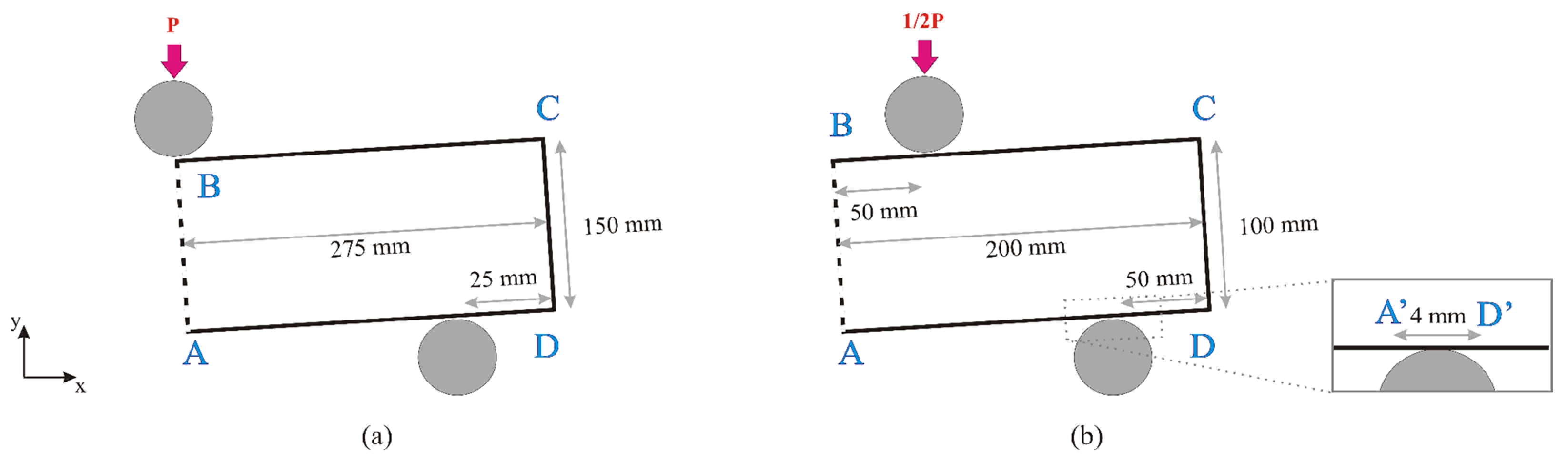
• The constant displacement du^s = 0 and the rotation angle θ^s = 0 is defined for the support (lower) roller. The roller of the test machine (upper) is loaded with the displacement du^t, but the angle θ^t = 0 (see Figure 4).
• The constant displacement du^s = 0 is defined for the support roller; it is loaded with the rotation angle dθ^s. For the roller of the test machine, the displacement is constant du^t = 0, and the angle is zero.
• The support roller has the constant displacement du^s = 0 and the rotation angle θ^s = 0, while the roller of the test machine is loaded with the rotation angle dθ^t, and the displacement is constant du^t = 0.
• The support roller has the constant displacement du^s = 0, but it is loaded with the rotation angle dθ^s, while the roller of the test machine is loaded with the displacement du^t, but θ^t = 0.
• The support roller has a constant displacement du^s = 0, and the rotation angle is zero. The roller of the test machine is loaded with both the displacement du^t and the angle of rotation dθ^t.
• Both rollers are loaded with the angle of rotation, but the displacements of both rollers are constant.

After finding the constants, energy minimization is performed. Knowing the energy (Equation (1)), we can apply the second theorem of Castigliano to determine the forces by Equation (2) and the moment by Equation (3).

$$-F=\frac{\mathsf{\partial }E}{\mathsf{\partial }u},$$

(2)

$$-M=\frac{\mathsf{\partial }E}{\mathsf{\partial }\theta },$$

(3)

where u is the displacement, and θ is the angle, see Figure 4b.

3.2. Analyzed Bridging Law Functions

The bridging law is the main input required by the FE model to characterize both the matrix and the fibers. Parameters such as the effects of moisture ingress or environmental aging, as well as fiber orientation, volume fraction, or surface treatment, are not defined in the FE model, but by the chosen bridging law. Comparing the modeling results with the experiments, bilinear and nonlinear bridging law functions were used for further modeling. Both functions require the following parameters to characterize them: the tensile strength f_t and the fracture energy G_F.

Based on Herrmann and Roux [51], the fracture energy G_F is defined as the area average of the fracture work calculated by Equation (4).

$$G_F=\frac{W}{A_{lig}},$$

(4)

where W represents the work for generating the new surface, and A_lig is the ligament area formed at the front of the initial crack. The fracture work absorbed by the material throughout the fracture process in the bending test can be calculated by Equation (5).

$$W={{\displaystyle \int }}_a^{b}Pdu,$$

(5)

where P represents the external loading, du represents the change in the CMOD (or δ), and a and b are the lower and upper limits of the CMOD (or δ) [52].

3.2.1. Bilinear Bridging Law Function

The expressions for the bilinear bridging law function described by Guinea et al. [35] are the following:

$$\{\begin{array}{c}\sigma =f_t\left(1-w/w_1\right),for 0<w<w_k\\ \sigma ={\sigma }_k\frac{\left(w-w_c\right)}{w_k-w_c},for w_k<w<w_c\\ \sigma =0, for w\ge w_c\end{array},$$

(6)

where σ is stress, w₁ = 1.2 (G_F/f_t) is the horizontal intercept of the steeper segment, and σ_k, w_k are the coordinates of the kink point, given by Equations (7) and (8), respectively.

$$w_k=\frac{w_1\left(w_c-2\left(G_F/f_t\right)\right)}{w_c-w_1}$$

(7)

$${\sigma }_k=\frac{f_t \left(2\left(G_F/f_t\right)-w_1\right)}{w_c-w_1}$$

(8)

The critical opening w_c is obtained from the quadratic equation:

$$w_c{}^2-w_c \frac{6\overline{w}\left(G_F/f_t\right)-2w_1\left(G_F/f_t\right)}{2\left(G_F/f_t\right)-w_1}+\frac{6\overline{w}{w}_1\left(G_F/f_t\right)-4w_1{(G_F/f_t)}^2}{2\left(G_F/f_t\right)-w_1}=0,$$

(9)

where $\overline{\mathrm{w}}$ is the abscissa of the centroid of the bridging law curve calculated by Equation (10).

$$\overline{w}=\alpha G_F/f_t$$

(10)

α is a dimensionless parameter, which, for a bilinear function, is 0.987 according to Petersson [53] or 1.1–1.3 according to Reinhardt et al. [54]. In the analyzed cases, the best agreement with the experiment was given by α = 1.1.

3.2.2. Nonlinear Bridging Law Function

The nonlinear bridging law function developed by Cornelissen et al. [37] is proposed in the following form:

$$\sigma =f_t\left(\left[1+{\left(\frac{c_{1}w}{w_c}\right)}^3\right]\cdot exp\left(\frac{-c_{2}w}{w_c}\right)-\frac{w}{w_c}\left(1+c_1{}^3\right)exp\left(-c_2\right)\right),$$

(11)

where c₁, c₂, and w_c are material constants. For analyzed concrete, the three parameters are considered as c₁ = 2.5, c₂ = 6.93 and the critical opening is obtained by Equation (12).

$$w_c=5.136\frac{G_F}{f_t}$$

(12)

3.3. Surrogate Modeling

The use of surrogate models helps to effectively understand and evaluate the interdependence of model factors (inputs) and responses (output) without full-scale numerical simulations or experiments. In the general case, the goal is to obtain a response function F (as in Equation (13)) that depends on the values of the factors x_i.

F = f(x₁,x₂,…,x₃),

(13)

where x₁, x₂, … x_n are coordinates from the factor space. The response function F in the factor space represents the response surface.

This research examined the first, second, and third-order polynomial approximations. The coefficient of determination R² and Pearson’s χ² test were used to characterize the fit of the surrogate model. In addition, a leave-one-out cross-validation approach was used for surrogate model verification. Leave-one-out cross-validation is a cross-validation method that involves using one observation as validation data, and the remaining data are used to train the model. For example, point i = 1 is selected for validation in the first iteration for a data set with N points, and the remaining (N-1) points are used for model building. For the second iteration, point i = 2 is selected for validation, and the remaining ones are for building the model. The process is repeated N times. A smaller cross-validation value means a higher accuracy of the surrogate model. The cross-validation percentage error is defined in Equation (14) to avoid overestimating the prediction error.

$$Erro{r}_{cv}=\frac{\sqrt{\frac{1}{N}{{\displaystyle \sum }}^{}{(\widehat{y_i}-y_i)}^2}}{\frac{1}{N}{{\displaystyle \sum }}^{}{y}_i}100\%,$$

(14)

where $\widehat{y_i}$ is the approximation, ignoring point i (i = 1, 2, …, N). A surrogate model is assumed to have acceptable accuracy if the cross-validation error is less than 10% for numerical experiments and less than 5% for physical experiments.

4. Numerical Examples

To validate the suitability of the FE modeling approach discussed above for studying the mechanical properties of fiber concrete, modeling was carried out for 3PBT and 4PBT using the same sample batches as in the experiments. Considering that prisms with a single notch are used in the 3PBT experiments, the nodes of the corresponding elements on both sides of the crack patch are also marked as unconnected in the FE model before calculations. The existence of a notch fits well with the model’s assumption that the crack will originate in the middle of the sample in a horizontal direction and propagate vertically upwards. Three notched concrete prism examples without and with BFs under 3PBT and examples of concrete beams with two doses of BFs and three doses of OSA under 4PBT were simulated. A surrogate model describing the maximum load P_max as a function of the tensile strength f_t and the fracture work W was created using the 4PBT modeling results for a concrete specimen with BFs and OSA.

FE models with corresponding dimensions are shown in Figure 5 for both bending tests.

To evaluate the influence of the size of the cell elements on the obtained result, three types of meshes were examined for the concrete sample from Batch C. The calculated maximum force values depending on the maximum size of mesh elements are summarized in

Table 3. Effect of cell size on maximum force.

Case	The Number of Elements in the FE Model	The Number of Nodes	Pmax (kN)
M1	8600	3891	9.79
M2	2456	1025	9.83
M3	749	274	9.98

. Considering the obtained results and the time required for computing, a mesh with 2456 elements was chosen as the optimal case for further calculations. An example of a computational domain mesh can be seen in Figure 6. In addition, the refinement of mesh elements was applied to the crack path AB (see Figure 5) and the contact surfaces of the rollers with the sample (see A’D’ in Figure 6). First-order triangular finite elements are used for simulations. Linear triangular elements have been widely used in engineering problems because of their adaptability to complex models, simple calculations, and acceptable accuracy [55].

The display of the bending test result—P-CMOD or P-δ curve can be divided into three parts, see Figure 7. The first ascending part of the curve corresponds to the linear phase. After the linear part, the matrix failure phase begins, in which cracks start to propagate in the concrete matrix. The load reaches its maximum value. In the third phase, continuing to increase the external load, the fibers begin to work—they are pulled out and/or broken.

An example of the stress distribution in the Batch C sample obtained by the FE model is shown in Figure 8. Figure 8a shows that the solution in the linear phase corresponds to the Euler–Bernoulli beam theory. The upper left corner of the sample shows compression, while the lower left corner shows tension. Places of loading and supporting rollers are also well visible. While in the matrix failure phase, when the crack starts to open, the stress field has changed significantly, see Figure 8b. The tension-dominated area of the crack path has increased considerably.

4.1. Three-Point Bending Tests

The P-CMOD curve obtained in FE modeling and measured in experiments for samples in the three-point bending test can be seen in Figure 9. The reference samples are without basalt fibers (Batch A0); see Figure 9a. In addition, samples with 6.7 kg per 1 m³ (see Figure 9b, Batch A1) and 10.8 kg per 1 m³ (see Figure 9c, Batch A2) doses of composite BFs in the mixture are analyzed. In the figures, the black dotted line represents the mean values of three experiments for Batch A0 and the mean values of six samples for the other groups. Error bars show the standard deviation for 3PBT. The blue line represents the P-CMOD curve obtained by the FE modeling using the bridging law concept.

The average peak load from the three experiments for the case without BFs (see Figure 9a) is 17.4 kN, achieved when the CMOD is 0.033 mm. The FE model with the bilinear bridging law function predicts the maximum load at 17.62 kN. The peak is reached when CMOD is 0.034 mm. When using a nonlinear bridging law function, the maximum load is 17.9 kN, which is reached at 0.036 mm. Comparing the values of the fracture work (from the P-CMOD curves), it can be found that in the case of the bilinear function (W = 2.74 Nm), it is closer to the experimental value (W = 2.30 Nm) than the result of the nonlinear function (W = 3.39 Nm).

The maximum load of the concrete sample with 6.7 kg per 1 m³ of BFs (Batch A1) is 15.8 kN when CMOD = 0.036 mm. The comparison of the experimental and modeling results of Batch A1 shows that the bilinear bridging law function better describes the trends of the linear part of the P-CMOD curve and cracking phase in the concrete matrix but incorrectly predicts the fiber failure phase. The nonlinear function overestimates the peak load (P_max = 17.76 kN at 0.054 mm). However, it best describes the fiber failure phase.

Adding 10.8 kg of BFs per 1 m³ to the mixture (Batch A2), tested on six samples, reduces the peak load value to 14.1 kN. CMOD value is 0.033 mm. It can be seen in Figure 9c that the FE model predicts a significantly higher load peak value (P_max = 17.32 kN at CMOD = 0.074 mm) and a slower sample rupture than was obtained in the experiment. The addition of longer composite BFs causes considerable damage to the specimen volume in the bending test. Therefore, the assumption used in the FE modeling about damage formation only around the fiber surface is not true in this case. For this reason, a faster decrease in the P-CMOD curve is observed in the experiment after the maximum loading than predicted by the FE model. Modeling such cases (with longer fiber pull-outs) should also consider micromechanics models.

The results of the FE model of the 3PBT show that for the bending test modeling of BF concrete samples, a more accurate P-CMOD curve is obtained using the nonlinear bridging law function, and for plain concrete (0.0% BF)—a bilinear function.

4.2. Four-Point Bending Tests

The comparison of the experimental and FE model results of the 4PBT shows that the bilinear bridging law function best fits the experimental results of Batch B (the dose of BFs is 15.7 kg per 1 m³). It follows from

Table 4. Comparison of experimental and FE model (with bilinear bridging law) results for Batch B samples.

OSA (%)	FE Modeling		Experiments
	Pmax (kN)	δPmax (mm)	Pmax (kN) (stdev)	δPmax (mm) (stdev)
10	10.72	0.094	9.93 (0.16)	0.05 (0.004)
15	10.23	0.104	10.45 (0.33)	0.05 (0.006)
30	9.75	0.10	9.97 (0.42)	0.05 (0.007)

that the maximum load obtained with the FE model is close to the experimentally measured values. The standard deviation stdev of four experiments is shown in brackets. The midspan deflection δ_Pmax, at which these maximum values are reached, is 0.05 mm in the experiments, regardless of the amount of added OSA, but in the FE model, the deflection is larger, i.e., 0.09–0.1 mm. However, comparing the P-δ curve obtained in the experiments with the results of the FE model, it can be concluded that the model predicts the general trends of crack propagation.

In the case of Batch C samples (the dose of BFs is 23.7 kg per 1 m³), the experimental P-δ curve is most accurately represented by the FE model with a nonlinear bridging law function. The obtained results are summarized in

Table 5. Comparison of experimental and FE model (with nonlinear bridging law) results for Batch C samples.

OSA (%)	FE Modeling		Experiments
	Pmax (kN)	δPmax (mm)	Pmax (kN) (stdev)	δPmax (mm) (stdev)
10	7.82	0.104	7.44 (0.64)	0.14 (0.04)
20	7.73	0.112	7.90 (0.67)	0.16 (0.05)
30	9.91	0.104	9.64 (0.59)	0.15 (0.05)

. It can be seen that the FE model can predict the maximum loads and the corresponding midspan deflection values of the samples of this group according to the experimentally measured values under the 4PBT.

Summarizing the obtained modeling results of 4PBTs for samples with BFs and OSA, the bilinear function is the most suitable bridging law for samples with a smaller number of added fibers. On the other hand, if the BF dose is 23.7 kg per 1 m³, a more accurate P-δ curve can be obtained with a nonlinear bridging law function. At higher BF doses, the model fits well with the experimental data for the peak loading P_max and the corresponding midspan deflection δ_Pmax value. Although preliminary results show that the nonlinear function gives a more accurate bending test result in mixtures with higher fiber content, more research is needed to confirm this conclusion.

The results show that adding OSA to the mixture of Batch B samples does not significantly affect the maximum load values. On the other hand, the load peak value for Batch C samples increases with the addition of OSA; i.e., with 10% OSA, the maximum is 7.44 kN, while with 30% OSA, it increases to 9.64 kN.

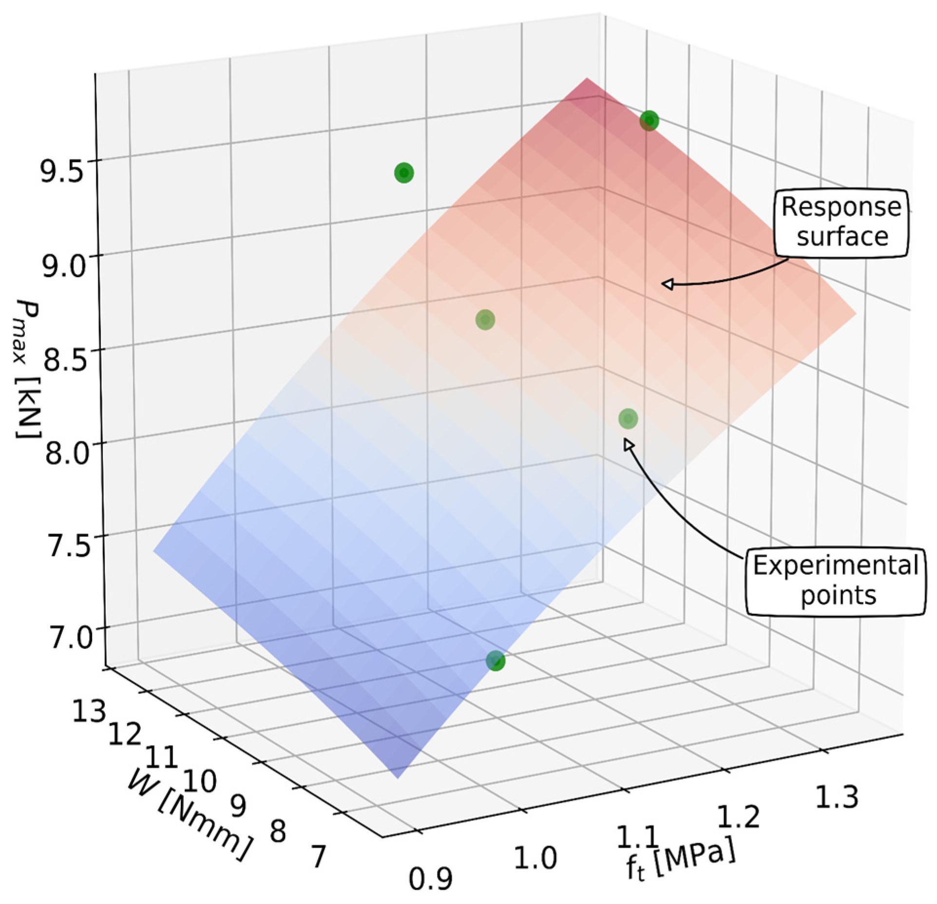
4.3. Surrogate Model to Predict Maximum Load in 4PBT

The 13-point orthogonal design of experiments [56] is chosen to create a surrogate model for predicting maximum loads depending on two factors (tensile strength f_t and fracture work W) for the 4PBT. In the design of experiments, orthogonality is essential because it leads to the best models and reduces the variance of the regression coefficients. The building set uses BF concrete supplemented with OSA, as in Batch C. The design of the experiments is shown in Figure 10. Based on the experiments, the following factor space was chosen: f_t = [0.98; 1.31] (MPa) and W = [6.5; 12.7] (Nm). The validation set consists of five experimental data points of Batch C.

The cross-validation error and the coefficient of determination of the analyzed three polynomial approximations are summarized in

Table 6. Cross-validation errors and R² for polynomial approximation.

Polynomial	Cross-Validation Error	R2
1st order	10.65%	0.993
2nd order	1.17%	0.999
3rd order	0.47%	0.999

. The coefficient of determination R² for all cases shows that the surrogate model agrees with the FE model. On the other hand, from the calculated cross-validation error, it can be concluded that the first-order polynomial approximation provides the worst fitting to the FE model results, and the third-order polynomial approximation provides the best. The cross-validation error of the surrogate model using a third-order polynomial for approximation is less than 0.5%. In all cases, Pearson’s χ² criterion is met.

The resulting equation describing the peak load P_max as a function of f_t and W is shown in Equation (15).

P_max(t_f, W) = −1.9534401 + 14.166294f_t + 0.060235196W − 7.5494805f_t² + 0.25515142f_tW − 0.012196241W² + 1.6287772f_t³ − 0.037482758f_t²W − 0.0042167212f_tW² + 0.00041631893W³.

(15)

The response surface obtained by the third-order polynomial approximation (Equation (15)) is shown in Figure 11. The experimental points of the 4PBT are shown with green dots.

It can be seen from Figure 11 that in certain areas of the design space, the P_max values predicted by the surrogate model are lower than the experimentally measured ones. When calculated, the coefficient of determination is 0.764. To increase the accuracy of the surrogate model, the methodology for finding the tensile strength f_t should be improved.

5. Conclusions

The study focused on the correlation between the experimental and numerical simulation of a new type of concrete containing various doses of oil shale ash and two types of composite basalt fibers. In total, nine concrete mixes were designed and tested in a fresh and hardened state. Batch A contained BFs with a length of 43 mm and was characterized by E-modulus between 28.7 and 29.8 GPa and residual flexural tensile strength test with loads at the limit of proportionality between 14.1 and 17.4 kN. Batches B and C were designed with various doses of BFs with a length of 25 mm and a replacement of 10, 15, 20, and 30% of cement by oil shale ash. The maximum load of four-point bending tests ranged between 7.44 and 10.45 kN.

Experimental results from three-point and four-point bending tests were compared to numerical simulations. In developing the finite element model, an approximation of small angles and deformations was adopted, corresponding to the experimentally observed behavior. The modeling considered changes in the contact surfaces between the concrete prism and the rollers during the bending test.

For studying the properties of new materials (with several parameters), numerical modeling provides obvious advantages compared to experiments—preparing samples and performing mechanical tests take weeks (tests are typically performed after 28 days) or longer (after 56 or 90 days), while obtaining modeling results takes a few hours.

The most appropriate bridging law is a bilinear function for samples with or without a small dose of shorter basalt fibers (24 mm). On the other hand, if the BF dose is higher, a more accurate P-δ curve can be obtained with a nonlinear bridging law function. However, it should be noted that these are preliminary results that need to be verified using an extensive set of experimental data.

Considering that adding longer composite BFs (43 mm) causes significant damage in the sample volume during the bending test, the applied FE modeling methodology can only provide a general assessment of the bending test parameters.

A surrogate model for predicting the maximum load as a function of tensile strength and fracture work was created. From the calculated cross-validation error, it can be concluded that the third-order polynomial approximation best fits the FE modeling results. The cross-validation error was less than 0.5%.

In further research, the authors would like to focus firstly on collecting more experimental data for reliable calibration of the models and applying a probabilistic description of cracking with the involvement of 3D models with finite displacements for bridging-law identification while leaving the 2D approach still valid for structural optimization. The second priority is the description of crack-related volumetric degradation of the material.

References

1. UN Environment; Scrivener, K.L.; John, V.M.; Gartner, E.M. Eco-efficient cements: Potential economically viable solutions for a low-CO2 cement-based materials industry. Cem. Concr. Res. 2018, 114, 2–26. [Google Scholar] [CrossRef]
2. Low-Carbon Concrete and Construction: A Review of Green Public Procurement Programmes. Available online: https://www.iea.org/reports/cement (accessed on 5 May 2023).
3. Uibu, M.; Somelar, P.; Raado, L.-M.; Irha, N.; Hain, T.; Koroljova, A.; Kuusik, R. Oil shale ash based backfilling concrete—Strength development, mineral transformations and leachability. Constr. Build. Mater. 2016, 102, 620–630. [Google Scholar] [CrossRef]
4. Hemalatha, T.; Ramaswamy, A. A review on fly ash characteristics—Towards promoting high volume utilization in developing sustainable concrete. J. Clean. Prod. 2017, 147, 546–559. [Google Scholar] [CrossRef]
5. Irha, N.; Uibu, M.; Jefimova, J.; Raado, L.-M.; Hain, T.; Kuusik, R. Leaching behaviour of Estonian oil shale ash-based construction mortars. Oil Shale 2014, 31, 394–411. [Google Scholar] [CrossRef] [Green Version]
6. Othman, H.; Sabrah, T.; Marzouk, H. Conceptual design of ultra-high performance fiber reinforced concrete nuclear waste container. Nucl. Eng. Technol. 2018, 51, 588–599. [Google Scholar] [CrossRef]
7. Carvalho, M.R.; Barros, J.; Zhang, Y.; Dias-Da-Costa, D. A computational model for simulation of steel fibre reinforced concrete with explicit fibres and cracks. Comput. Methods Appl. Mech. Eng. 2020, 363, 112879. [Google Scholar] [CrossRef]
8. Dhand, V.; Mittal, G.; Rhee, Y.K.; Park, S.J.; Hui, D. A short review on basalt fibre reinforced polymer composites. Composites Part B Eng. 2015, 73, 166–180. [Google Scholar] [CrossRef]
9. Alnahhal, W.; Aljidda, O. Flexural behavior of basalt fiber reinforced concrete beams with recycled concrete coarse aggregates. Constr. Build. Mater. 2018, 169, 165–178. [Google Scholar] [CrossRef]
10. Novakova, I.; Thorhallsson, E.R.; Wallevik, O.H. Influence of environmentally friendly basalt fibres on early-age strength development. In Proceedings of the Fib Symposium Kraków, Krakow, Poland, 27–29 May 2019; pp. 266–273. [Google Scholar]
11. Bheel, N. Basalt fibre-reinforced concrete: Review of fresh and mechanical properties. J. Build. Pathol. Rehabilitation 2021, 6, 12. [Google Scholar] [CrossRef]
12. Monaldo, E.; Nerilli, F.; Vairo, G. Basalt-based fiber-reinforced materials and structural applications in civil engineering. Compos. Struct. 2019, 214, 246–263. [Google Scholar] [CrossRef]
13. George, E.H.; Bhuvaneshwari, B.; Palani, G.S.; Sakaria, P.E.; Iyer, N.R. Effect of Basalt Fibre on Mechanical Properties of Concrete Containing Fly Ash and Metakaolin. Int. J. Innov. Res. Sci. Eng. Technol. 2014, 3, 444–451. [Google Scholar]
14. Jia, Z.-M.; Zhou, X.-P. Field-enriched finite element method for simulating complex cracks in brittle solids. Eng. Fract. Mech. 2022, 268, 108504. [Google Scholar] [CrossRef]
15. Zienkiewicz, O.C.; Taylor, R.L.; Zhu, J.Z. The Finite Element Method: Its Basis and Fundamentals, 7th ed.; Butterworth Heinemann: Oxford, UK, 2013. [Google Scholar] [CrossRef]
16. Quek, S.S.; Liu, G.R. The Finite Element Method: A Practical Course; Butterworth-Heinemann: Oxford, UK, 2003. [Google Scholar]
17. Khormani, M.; Jaari, V.R.K.; Aghayan, I.; Ghaderi, S.H.; Ahmadyfard, A. Compressive strength determination of concrete specimens using X-ray computed tomography and finite element method. Constr. Build. Mater. 2020, 256, 119427. [Google Scholar] [CrossRef]
18. Le, L.A.; Nguyen, G.D.; Bui, H.H.; Sheikh, A.H.; Kotousov, A. Incorporation of micro-cracking and fibre bridging mechanisms in constitutive modelling of fibre reinforced concrete. J. Mech. Phys. Solids 2019, 133, 103732. [Google Scholar] [CrossRef]
19. Gu, Y.; Zhang, C. Novel special crack-tip elements for interface crack analysis by an efficient boundary element method. Eng. Fract. Mech. 2020, 239, 107302. [Google Scholar] [CrossRef]
20. Li, C.; Niu, Z.; Hu, Z.; Hu, B.; Cheng, C. Effectiveness of the stress solutions in notch/crack tip regions by using extended boundary element method. Eng. Anal. Bound. Elements 2019, 108, 1–13. [Google Scholar] [CrossRef]
21. Jiang, S.; Gu, Y.; Fan, C.-M.; Qu, W. Fracture mechanics analysis of bimaterial interface cracks using the generalized finite difference method. Theor. Appl. Fract. Mech. 2021, 113, 102942. [Google Scholar] [CrossRef]
22. Yan, C.; Zheng, Y.; Wang, G. A 2D adaptive finite-discrete element method for simulating fracture and fragmentation in geomaterials. Int. J. Rock Mech. Min. Sci. 2023, 169, 105439. [Google Scholar] [CrossRef]
23. Ren, H.; Song, S.; Ning, J. Damage evolution of concrete under tensile load using discrete element modeling. Theor. Appl. Fract. Mech. 2022, 122, 103622. [Google Scholar] [CrossRef]
24. Planas, J.; Elices, M.; Guinea, G.; Gómez, F.; Cendón, D.; Arbilla, I. Generalizations and specializations of cohesive crack models. Eng. Fract. Mech. 2003, 70, 1759–1776. [Google Scholar] [CrossRef]
25. Elices, M.; Rocco, C.; Roselló, C. Cohesive crack modelling of a simple concrete: Experimental and numerical results. Eng. Fract. Mech. 2009, 76, 1398–1410. [Google Scholar] [CrossRef]
26. Bažant, Z.P.; Planas, J. Fracture and Size Effect in Concrete and Other Quasibrittle Materials; Taylor & Francis: New York, NY, USA, 1998; 640p. [Google Scholar]
27. Ambati, M.; Gerasimov, T.; De Lorenzis, L. A review on phase-field models of brittle fracture and a new fast hybrid formulation. Comput. Mech. 2014, 55, 383–405. [Google Scholar] [CrossRef]
28. Lammen, H.; Conti, S.; Mosler, J. A finite deformation phase field model suitable for cohesive fracture. J. Mech. Phys. Solids 2023, 178, 105349. [Google Scholar] [CrossRef]
29. Lateef, H.A.; Laftah, R.M.; Jasim, N.A. Investigation of crack propagation in plain concrete using Phase-field model. Mater. Today Proc. 2022, 57, 375–382. [Google Scholar] [CrossRef]
30. Feng, D.-C.; Wu, J.-Y. Phase-field regularized cohesive zone model (CZM) and size effect of concrete. Eng. Fract. Mech. 2018, 197, 66–79. [Google Scholar] [CrossRef]
31. Li, H.; Huang, Y.; Yang, Z.; Yu, K.; Li, Q. 3D meso-scale fracture modelling of concrete with random aggregates using a phase-field regularized cohesive zone model. Int. J. Solids Struct. 2022, 256, 111960. [Google Scholar] [CrossRef]
32. Niu, Y.; Wei, J.; Jiao, C. Multi-scale fiber bridging constitutive law based on meso-mechanics of ultra high-performance concrete under cyclic loading. Constr. Build. Mater. 2022, 354, 129065. [Google Scholar] [CrossRef]
33. Qiu, J.; Yang, E.-H. A micromechanics-based fatigue dependent fiber-bridging constitutive model. Cem. Concr. Res. 2016, 90, 117–126. [Google Scholar] [CrossRef]
34. Hillerborg, A.; Modéer, M.; Petersson, P.-E. Analysis of crack formation and crack growth in concrete by means of fracture mechanics and finite elements. Cem. Concr. Res. 1976, 6, 773–781. [Google Scholar] [CrossRef]
35. Guinea, G.V.; Planas, J.; Elices, M. A general bilinear fit for the softening curve of concrete. Mater. Struct. 1994, 27, 99–105. [Google Scholar] [CrossRef]
36. Fathy, A.M.; Sanz, B.; Sancho, J.M.; Planas, J. Determination of the bilinear stress-crack opening curve for normal- and high-strength concrete. Fatigue Fract. Eng. Mater. Struct. 2008, 31, 539–548. [Google Scholar] [CrossRef]
37. Cornelissen, H.A.W.; Hordijk, D.; Reinhardt, H. Experimental determination of crack softening characteristics of normalweight and lightweight concrete. HERON 1986, 31, 45–56. [Google Scholar]
38. Karihaloo, B.L. Fracture Mechanics and Structural Concrete, Concrete Design and Construction Series; Longman Scientific & Technical: London, UK, 1995. [Google Scholar]
39. Lukasenoks, A.; Macanovskis, A.; Krasņikovs, A.; Lapsa, V. Composite fiber pull-out in concretes with various strengths. In Proceedings of the 15th International Sci-entific Conference on Engineering for Rural Development, Jelgava, Latvia, 25 May 2016; pp. 1417–1423. [Google Scholar]
40. Macanovskis, A.; Lukasenoks, A.; Krasnikovs, A.; Stonys, R.; Lusis, V. Composite fibers in concretes with various strengths. ACI Mater. J. 2018, 115, 647–652. [Google Scholar] [CrossRef]
41. Lapsa, V.; Krasnikovs, A. Composite Material Fiber and its Production Process. Latvian Patent LV15339, 20 March 2021. [Google Scholar]
42. MiniBars. Available online: https://reforcetech.com/technology/minibars/ (accessed on 11 July 2023).
43. Ramesh, B.; Eswari, S. Mechanical behaviour of basalt fibre reinforced concrete: An experimental study. Mater. Today Proc. 2021, 43, 2317–2322. [Google Scholar] [CrossRef]
44. Chen, X.-F.; Kou, S.-C.; Xing, F. Mechanical and durable properties of chopped basalt fiber reinforced recycled aggregate concrete and the mathematical modeling. Constr. Build. Mater. 2021, 298, 123901. [Google Scholar] [CrossRef]
45. EN 14651:2005+A1:2007; Test Method for Metallic Fibre Concrete-Measuring the Flexural Tensile Strength (Limit of Proportionality (LOP), Residual). Available online: https://www.en-standard.eu/bs-en-14651-2005-a1-2007-test-method-for-metallic-fibre-concrete-measuring-the-flexural-tensile-strength-limit-of-proportionality-lop-residual/ (accessed on 5 May 2023).
46. Turbobuild Integral. Available online: https://www.deutsche-basalt-faser.de/en/products/turbobuild-integral/ (accessed on 5 May 2023).
47. EN 12390-5:2009; Testing Hardened Concrete. Flexural Strength of Test Specimens. Available online: https://www.en-standard.eu/bs-en-12390-5-2019-testing-hardened-concrete-flexural-strength-of-test-specimens/ (accessed on 5 May 2023).
48. Lindhagen, J.; Jekabsons, N.; Berglund, L. Application of bridging-law concepts to short-fibre composites 4. FEM analysis of notched tensile specimens. Compos. Sci. Technol. 2000, 60, 2895–2901. [Google Scholar] [CrossRef]
49. Li, H.; Yang, Z.-J.; Li, B.-B.; Wu, J.-Y. A phase-field regularized cohesive zone model for quasi-brittle materials with spatially varying fracture properties. Eng. Fract. Mech. 2021, 256, 107977. [Google Scholar] [CrossRef]
50. Mujika, F.; Arrese, A.; Adarraga, I.; Oses, U. New correction terms concerning three-point and four-point bending tests. Polym. Test. 2016, 55, 25–37. [Google Scholar] [CrossRef]
51. Herrmann, H.J.; Roux, S. Statistical Models for the Fracture of Disordered Media; Elsevier: Amsterdam, The Netherlands, 2014. [Google Scholar]
52. Zhang, C.; Shi, F.; Cao, P.; Liu, K. The fracture toughness analysis on the basalt fiber reinforced asphalt concrete with prenotched three-point bending beam test. Case Stud. Constr. Mater. 2022, 16, e01079. [Google Scholar] [CrossRef]
53. Petersson, P.E. Crack Growth and Development of Fracture Zone in Plain Concrete and Similar Materials. TVBM-1006 ed. Ph.D. Thesis, Division of Building Materials, Lund Institute of Technology, Lund, Sweden, 1981. [Google Scholar]
54. Reinhardt, H.W.; Cornelissen, H.A.W.; Hordijk, D.A. Tensile tests and failure analysis of concrete. J. Struct. Eng. ASCE 1986, 112, 2462–2477. [Google Scholar] [CrossRef]
55. Cui, X.; Liu, G.; Li, Z. A high-order edge-based smoothed finite element (ES-FEM) method with four-node triangular element for solid mechanics problems. Eng. Anal. Bound. Elements 2023, 151, 490–502. [Google Scholar] [CrossRef]
56. Auzins, J. High order orthogonal designs of experiments for metamodeling, identification and optimization of mechanical systems. In Proceedings of the 11th World Congress on Computational Mechanics, 5th European Conference on Computational Mechanics, and 6th European Conference on Computational Fluid Dynamics, Barcelona, Spain, 20–25 July 2014; pp. 3190–3201. [Google Scholar]
57. Jekabsons, J. Mechanics of Composites with Fiber Bundle Meso-Structure. Ph.D. Thesis, Luleå University of Technology, Luleå, Sweden, 2002. [Google Scholar]
58. Shewchuk, J.R. Triangle: Engineering a 2D Quality Mesh Generator and Delaunay Triangulator; Carnegie Mellon University: Pittsburgh, PA, USA, 2005. [Google Scholar]
Figure 1. The flowchart of the study.
Buildings 13 01868 g001
Figure 2. Basalt composite fiber MiniBar (a) compact, (b) broken.
Buildings 13 01868 g002
Figure 3. Results of CMOD testing. Average of 6 samples for mix A1 and A2, and 3 samples for A0.
Buildings 13 01868 g003
Figure 4. Sketch of FE model with (a) midspan deflection δ and crack mouth opening displacement CMOD and (b) introduced generalized coordinates.
Buildings 13 01868 g004
Figure 5. Geometry and dimensions of the FE model for the (a) 3PBT and (b) 4PBT.
Buildings 13 01868 g005
Figure 6. An example of a computational domain mesh. On the x and y axis is the length in millimeters.
Buildings 13 01868 g006
Figure 7. FE modeling result for 4PBT: P-delta curve and corresponding phases in it.
Buildings 13 01868 g007
Figure 8. An example of the stress field distribution in the computational domain at different failure phases: (a) linear phase; (b) matrix failure phase. Four-point bending test. On the axes are the sample dimensions in mm. The color scale corresponds to stress σ in MPa.
Buildings 13 01868 g008aBuildings 13 01868 g008b
Figure 9. Comparison of FE model and experiments for the 3PBT: (a) Batch A0 (without BFs); (b) Batch A1; (c) Batch A2.
Buildings 13 01868 g009aBuildings 13 01868 g009b
Figure 10. Two-factor 13-point orthogonal design of experiments.
Buildings 13 01868 g010
Figure 11. The response surface using the third-order polynomial approximation and experimental points.
Buildings 13 01868 g011